Abstract
The combination of lidar and digital photography provides a new technology for creating a high-resolution 3D digital outcrop model. The digital outcrop model can accurately and conveniently depict the surface 3D properties of an outcrop profile, making up for the shortcomings of traditional outcrop research techniques. However, the advent of digital outcrop poses additional challenges to the 3D spatial analysis of virtual outcrop models, particularly in the interpretation of geological characteristics. In this study, the detailed workflow of automated interpretation of geological characteristics of fractures and cavities on a 3D digital outcrop texture model is described. Firstly, advanced automatic image analysis technology is used to detect the 2D contour of the fractures and cavities in the picture. Then, to obtain an accurate representation of the 3D structure of the fractures and cavities on the digital outcrop model, a projection method for converting 2D coordinates to 3D space based on geometric transformations such as affine transformation and linear interpolation is proposed. Quantitative data on the size, shape, and distribution of geological features are calculated using this information. Finally, a novel and comprehensive automated 3D quantitative characterization technique for fractures and cavities on the 3D digital outcrop texture model is developed. The proposed technology has been applied to the 3D mapping and quantitative characterization of fractures and cavities on the outcrop profile for the Dengying Formation (second member), providing a foundation for profile reservoir appraisal in the research region. Furthermore, this approach may be extended to the 3D characterization and analysis of any point, line, and surface objects derived from outcrop photos, hence increasing the application value of the 3D digital outcrop model.
1. Introduction
Field outcrop is an essential research object in geological work and plays a crucial part in the process of oil and gas geological exploration and development [1,2,3]. Early geologists used photos to depict outcrops by hand drawing and physically measured outcrops using conventional equipment such as a geological compass and ruler. This traditional approach of outcrop study has two obvious disadvantages: (1) operation: based on traditional methods, field mapping in high slopes or unstable areas (desert, arctic, etc.) is very time-consuming and dangerous [4,5]; (2) application: traditional methods represent a much more varied approach and analysis (e.g., measurements, stereograms, and cross-sections are used when the geometry is important). It is also important that sampling is the main advantage of in situ analysis. However, traditional methods for interpreting geological features only use 2D flat photographs, which leads to a lot of inaccuracies [6,7]. In recent years, researchers need more accurate, efficient, and intelligent approaches to analyze the morphological properties of outcrops [8,9,10,11]. Therefore, traditional outcrop research methodologies are unable to suit outcrop research’s application demands at this stage. The development of the 3D digital outcrop model (DOM) provides a feasible solution. Geologists may now produce a high-precision and actual 3D DOM, as well as digitally display and research the DOM on a computer [12,13,14,15,16]. The DOM plays an important role in many studies, including lithologic classification of outcrop section, sequence stratigraphic division, fine interpretation of structural faults, construction of reservoir geological knowledge base, reservoir modeling, etc. [12,13,14,15,16,17,18].
Geologists are frequently interested in multiscale geological features of the outcrop surface in the process of interpreting digital outcrops, such as fractures, bedding, cavities, etc. [19,20,21,22,23,24]. These geological features will be converted into the geologically significant point, line, and surface vector objects. Further analysis of multiple geological features will be carried out based on vector objects. There are three different types of digital outcrop interpretation methods: (1) manual interpretation: researchers manually draw the target object on the digital outcrop surface; (2) automatic interpretation: researchers use computer programs to extract relevant geological features automatically; (3) semiautomatic interpretation: researchers used the method of integrating manual and automatic interpretation. The resolution of manual interpretation based on photographs might be millimeters and centimeters. However, automatic interpretation is frequently more feasible due to the high effort and low efficiency of manual interpretation [25,26]. According to the survey, automatic interpretation is separated into two categories, direct and indirect. In indirect methods, the target geological features are firstly detected based on the outcrop 2D pictures and then translated to the 3D digital outcrop surface [25,27,28]. In direct methods, the target geological features are extracted directly from the 3D data of the outcrop, such as point cloud and triangular mesh [5,7,29].
Machine recognition technology is showing considerable benefits in picture feature extraction at the moment, thanks to the rapid development of artificial intelligence. A vast number of researchers use machine learning to detect relevant characteristics in high-resolution photos, then transfer the data to the outcrop digital elevation model (DEM) for analysis and application [24,25,27,30,31]. In the field of 3D GIS, the properties of the DEM have been discussed [32,33,34]. The DEM can only cope with information on the plane’s X-axis and Y-axis, but not the vertical Z-axis. The precision of the DEM is limited since it projects z-values onto a 2D plane and cannot represent several z-values at the same (x, y) point [32,35,36]. Lidar technology has advanced considerably in recent decades. It can now be used to measure 3D point cloud data from the air and on the ground [37]. The outcrop high-precision mesh model may be generated by triangulating the laser-scanned point cloud. Then, with the mesh model matched with the high-resolution picture, the 3D digital outcrop texture realistic model can be obtained. Nowadays, many geological researchers prefer the 3D digital outcrop texture model developed using lidar scanning because it has greater accuracy and can fulfill object modeling with high complexity [23,38,39,40]. However, the interpretation of the high-precision 3D digital outcrop texture model created by lidar scanning is mostly manual or semiautomatic [41,42,43]. Therefore, there are no complete automatic interpretation and characterization methods or tools for the geological features of the DOM surface (e.g., fractures and cavities).
In this study, an automatic 3D quantitative characterization scheme of fractures and cavities based on lidar is proposed. The proposed scheme is applied to quantitatively characterize and analyze the fractures and cavities in the digital outcrop profile of the Dengying Formation (second member) in Xianfeng, Ebian. Specific contributions are as follows: (1) a high-precision digital outcrop texture model in the study area is established; (2) two types of geology features, fractures and cavities, in outcrop profiles are automatically extracted and characterized; (3) to establish the transformation relationship between 2D texture coordinates of geological features and 3D model coordinates, a 2D and 3D coordinate transformation method based on geometric transformations is proposed; (4) the 3D statistics and analysis of the geological features of fractures and cavities are carried out using the 3D outcrop model.
2. Geological Setting
Sichuan Basin is a typical superimposed basin and is one of the largest petroliferous basins in China. Sichuan Basin consists of six tectonic units, including North Sichuan low-level fold belt, South Sichuan low-steep fold belt, southwest Sichuan low-steep fold belt, West Sichuan depression belt, East Sichuan high-steep fold belt, and central Sichuan flat gentle fold belt [44]. In Sichuan Basin, the majority of carbonate reservoirs developed with dissolved pore and fracture are of great burial depth. In these reservoirs, the fracture opening is low, and the dissolved pore is mainly connected through a fine throat. Dissolution caused the cavity to develop during differentiation. The influence of tectonism and dissolution causes fractures to occur [45,46,47]. The study area is located in the Xianfeng area of Ebian in the southwest of Sichuan Basin (Figure 1a). The selected profile is located in Xianfeng village, Ebian Yi Autonomous County, southwest edge of Sichuan Basin (called Xianfeng profile). Xianfeng profile is a profile from Sinian to Cambrian strata completely exposed in the Sichuan Basin. It is around 45 m long and 10 m tall. The strata are continuous, and the horizon line is clearly defined. Following a review of relevant geological data and surveys, it was discovered that the stratum of the Dengying Formation of the Upper Sinian system in the Xianfeng profile is relatively complete, with little weathering and no vegetation coverage, providing a solid geological foundation for future research. Predecessors divided Dengying Formation into four sections based on lithology combination and electrical characteristics of logging [48,49,50]. The thickness of the first section of Dengying Formation is 20–70 m. The lithology is mainly micrite-powder crystal dolomite and there are a small number of bacteria and algae. The thickness of the second section of Dengying Formation is 440–520 m. Most lithology is argillaceous dolomite. The lower part is an algae rich-section, and the upper part is an algae-poor section. The thickness of the third section of Dengying Formation is 50–100 m. Mudstone and sandstone are the main lithologies. The thickness of the fourth section of Dengying Formation is 260–350 m. Doloarenite, alginate, and stromatolite dolomite are the main lithologies. The strata from Section 1 to Section 4 of Dengying Formation in the Xianfeng profile are generally exposed. The outcrop interpretation area is located in the middle of the second section of the Dengying Formation. It is not only the microbial dolomite development section but also the main reservoir development section [50,51,52]. This section of the outcrop may be separated into four tiny strata based on field geological survey and imaging characteristics (numbers 1, 2, 3, and 4). The sedimentary facies of layers 1, 3, and 4 is algae clastic beach, and the lithology is thick-bedded algal clot dolomite. The sedimentary facies of layer 2 is muddy-dolomitic flat microfacies, and the lithology is unequal thickness interbedding of medium-thick layered algal clot dolomite and gray-black algal clot dolomite (Figure 1b). The thickness of each layer is as follows: layer 1 (2 m), layer 2 (3.2 m), layer 3 (1.4 m), and layer 4 (1.8 m).
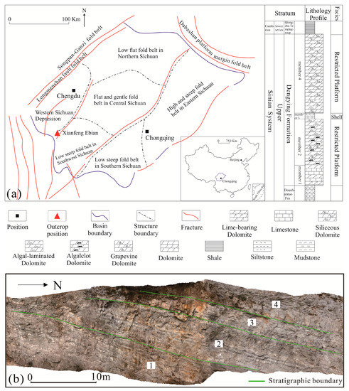
Figure 1.
Geological setting. (a) Location map and stratigraphic histogram of the study area. (b) Outcrop profile for the Dengying Formation (second member).
3. Materials and Methods
3.1. Creation of Digital Outcrop Models
All effort begins with the creation of a DOM. The use of a high-precision DOM has been crucial for both (1) identifying geological characteristics and (2) extracting accurate dimensions for 3D quantitative characterization. Three-dimensional laser scanning is a measuring technique that relies on laser ranging and is commonly used in geoscience. The 3D coordinates, reflectivity, and texture of dense spots on the surface of the scanned object may be accurately captured using 3D laser scanning, and the resolution of 3D laser scanning can reach millimeters [38,40]. In this study, the 3D laser point cloud data of the whole research region was obtained using the Austrian Riegl-vz400 laser scanner. The high-precision texture image of the outcrop was obtained using the Pentax 645D high-resolution digital camera. We begin by constructing the triangulated irregular network (TIN) from the point cloud data, then we paste the high-precision texture picture on the surface of the triangulated irregular network (TIN), and ultimately we obtain the 3D DOM with genuine texture. The workflow used for the creation of the DOM involves the following steps (Figure 2a). (1) Data preparation, including laser scanner, camera, topographic map, aerial photo data, etc. (2) Data acquisition, collecting high-resolution outcrop picture data (Figure 2b) and 3D point cloud data (Figure 2c). (3) Data processing, entering the whole data from the laser point cloud into Geomagic (software for model building), and outputting the result in PLY format. Then, we open the PLY format data into the Polywork (software for model refining), fill the holes in the 3D model, and output the optimized model in .pol format (Figure 2d). Finally, the camera images and the optimized model are precisely co-registered by using Model Painter (software for texture mapping) (Figure 2e). (4) Model output: after verification, the 3D DOM is converted to OBJ standard format and output.
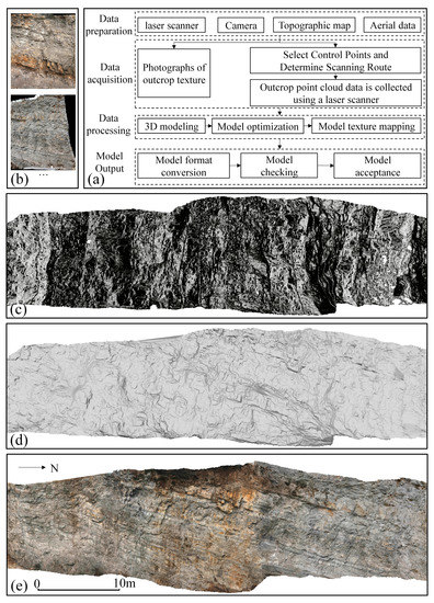
Figure 2.
Workflow of DOM creation based on lidar. (a) The primary workflow. (b) Outcrop high-definition picture data captured using a digital camera. (c) 3D point cloud of outcrop collected by lidar. (d) 3D digital outcrop mesh model. (e) 3D digital outcrop texture model.
3.2. Feature Detection
The total profile may be visually observed when the DOM is generated. Yet, at this moment, the DOM model can only display the 3D geometry of the outcrop profile, and it lacks the ability to extract and analyze essential geological thematic data. As a result, we want to merge the DOM with geological data from the outcrop surface, such as fractures and cavities. In a previous stage, the author’s team proposed a novel multiscale regional convolution neural network detection approach [24] for the detection of carbonate rock cavities features in 2D outcrop images based on the deep learning mask R-CNN model. Mask-RCNN is a deep learning model that can reach pixel-level instance segmentation. Its detection process mainly includes three steps. First, features are extracted through a convolutional neural network, and we used Resnet101 as the backbone feature extraction network. Second, the proposed regions are extracted through the region proposal net-work (RPN). Finally, the feature images are input into fully connected layer and the fully convolutional networks, respectively, to obtain the results of regression, classification, and image segmentation. This approach has a greater detection accuracy than the classic image recognition method, and it may partially replace manual detection The method of reference [27] is utilized in this research to detect fractures in a digital outcrop texture picture by using high-resolution digital outcrop photographs. This method uses phase consistency to detect fracture characteristics [53]. The main advantage of this method over other widely used methods is that phase congruency results are largely invariant to image contrast changes. We used the phase congruency algorithm to detect both visually faint and strong edges from images. The phase congruency output is then processed to remove noise and then thresholded to delineate edge pixels from others. At this time, fractures often appear in the form of discontinuous line segments on the original image. Next, the broken line segments need to be connected automatically or manually. The detected fractures are output as vector graphics and recorded in pixel coordinates. Automatic detection accuracy is determined by the algorithm and the picture resolution. We may complement and change the automated interpretation results in the form of man–machine interaction to reduce the mistake of automatic interpretation in the interpretation process.
3.3. Converting 2D Vector Graphics to 3D Space
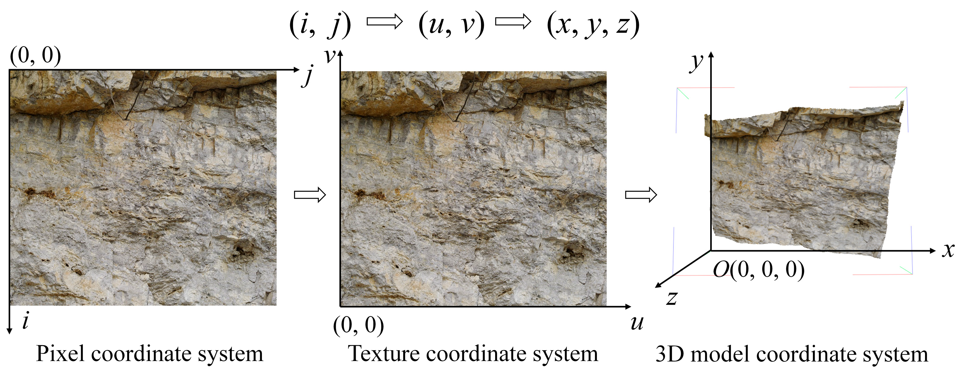
The fractures and cavities vector graphics are saved as 2D pixel coordinates, which cannot be overlaid on the digital outcrop texture model in batch. Therefore, to incorporate the 2D geological information into the 3D digital outcrop model, the 2D pixel coordinates of the contour vertices of the vector graphics must be converted into 3D model coordinates. The DOM is essentially a triangular mesh surface model. If the transformation between each triangle surface in the model skeleton and its corresponding triangular surface in the texture coordinate system is considered an orthographic projection, affine transformation may be used to approximately invert this projection connection. Based on this, we may project any point in the model’s texture picture onto the DOM’s surface. The projection transformation method for each vertex in a 2D graphics contour consists of two steps (Figure 3): (1) 2D pixel coordinates to 2D texture coordinates; (2) 2D texture coordinates to 3D model coordinates.
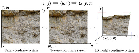
Figure 3.
The overall process to project 2D vector graphics to 3D graphics.
3.3.1. Translating 2D Pixel Coordinates to 2D Texture Coordinates
The origin of the pixel coordinate system is the upper left corner of the outcrop picture, where i denotes the row number and j denotes the column number in the pixel coordinate system. The coordinate origin of the texture coordinate system is in the lower-left corner of the texture picture. The texture coordinate system’s abscissa is u, and the ordinate is v, with u and v values ranging from 0 to 1. Formula (1) depicts the link between the pixel coordinate system and the texture coordinate system. The pixel coordinates of the detected fractures and cavities graphics contour vertices may be translated into texture coordinates using Formula (1).
where h is the height of the outcrop picture and w is its width.
3.3.2. Translating 2D Texture Coordinates to 3D Model Coordinates
To project the graphics in the texture coordinate system onto the 3D digital outcrop, we utilize affine transformation to infer the mapping connection between each triangle in the model skeleton and its corresponding triangle in the texture space. For any pair of triangle faces in two vector spaces, the 3D model coordinates (x, y, and z) and 2D texture coordinates (u, v) of all vertices are saved in the model file. Based on this, the mapping connection between the two triangular surfaces can be constructed, and each vertex included in the texture triangular surface may be projected onto the corresponding triangular surface in 3D space. Assuming that there is a point t (u, v) in the texture space triangle ∆ (t1, t2, t3) (Figure 4b), it is now projected into the 3D space triangle ∆ (p1, p2, p3), and the projection result is stored as p (x, y, z) (Figure 4a). To simplify the computation, first rotate the 3D coordinate system about the origin such that a coordinate axis coincides with the direction of the ∆ (p1, p2, p3) triangle’s normal vector, forming a local 3D coordinate system. A specific method for establishing a local coordinate system is described in Figure 4a. To create the Y-axis of the local coordinate system, rotate the y-axis of the original coordinate system to the direction, which corresponds to the direction of the normal vector of the ∆ (p1, p2, p3) triangle. Then, rotate the z-axis of the original coordinate system to the direction coinciding with the ∆ (p1, p2, p3) triangle’s edge p1p2 to obtain the z-axis of the local coordinate system. Finally, the direction perpendicular to the plane ZOY is chosen as the local coordinate system’s x-axis direction. Formula (2) depicts the transformation connection between global 3D coordinates and local 3D coordinates.
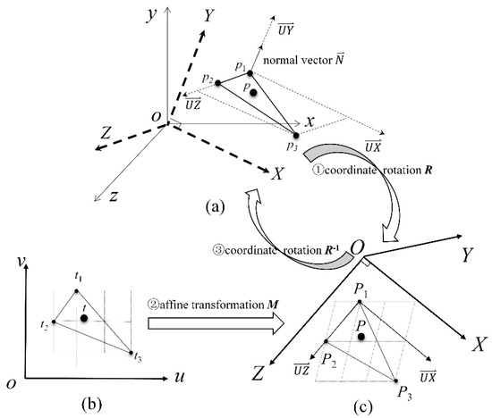
Figure 4.
Schematic diagram of the process of converting 2D texture coordinates to 3D model coordinates. (a) 3D coordinate system. (b) Texture coordinate system. (c) Local 3D coordinate system.
The rotation matrix R can be expressed by three unit vectors consistent with the x, y, and z axes of the local coordinate system (Formula (3)).
Formula (4) depicts the procedure for calculating , , and .
On the other hand, by calculating the inverse matrix R−1 of R, the local 3D coordinates may be translated into global 3D coordinates (Formula (5)).
After the rotation transformation, the corresponding points of the three vertices p1(x1, y1, z1), p2(x2, y2, z2), and p3(x3, y3, z3) of the triangle ∆ (p1, p2, p3) in the local 3D coordinate system can be obtained, which are recorded as P1(X1, Y1, Z1), P2(X2, Y2, Z2), and P3(X3, Y3, Z3). The Y value of all points on the triangle surface ∆ (P1, P2, P3) is a constant Y0, Y1 = Y2 = Y3 = Y0, since the local coordinate system’s Y-axis is perpendicular to the triangular surface ∆ (P1, P2, P3). Therefore, the mapping relationship between the triangular surface ∆ (P1, P2, P3) and its corresponding triangular surface ∆ (t1, t2, t3) in the texture coordinate system can be regarded as an affine transformation between two 2D triangular surfaces (Figure 4b,c).
Affine transformation is a geometric transformation that involves a linear transformation (scaling and rotation) followed by a translation transformation to change a vector space into another vector space. The vector is rotated, scaled A, and translated to obtain the vector (Formula (6)).
The homogeneous coordinate expression of affine transformation matrix M is as follows:
As a result, Formula (8) may be used to define the mapping connection between point t in 2D texture coordinate space and point P in local 3D coordinate space.
The local 3D coordinates and texture coordinates of the triangle’s three vertices are brought into Formula (8) for each pair of triangular surfaces in texture space and 3D space, and the unknown parameters a, b, c, d, m, and n may be solved. The affine transformation matrix M is obtained at this point. The texture space point t is then entered into Formula (8) to calculate the local 3D coordinates P(X, Y0, Z), where Y0 is a constant obtained in Formula (2). The point t is projected into the local three-dimensional space. Finally, the global 3D coordinates p(x, y, z) are obtained by plugging P(X, Y0, Z) into Formula (5).
3.4. Seamless Superposition of 3D Vector Graphics and DOM
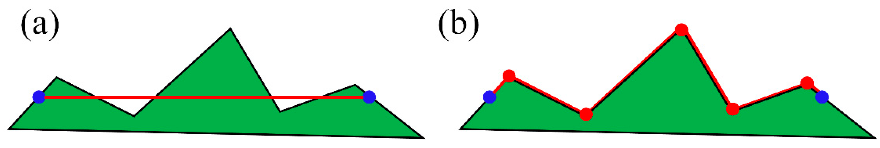
If the approach proposed in Section 3.3 is used directly to project the 2D graphics of the fractures and cavities into 3D space, the generated 3D graphics will not entirely fit the DOM surface, and the graphics will be suspended or pierce the model. The obtained 3D graphics cannot accurately describe the real shape and size of fractures and cavities (Figure 5a). Therefore, we first reconstruct fractures and cavities based on the geometric geometry of the triangular mesh. Then we convert the 2D pixel coordinates of the reconstructed graphics into 3D model coordinates, so that the 3D graphics of fractures and cavities can fit on the model surface (Figure 5b).
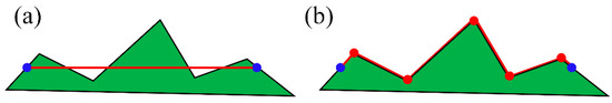
Figure 5.
Schematic diagram of reconstruction of fracture-cavity graphics. In (a), the red line represents the line segment between any two points on the contour of the fractures or cavities, and the blue point is the two vertices of the line segment. If only the blue vertices of the contour edge are converted to the model surface, the red line segment does not fully fit the model. In (b), the red line is reconstructed to generate multiple red points. By connecting all points, the graphics fit perfectly with the model surface.
3.4.1. 2D Vector Graphics Reconstruction
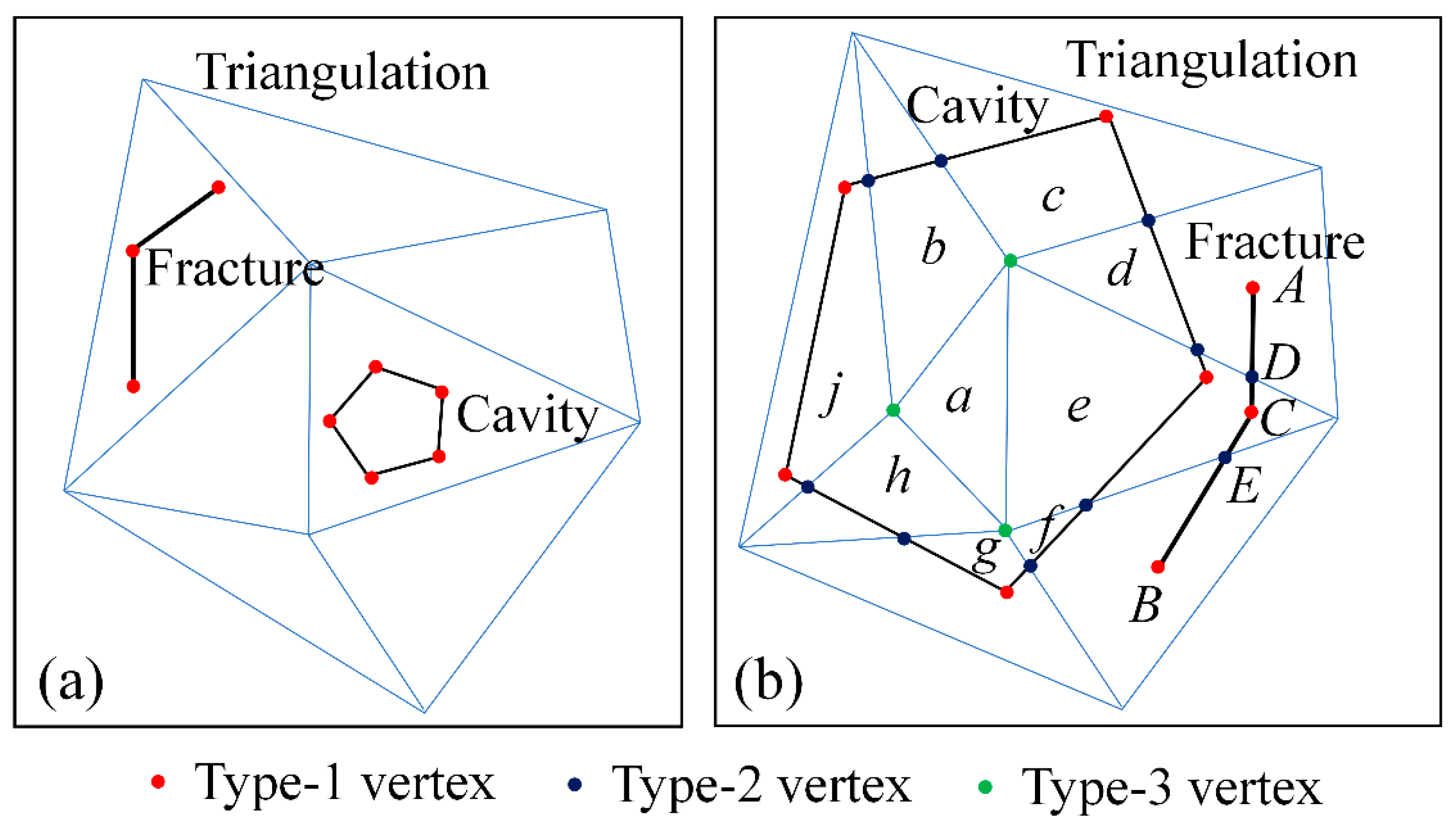
The reconstruction of fractures and cavities graphics in 2D texture space can be realized by superposition and intersection of graphics and covered triangular network. A schematic representation of superposition intersection is shown in Figure 6. There are two possibilities. (1) When the coverage of a single fracture or cavity is so small that it is completely contained in a triangle in the triangulation, there is no need for reconstruction (Figure 6a). (2) On the contrary, if a single fracture or cavity covers multiple triangles in the mesh, the covered triangles need to be used to reconstruct the graph. We use the methods of superposition of line and triangulation and superposition of polygon and triangulation to realize fracture reconstruction and cavity reconstruction, respectively. By triangulation, the cavity polygon in Figure 6b is divided into multiple arbitrary polygons: a, b, c, d, e, f, g, h, and i. Multiple vertices are acquired after the intersection of the fracture and the triangulation: A, D, C, E, and B. The superposition and intersection of vector graphics is a common algorithm in the fields of computational geometry and GIS, and many mature solutions have been proposed [54,55,56]. This study focuses on Liu’s algorithm [56] for realizing geometric figure intersections; therefore, the precise stages are not repeated.
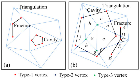
Figure 6.
The intersection of the triangulation and the geometries of the fractures and cavities. (a) The fracture or cavity in the interior of a triangle; (b) the fracture or cavity covers multiple triangles.
3.4.2. Seamless 3D Rendering
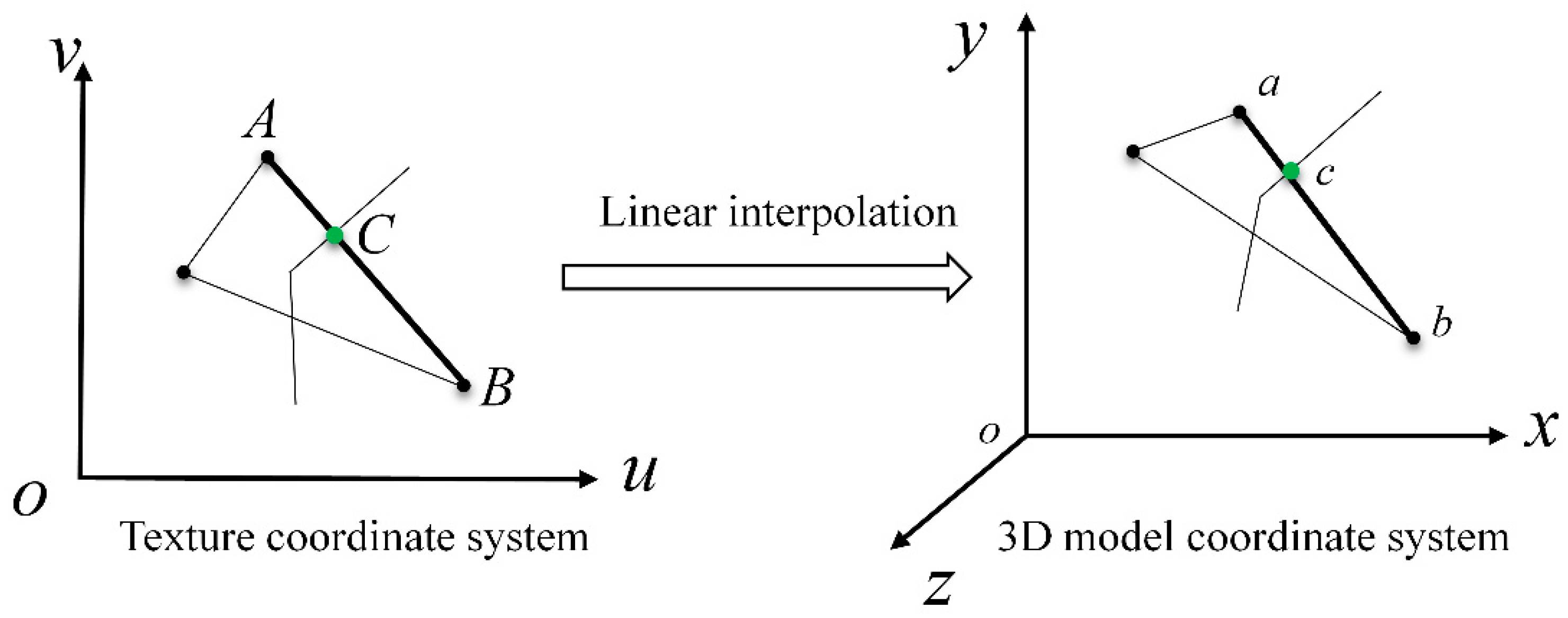
The reconstructed graph’s vertices may be classified into three groups (Figure 6). By using different methods to convert the vertices to 3D space, the seamless overlapping rendering of these vector graphics on the outcrop surface can be realized. Type-I vertices are vertices existing before reconstruction. We use the projection method introduced in Section 3.3 to solve its 3D model coordinates. The vertex of triangulation of the DOM is known as Type-II vertices, and its 3D model coordinates are known as well. Type-III vertices are newly generated points in the process of superposition and intersection, and their 3D model coordinates can be calculated by linear interpolation. It is assumed that there is a type-III vertex C in the texture space, which is positioned on an edge AB, as illustrated in Figure 7. The corresponding edge of AB edge in 3D space is ab, and the 3D coordinates of the two ends of edge ab are a (x1, y1, z1) and b (x2, y2, z2), respectively. If the transformation from edge AB to edge ab is regarded as a linear transformation, the coordinates of the corresponding point c (x0, y0, z0) of point C in the 3D coordinate system can be solved by Formula (9).
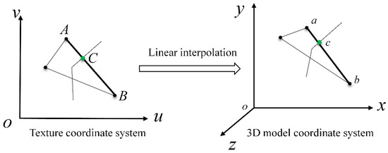
Figure 7.
The idea of the method to calculate 3D coordinates of intersections using linear interpolation.
3.5. Automated 3D Statistical Analysis
So far, we obtain the 3D polylines of the fractures contour and the 3D surfaces of the cavities. The 3D polylines are the trace of two intersecting planes: the surface of the DOM and the plane of the fractures. The fractures (3D polylines) and cavities (3D surfaces) may be quantitatively described after acquiring an accurate 3D representation on the DOM. By calculating the related indicators (length, area, etc.) of fractures and cavities and combining them with the DOM, we attempt to further analyze the distribution features of fractures and cavities in the research region. The characteristic parameters of fractures distribution include quantity, density, average length, total length, and average orientation. The calculation of the length and orientation of a single fracture is the basis for other parameters. Since the 3D model coordinates of fracture vertices have been obtained, the distance between two adjacent vertices on a single fracture can be calculated in turn, and the sum is the length of the fracture. In addition, we fit the direction of the fracture vertex set to identify the precise orientation of the fracture using the principal component analysis approach described in the literature [57,58]. The characteristic parameters of cavities distribution include quantity, density, total area, and average area. The calculation of the area of a single cavity is the basis for other indicators. As described in 3.4.1 of this paper, the cavity polygon is reconstructed to form a composite polygon composed of multiple arbitrary polygons, which can fit seamlessly with DOM. The surface area of a cavity is calculated by adding the areas of all arbitrary polygons that make up the cavity.
4. Results and Discussion
4.1. Method Implementation
The feature detection algorithm of fractures and cavities has been discussed in detail in the literature [24,27], and its efficiency and effect are worthy of affirmation. Therefore, in Windows 10 environment, this paper carries out experiments through the algorithm in Section 3.3, Section 3.4 and Section 3.5. Using C++ programming language and 3D visualization open source library (OSG), the author realizes the related algorithms and 3D visualization of fractures and cavities graphics. Figure 8 is a test effect figure of the implemented algorithm on a test model. In Figure 8a, the 3D graphics of fractures and cavities are accurately fitted on the test model surface. Figure 8b shows the rendering effect of vector lines (fractures lines) on the DOM, and the fractures lines are closely attached to the triangular surface. There are no abnormalities of aliasing, suspension, and penetration. Figure 8c shows the rendering effect of vector surface (cavities) on the framework model. The edge of the face is precisely cut in this figure, and the interior of the face suits the model perfectly.
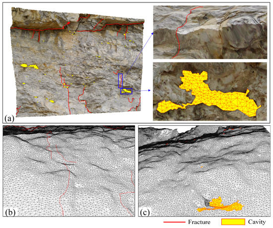
Figure 8.
3D Rending results of fractures and cavities: (a) Overall effect; (b) polylines (fractures); (c) polygons (cavities) rendering over the skeleton model.
The execution time of the overall algorithm is closely related to the scale of the model and the number of fractures and cavities graphics. The number of triangular surfaces in the test model utilized in this paper reaches 169,260, with a textured image size of 7264 × 5440. In the model, there are a total of 820 graphics of fractures and cavities. The following is the test environment of the algorithm used: the CPU is Intel ® Core ™ I5-10400, the main frequency is 2.9 GHz, and the graphics card is Intel® UHD Graphics 630 with 16.0 GB memory. The algorithm’s entire execution time is 5.6 s, which is acceptable to the user. It demonstrates that the operation efficiency of the algorithm described in this paper can meet the application requirements.
4.2. Case Study
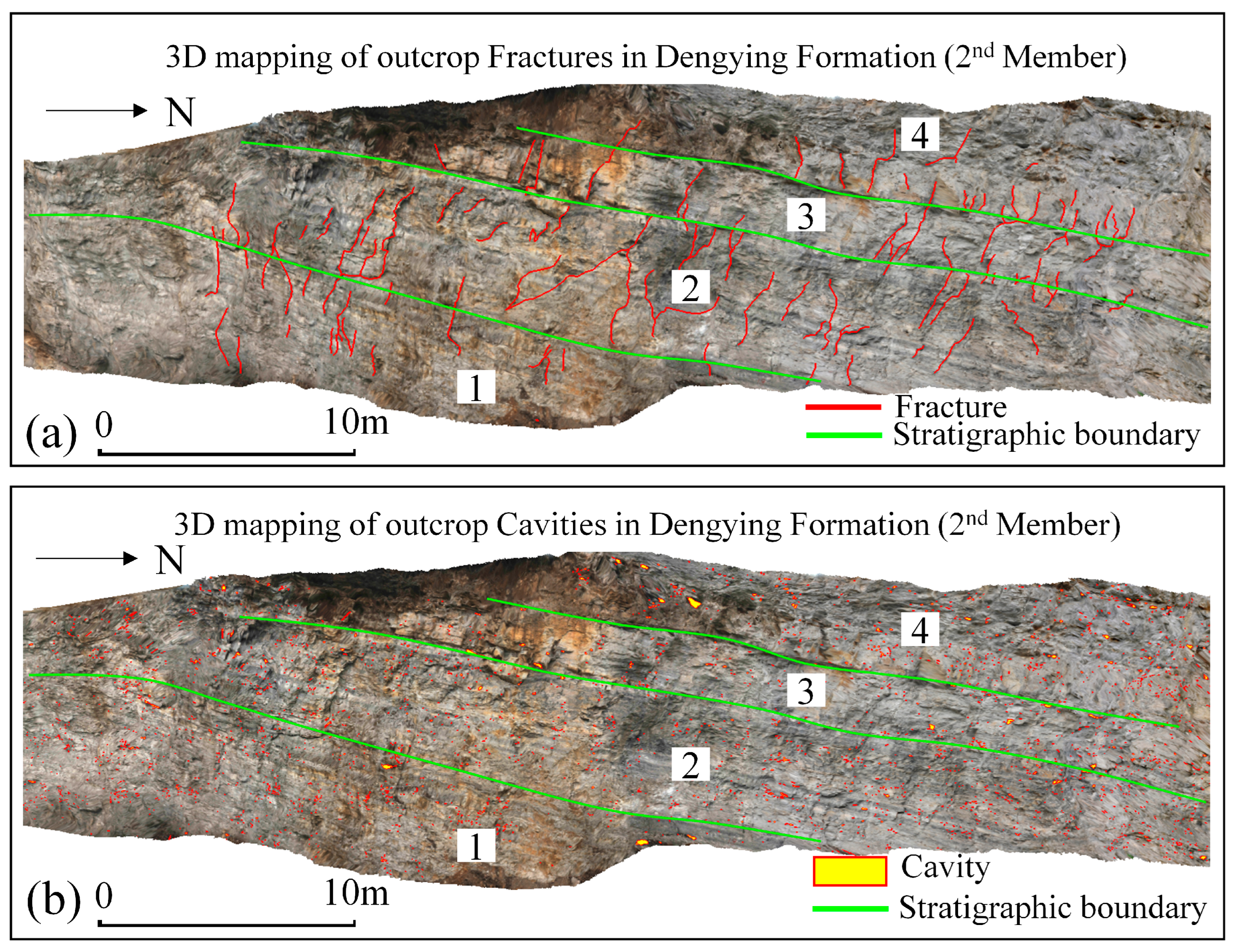
In this section, the proposed method is applied to the 3D mapping and quantitative characterization of fractures and cavities graphics on the outcrop profile for the Dengying Formation (second member). A total of 7586 cavities are automatically extracted from the outcrop texture image by using the deep learning algorithm [24]. We detect the fractures in the study area through the corresponding detection methods [27]. The detection approach has some reliability, as described in the references [27], but the automatic detection method may also be enhanced. Firstly, we use this method to detect fractures. Then, we manually optimize the detection results, and finally obtain 261 fractures. Then, these fractures and cavities graphics are mapped to the 3D model by using the method proposed in this paper, and the seamless rendering of geological information of fractures and cavities on 3D digital outcrop is realized (Figure 9).
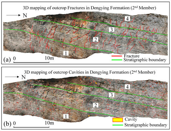
Figure 9.
3D visualization of fractures and cavities of the Dengying Formation (second member). (a) 3D visualization of fractures. (b) 3D visualization of cavities.
The fractures (3D polylines) and cavities (3D surfaces) scale parameters (fracture length and cavity area, etc.) can be calculated automatically in 3D space when the 3D mapping of fractures and cavities graphics is completed. These parameters include density: surface density of fractures (density = number of 3D polylines/surface area of outcrop), total length: the total length of the fractures, average length: the average length of the fractures, average orientation: the average angle formed by the intersection of the 3D polyline’s fitting line and the plumb line, total area: the total surface area of cavities, average cavity area: the average surface area of cavities, surface porosity (surface porosity = the total surface area of cavities/the surface area of outcrop), etc. (Table 1). Thus, the structure and distribution characteristics of the graphics of fractures and cavities on the outcrop surface are further counted by layers.

Table 1.
Statistics of fracture-cavity characteristic parameters of the Dengying Formation (second member).
According to the number, density, average length, total length, and average orientation of fractures calculated for each layer (Table 1), there are differences in the development of fractures in the four layers. Layers 1 and 3 have a higher surface density (fractures) than the other layers. Layer 2 has the largest outcrop surface area and contains the most fractures. The number and density of fractures are the lowest in layer 4. There are intersecting fractures on the outcrop surface. The average included angle between layer 1’s fractures and the plumb line is the lowest. The direction of the fractures on the outcrop surface is close to the plumb line. The author makes an overall and layered analysis of the fractures, revealing that the average orientation of the fractures is 18°. The fractures are stratified differently, with the lower layer having more vertical fractures, and the overall direction is similar. The following is the distribution characteristics of the Dengying Formation (second member): layers 1–4 have a surface porosity of 0.56% to 0.76%, with layer 4 having the highest surface porosity (0.76%) and layer 1 having the lowest surface porosity (0.56%). The development density of cavities is between 15–26 numbers/m2. Among them, many small cavities exist in layers 1 and 2, with a small average area and dense spatial distribution; many huge cavities exist in layers 3 and 4, with a large average area and sparse spatial distribution. The maximum cavity area of layer 4 is 21,902 mm2, the median cavity area is 162 mm2, the maximum cave perimeter is 841.29 mm, and the median cavity perimeter is 51.31mm. The characteristic genesis of the cavities in layer 4 is that they are close to the top interlayer weathering crust.
The main content of this research includes three parts. (1) The contours of fractures and cavities are detected on the photos. (2) The contours of 2D fractures and cavities are mapped to the surface of DOM. Then, the 3D polylines of the fracture contour and the surface of the cavity are further obtained. (3) We calculate the 3D features of 3D polylines and cavity surfaces. We are committed to studying how to display the fractures and cavities detected in the photos on the DOM surface. This is the focus of this paper. However, we can only obtain the trace lines of fractures and cavities on the outcrop surface. So, we can only calculate the parameters (length and orientation, etc.) of the 3D polylines. In future, we will compare 2D fractures and cavities with automatically mapped 3D fractures and cavities, and we will attempt to calculate a best-fitting plane of the fracture and count the fracture characteristics (dip direction, dip angle, etc.) based on [59], which is likely to have interesting results for geologists. At this stage, we still lack enough data for more in-depth analysis, such as the prediction of conduit porosity at different scales [60]. We will further improve the relevant research in the follow-up work.
5. Conclusions
This research proposes a scheme for 3D quantitative characterization of fractures and cavities in the digital outcrop texture model based on lidar. The authors use this method to implement 3D mapping of fractures and cavities graphics in the profile of Dengying Formation (second member). Further parameter characterization and statistical analysis of fractures and cavities elements are carried out based on the 3D mapping results. The achievements and understanding are as follows:
- (1)
- Combined with lidar and digital photography, a high-resolution 3D DOM of the profile of Dengying Formation (second member), Sichuan Basin is established. Based on the outcrop image, the fractures and cavities on the outcrop surface are automatically extracted.
- (2)
- We proposed a new method for 3D visualization of 2D vector geological information in the DOM. Firstly, the 2D fractures and cavities vector graphics are superimposed and intersected with the triangular network in the texture coordinate system. At this time, the 2D vector graphics are reconstructed. Then, based on geometric transformations such as affine transformation and linear interpolation, the fractures and cavities graphics in texture space are projected onto the surface of 3D model. Thus, the seamless rendering of vector fractures and cavities geological information in digital outcrop is realized.
- (3)
- The characteristics of fractures and cavities on the section of Dengying Formation (second member), Sichuan Basin are characterized in 3D space, and the characteristic parameters of various fractures and cavities are counted by layers. The results provide a basis for reservoir evaluation on this section.
The proposed method can realize fine characterization of macro geological structure characteristics on the 3D digital outcrop profile. It enhances the practicability of the 3D DOM by providing technical conditions for quantitative interpretation of various geological features in the DOM. The detection and study of geological characteristics on the DOM are beneficial to oil and gas exploration and development. Compared with traditional manual interpretation methods, the proposed method has higher efficiency and operability and is expected to become a conventional method for 3D digital outcrop characterization.
Author Contributions
Conceptualization, B.L. and Y.L.; methodology, Y.L. and B.L.; software, Y.L. and B.L.; validation, Q.W. and S.L.; formal analysis, S.L.; writing—original draft preparation, B.L, Y.S., and N.Z.; writing—review and editing, Y.L. All authors have read and agreed to the published version of the manuscript.
Funding
This research was funded by the National Natural Science Foundation of China (No. 41701537, No. 42172172); The Opened-end Fund of State Key Laboratory of Geo-Information Engineering of China (SKLGIE2016-Z-4-1; SKLGIE2017-M-4-6); China Petroleum Science & Technology Innovation Fund (Differential diagenetic evolution and pore development mechanism of continental mixed shale oil, Xixin Wang).
Institutional Review Board Statement
Not applicable.
Informed Consent Statement
Not applicable.
Data Availability Statement
Data available from the authors upon request.
Acknowledgments
The authors would like to express their gratitude to the PetroChina Research Institute of Petroleum Exploration & Development for providing the resources required to collect the samples used in this study. Additionally, special thanks go to the editor and anonymous reviewers for their constructive comments that substantially improve the quality of the paper.
Conflicts of Interest
The authors declare no conflict of interest.
References
- Vest Sørensen, E.; Pedersen, A.K.; García-Sellés, D.; Strunck, M.N. Point clouds from oblique stereo-imagery: Two outcrop case studies across scales and accessibility. Eur. J. Remote Sens. 2015, 48, 593–614. [Google Scholar] [CrossRef] [Green Version]
- Burnham, B.S.; Hodgetts, D. Quantifying spatial and architectural relationships from fluvial outcrops. Geosphere 2019, 15, 236–253. [Google Scholar] [CrossRef] [Green Version]
- Marques, A., Jr.; Horota, R.K.; de Souza, E.M.; Kupssinskü, L.; Rossa, P.; Aires, A.S.; Bachi, L.; Veronez, M.R.; Gonzaga, L., Jr.; Cazarin, C.L. Virtual and digital outcrops in the petroleum industry: A systematic review. Earth-Sci. Rev. 2020, 208, 103260. [Google Scholar] [CrossRef]
- Fabuel-Perez, I.; Hodgetts, D.; Redfern, J. A new approach for outcrop characterization and geostatistical analysis of a low-sinuosity fluvial-dominated succession using digital outcrop models: Upper Triassic Oukaimeden Sandstone Formation, central High Atlas, Morocco. AAPG Bull. 2009, 93, 795–827. [Google Scholar] [CrossRef]
- Viana, C.D.; Endlein, A.; Campanha, G.A.D.C.; Grohmann, C.H. Algorithms for extraction of structural attitudes from 3D outcrop models. Comput. Geosci. 2016, 90, 112–122. [Google Scholar] [CrossRef]
- Jones, R.R.; McCaffrey, K.J.; Clegg, P.; Wilson, R.W.; Holliman, N.S.; Holdsworth, R.E.; Imber, J.; Waggott, S. Integration of regional to outcrop digital data: 3D visualization of multi-scale geological models. Comput. Geosci. 2009, 35, 4–183. [Google Scholar] [CrossRef]
- Cao, T.; Xiao, A.; Wu, L.; Mao, L. Automatic fracture detection based on Terrestrial Laser Scanning data: A new method and case study. Comput. Geosci. 2017, 106, 209–216. [Google Scholar] [CrossRef]
- Buckley, S.J.; Enge, H.D.; Carlsson, C.; Howell, J.A. Terrestrial laser scanning for use in virtual outcrop geology. Photogramm. Rec. 2010, 25, 225–239. [Google Scholar] [CrossRef]
- Becker, I.; Koehrer, B.; Waldvogel, M.; Jelinek, W.; Hilgers, C. Comparing fracture statistics from outcrop and reservoir data using conventional manual and t-LiDAR derived scanlines in Ca2 carbonates from the Southern Permian Basin, Germany. Mar. Petroleum Geol. 2018, 95, 228–245. [Google Scholar] [CrossRef]
- Wang, X.; Gao, F. Quantitatively deciphering paleostrain from digital outcrops model and its application in the eastern Tian Shan, China. Tectonics 2020, 39, e2019TC005999. [Google Scholar] [CrossRef]
- Kong, D.; Saroglou, C.; Wu, F.; Sha, P.; Li, B. Development and application of UAV-SfM photogrammetry for quantitative characterization of rock mass discontinuities. Int. J. Rock Mech. Min. Sci. 2021, 141, 104729. [Google Scholar] [CrossRef]
- Pickel, A.; Frechette, J.; Comunian, A.; Weissmann, G. Building a training image with Digital Outcrop Models. J. Hydrol. 2015, 531, 53–61. [Google Scholar] [CrossRef]
- Huerta, P.; Armenteros, I.; Tomé, O.M.; Gonzálvez, P.R.; Silva, P.G.; González-Aguilera, D.; Carrasco-García, P. 3-D modelling of a fossil tufa outcrop. The example of La Peña del Manto (Soria, Spain). Sediment. Geol. 2016, 333, 130–146. [Google Scholar] [CrossRef]
- Stright, L.; Jobe, Z.; Fosdick, J.C.; Bernhardt, A. Modeling uncertainty in the three-dimensional structural deformation and stratigraphic evolution from outcrop data: Implications for submarine channel knickpoint recognition. Mar. Pet. Geol. 2017, 86, 79–94. [Google Scholar] [CrossRef]
- Wang, X.; Qin, Y.; Yin, Z.; Zou, L.; Shen, X. Historical shear deformation of rock fractures derived from digital outcrop models and its implications on the development of fracture systems. Int. J. Rock Mech. Min. Sci. 2019, 114, 122–130. [Google Scholar] [CrossRef] [Green Version]
- Yan, Y.; Zhang, L.; Luo, X. Modeling Three-Dimensional Anisotropic Structures of Reservoir Lithofacies Using Two-Dimensional Digital Outcrops. Energies 2020, 13, 4082. [Google Scholar] [CrossRef]
- Ren, Q.; Jin, Q.; Feng, J.; Du, H. Design and construction of the knowledge base system for geological outfield cavities classifications: An example of the fracture-cavity reservoir outfield in Tarim basin, NW China. J. Pet. Sci. Eng. 2020, 194, 107509. [Google Scholar] [CrossRef]
- Yeste, L.M.; Palomino, R.; Varela, A.N.; McDougall, N.D.; Viseras, C. Integrating outcrop and subsurface data to improve the predictability of geobodies distribution using a 3D training image: A case study of a Triassic Channel–Crevasse-splay complex. Mar. Petroleum Geol. 2021, 129, 105081. [Google Scholar] [CrossRef]
- Laux, D.; Henk, A. Terrestrial laser scanning and fracture network characterisation–perspectives for a (semi-) automatic analysis of point cloud data from outcrops. Z. Dtsch. Ges. Geowiss. 2015, 166, 99–118. [Google Scholar] [CrossRef]
- Qiao, Z.; Shen, A.; Zheng, J.; Chang, S.; Chen, Y. Three-dimensional carbonate reservoir geomodeling based on the digital outcrop model. Pet. Explor. Dev. 2015, 42, 358–368. [Google Scholar] [CrossRef]
- Corradetti, A.; Tavani, S.; Parente, M.; Iannace, A.; Vinci, F.; Pirmez, C.; Torrieri, S.; Giorgioni, M.; Pignalosa, A.; Mazzoli, S. Distribution and arrest of vertical through-going joints in a seismic-scale carbonate platform exposure (Sorrento peninsula, Italy): Insights from integrating field survey and digital outcrop model. J. Struct. Geol. 2018, 108, 121–136. [Google Scholar] [CrossRef]
- Bertrand, L.; Jusseaume, J.; Géraud, Y.; Diraison, M.; Damy, P.-C.; Navelot, V.; Haffen, S. Structural heritage, reactivation and distribution of fault and fracture network in a rifting context: Case study of the western shoulder of the Upper Rhine Graben. J. Struct. Geol. 2018, 108, 243–255. [Google Scholar] [CrossRef]
- Larssen, K.; Senger, K.; Grundvåg, S.A. Fracture characterization in Upper Permian carbonates in Spitsbergen: A workflow from digital outcrop to geo-model. Mar. Petroleum Geol. 2020, 122, 104703. [Google Scholar] [CrossRef]
- Wang, Q.; Zeng, Q.; Zhang, Y.; Shao, Y.; Wei, W.; Fan, D. Automatic Extraction of Outcrop Cavity Based on Multi-scale Regional Convolution Neural Network. Geoscience 2021, 35, 1147. [Google Scholar]
- Bemis, S.; Micklethwaite, S.; Turner, D.; James, M.R.; Akciz, S.; Thiele, S.T.; Bangash, H.A. Ground-based and UAV-Based photogrammetry: A multi-scale, high-resolution mapping tool for structural geology and paleoseismology. J. Struct. Geol. 2014, 69, 163–178. [Google Scholar] [CrossRef]
- Zeng, Q.; Lu, W.; Zhang, R.; Zhao, J.; Ren, P.; Wang, B. LIDAR-based fracture characterization and controlling factors analysis: An outcrop case from Kuqa Depression, NW China. J. Pet. Sci. Eng. 2018, 161, 445–457. [Google Scholar] [CrossRef]
- Vasuki, Y.; Holden, E.-J.; Kovesi, P.; Micklethwaite, S. A geological structure mapping tool using photogrammetric data. Aseg. Ext. Abstr. 2013, 2013, 1–4. [Google Scholar] [CrossRef] [Green Version]
- Nurshal, M.E.M.; Sadewo, M.S.; Hidayat, A.; Hamzah, W.N.; Sapiie, B.; Abdurrachman, M.; Rudyawan, A. Automatic and manual fracture-lineament identification on digital surface models as methods for collecting fracture data on outcrops: Case study on fractured granite outcrops, Bangka. Front. Earth Sci. 2020, 8, 598. [Google Scholar] [CrossRef]
- Wang, X.; Zou, L.; Shen, X.; Ren, Y.; Qin, Y. A region-growing approach for automatic outcrop fracture extraction from a three-dimensional point cloud. Comput. Geosci. 2017, 99, 100–106. [Google Scholar] [CrossRef] [Green Version]
- Choi, J.; Zhu, L.; Kurosu, H. Detection of cracks in paved road surface using laser scan image data. Int. Arch. Photogramm. Remote Sens. Spat. Inf. Sci. 2016, XLI-B1, 559–562. [Google Scholar] [CrossRef] [Green Version]
- Sun, L.; Kamaliardakani, M.; Zhang, Y. Weighted neighborhood pixels segmentation method for automated detection of cracks on pavement surface images. J. Comput. Civ. Eng. 2016, 30, 04015021. [Google Scholar] [CrossRef]
- Xiao, L.; Zhong, E.; Liu, J.; Song, G.F. A Discussion on Basic Problems of 3D GIS. J. Image Graph. 2001, 6, 842–848. [Google Scholar]
- Guan, L.; Ding, Y.; Zhang, H.; Feng, X.; Tan, X.; Zhao, J. Key Technologies Research and Application of 3D Modeling for Digital City Construction. Bull. Surv. Mapp. 2017, 2, 90–94. [Google Scholar] [CrossRef]
- Vassilaki, D.I.; Stamos, A.A. TanDEM-X DEM: Comparative performance review employing LIDAR data and DSMs. ISPRS J. Photogram. Remote Sens. 2020, 160, 33–50. [Google Scholar] [CrossRef]
- Kourtz, P. Minicomputer production of digital terrain models. Can. J. For. Res. 1983, 13, 343–346. [Google Scholar] [CrossRef]
- Eyton, J.R. Digital elevation model perspective plot overlays. Ann. Assoc. Am. Geogr. 1986, 76, 570–576. [Google Scholar] [CrossRef]
- Minisini, D.; Wang, M.; Bergman, S.C.; Aiken, C. Geological data extraction from lidar 3-D photorealistic models: A case study in an organic-rich mudstone, Eagle Ford Formation, Texas. Geosphere 2014, 10, 610–626. [Google Scholar] [CrossRef] [Green Version]
- Biber, K.; Khan, S.D.; Seers, T.D.; Sarmiento, S.; Lakshmikantha, M. Quantitative characterization of a naturally fractured reservoir analog using a hybrid lidar-gigapixel imaging approach. Geosphere 2018, 14, 710–730. [Google Scholar] [CrossRef]
- Siddiqui, N.A.; Ramkumar, M.; Rahman, A.H.A.; Mathew, M.J.; Santosh, M.; Sum, C.W.; Menier, D. High resolution facies architecture and digital outcrop modeling of the Sandakan formation sandstone reservoir, Borneo: Implications for reservoir characterization and flow simulation. Geosci. Front. 2019, 10, 957–971. [Google Scholar] [CrossRef]
- Alfarhan, M.S.; Alhumimidi, M.S.; Cline, J.R.; White, L.S.; Aiken, C.L. 3D digital photorealistic models from the field to the lab. Arab. J. Geosci. 2020, 13, 1–16. [Google Scholar] [CrossRef]
- Fabuel-Perez, I.; Hodgetts, D.; Redfern, J. Integration of digital outcrop models (DOMs) and high resolution sedimentology–workflow and implications for geological modelling: Oukaimeden Sandstone Formation, High Atlas (Morocco). Pet. Geosci. 2010, 16, 133–154. [Google Scholar] [CrossRef]
- Tavani, S.; Granado, P.; Corradetti, A.; Girundo, M.; Iannace, A.; Arbués, P.; Muñoz, J.A.; Mazzoli, S. Building a virtual outcrop, extracting geological information from it, and sharing the results in Google Earth via OpenPlot and Photoscan: An example from the Khaviz Anticline (Iran). Comput. Geosci. 2014, 63, 44–53. [Google Scholar] [CrossRef]
- Inama, R.; Menegoni, N.; Perotti, C. Syndepositional fractures and architecture of the lastoni di formin carbonate platform: Insights from virtual outcrop models and field studies. Mar. Pet. Geol. 2020, 121, 104606. [Google Scholar] [CrossRef]
- Jin, X.; Song, J.; Liu, S.; Li, Z.; Wen, L.; Sun, W.; Luo, B.; Zhang, X.; Zhou, G.; Peng, H.; et al. Characteristics and geological implications of Dengying Formation tempestites in the periphery of the Sichuan Basin. Nat. Gas Ind. 2021, 41, 11. [Google Scholar]
- Luo, B.; Yang, Y.; Luo, W.J.; Wen, L.; Wang, W.Z.; Chen, K. Controlling factors and distribution of reservoir development in Dengying Formation of paleo-uplift in central Sichuan Basin. Acta Petrolei Sin. 2015, 36, 416–426. [Google Scholar]
- Yang, W.; Wei, G.; Zhao, R.; Liu, M.; Jin, H.; Zhao, Z.; Shen, J. Characteristics and distribution of karst reservoirs in the Sinian Dengying Fm, Sichuan Basin. Nat. Gas Ind. 2014, 34, 50–55. [Google Scholar]
- Yan, Y.; Liu, Y.; Xu, W.; Deng, H.; Luo, W. Necessity to carry out stress experiments on fractured-vuggy carbonate reservoirs under formation conditions: An example from LY gas reservoirs, central Sichuan Basin. Nat. Gas Expl. Dev. 2020, 43, 6. [Google Scholar]
- Yang, Y.M.; Wen, L.; Luo, B.; Xia, M.L.; Sun, S.N. A study of sedimentary characteristics of microbial carbonate: A case study of the Sinian Dengying Formation in Gaomo area, Sichuan Basin. Geol. China 2016, 43, 306–318. [Google Scholar]
- Gu, Y.; Zhou, L.; Jiang, Y.; Jiang, C.; Luo, M.; Zhu, X. A model of hydrothermal dolomite reservoir facies in Precambrian dolomite, Central Sichuan Basin, SW China and its geochemical characteristics. Acta Geol. Sin. (Engl. Ed.) 2019, 93, 130–145. [Google Scholar] [CrossRef] [Green Version]
- Jiang, Y.; Gu, Y.; Zhu, X.; Xu, W.; Xiao, Y.; Li, J. Hydrothermal dolomite reservoir facies in the Sinian Dengying Fm, central Sichuan Basin. Nat. Gas Ind. 2017, 37, 17–24. [Google Scholar] [CrossRef]
- Gu, Y.; Zhou, L.; Jiang, Y.; Ni, J.; Li, J.; Zhu, X.; Fu, Y.; Jiang, Z. Reservoir types and gas well productivity models for Member 4 of Sinian Dengying Formation in Gaoshiti block, Sichuan Basin. Acta PetroleiSinica 2020, 41, 574–583. [Google Scholar]
- Yang, S.; Cheng, H.; Zhong, Y.; Zhu, X.; Chen, A.; Wen, H.; Xu, S.; Wu, C. Microbolit of Late Sinian and its response for Tongwan Movement episode I in Southwest Sichuan, China. Acta Petrol. Sin. 2017, 33, 1148–1158. [Google Scholar]
- Kovesi, P. Image Features from Phase Congruency. J. Comput. Vis. Res. 1999, 1, 1–26. [Google Scholar]
- Bentley, J.L.; Ottmann, T.A. Algorithms for reporting and counting geometric intersections. IEEE Trans. Comput. 1979, 28, 643–647. [Google Scholar] [CrossRef]
- She, J.; Li, C.; Li, J.; Wei, Q. An efficient method for rendering linear symbols on 3D terrain using a shader language. Int. J. Geogr. Inf. Sci. 2018, 23, 476–497. [Google Scholar] [CrossRef]
- Liu, Y.; Sun, Y.; Zhang, K.; Chen, Y. Beijing Da Xue Xue Bao. A Plane Sweep Based Arc Splitting and Polygon Auto-Construction Algorithm. Acta Scientiarum Nat. Univ. Pekin. 2019, 55, 675–682. [Google Scholar]
- Jolliffe, I. Principal component analysis. In Encyclopedia of Statistics in Behavioral Science; John Wiley and Sons Ltd.: New York, NY, USA, 2005. [Google Scholar]
- Wang, X.; Yu, S.; Li, S.; Zhang, N. Two parameter optimization methods of multi-point geostatistics. J. Pet. Sci. Eng. 2022, 208, 109724. [Google Scholar] [CrossRef]
- Albert, G.; Mészáros, J.; Szentpéteri, K. Structural analysis of a Miocene ignimbrite quarry (Tar, Hungary) by Drone (UAV) 3D photogrammetry modelling. In Proceedings of the EGU General Assembly Conference Abstracts, Vienna, Austria, 8–13 April 2018; p. 7310. [Google Scholar]
- Albert, G.; Virág, M.; Eross, A. Karst porosity estimations from archive cave surveys-studies in the Buda Thermal Karst System (Hungary). Int. J. Speleol. 2015, 44, 151. [Google Scholar] [CrossRef] [Green Version]


Publisher’s Note: MDPI stays neutral with regard to jurisdictional claims in published maps and institutional affiliations. |
© 2022 by the authors. Licensee MDPI, Basel, Switzerland. This article is an open access article distributed under the terms and conditions of the Creative Commons Attribution (CC BY) license (https://creativecommons.org/licenses/by/4.0/).