
Application of an Improved STSMC Method to the Bidirectional DC–DC Converter in Photovoltaic DC Microgrid

 , ,
, ,
Abstract
:1. Introduction
2. Operation Mode and Mathematical Modeling of Converter
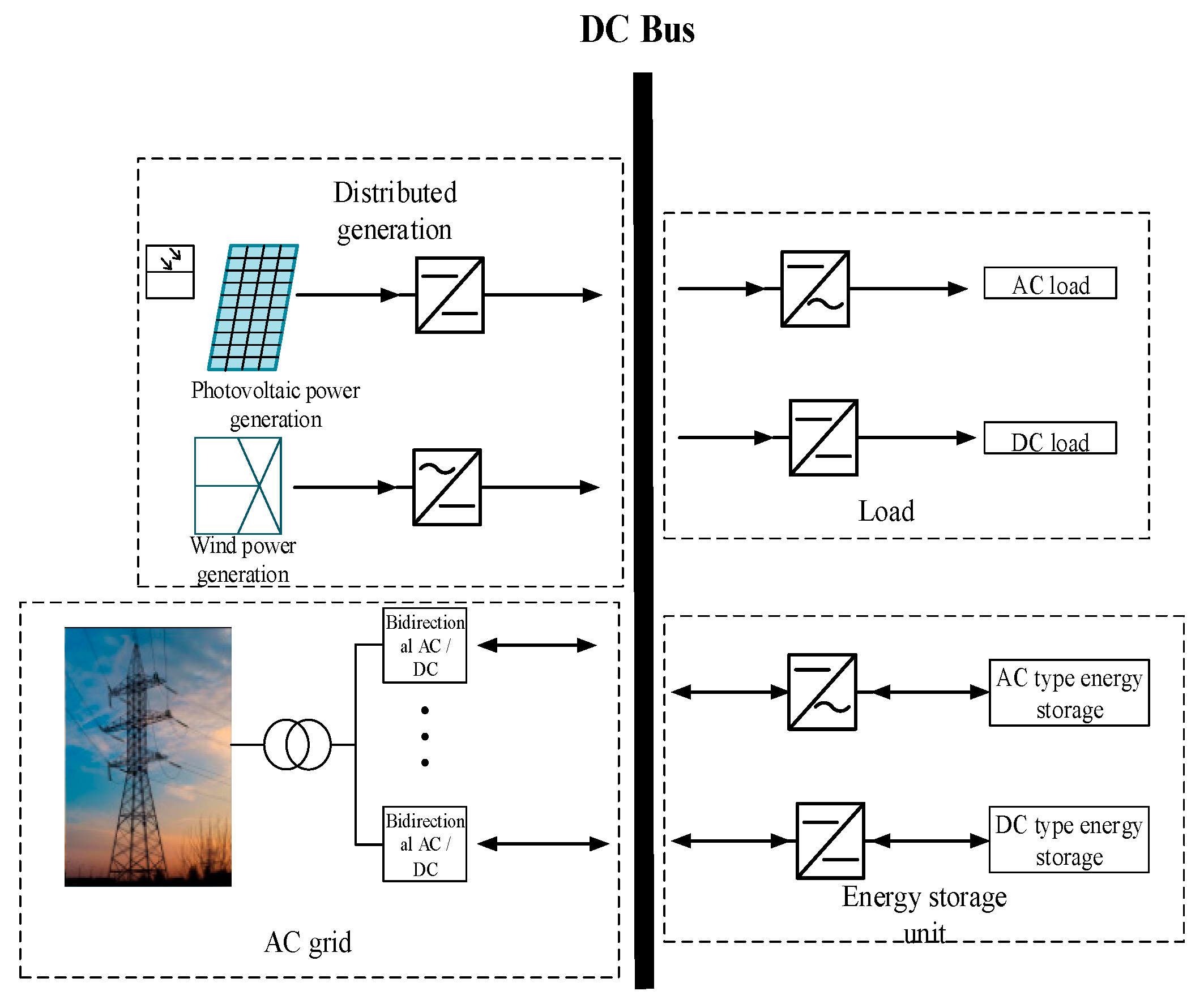
2.1. Photovoltaic DC Microgrid System Structure
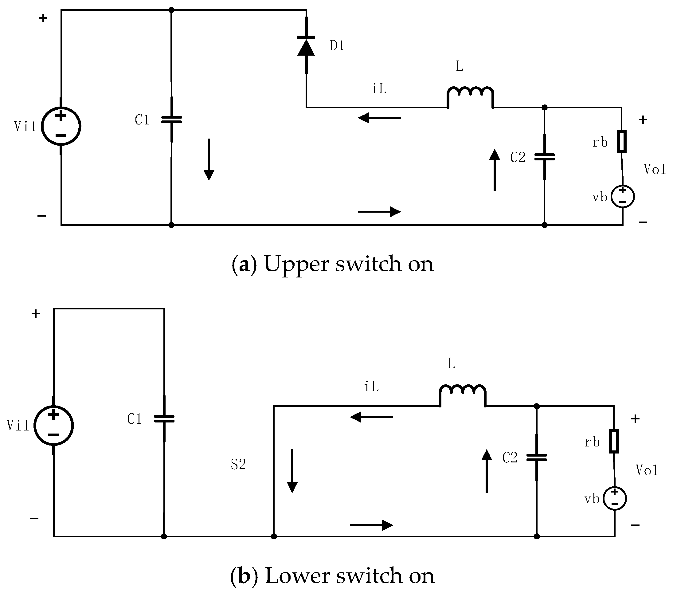
2.2. Topology Selection and Operation Mode
- (1)
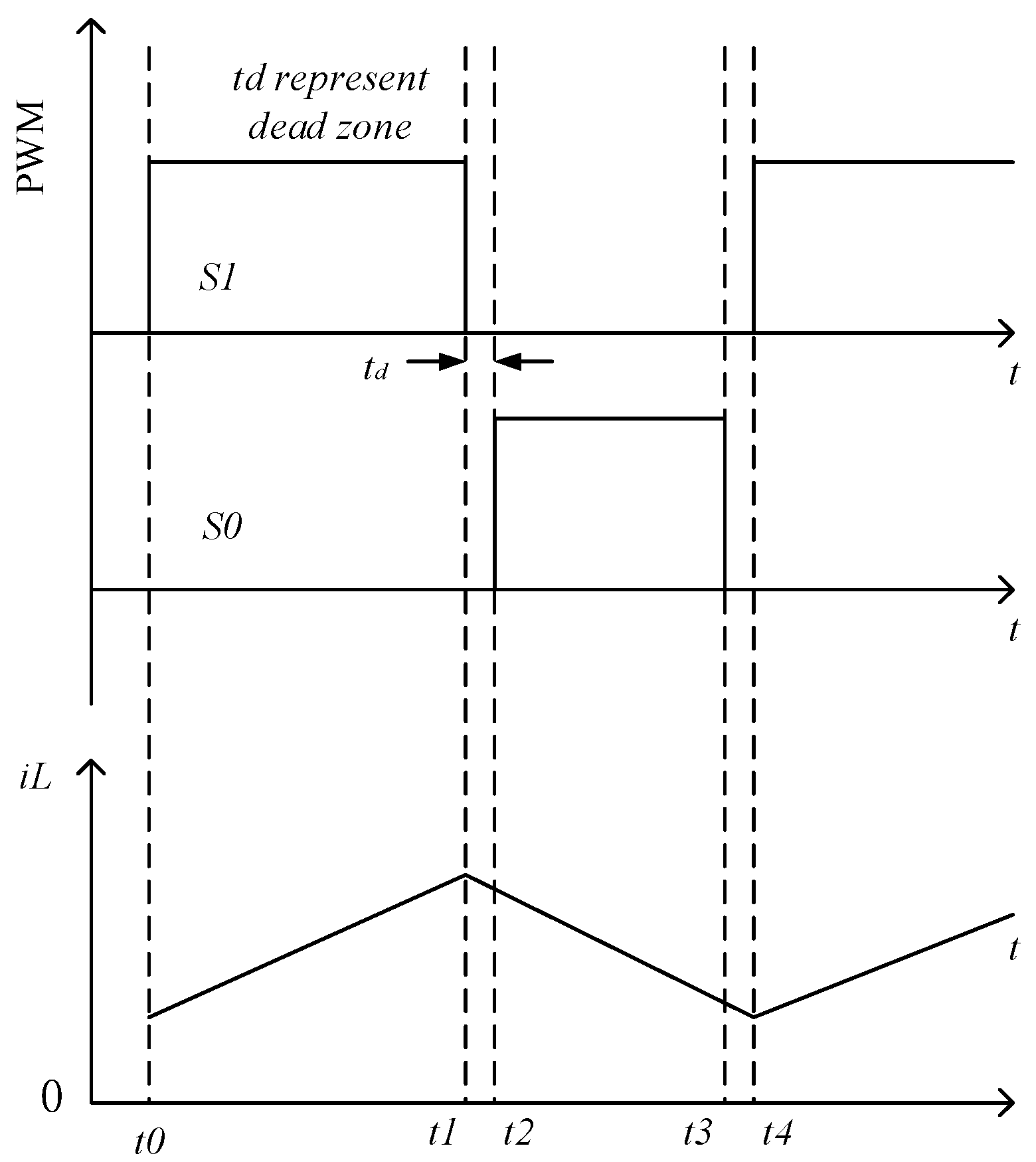
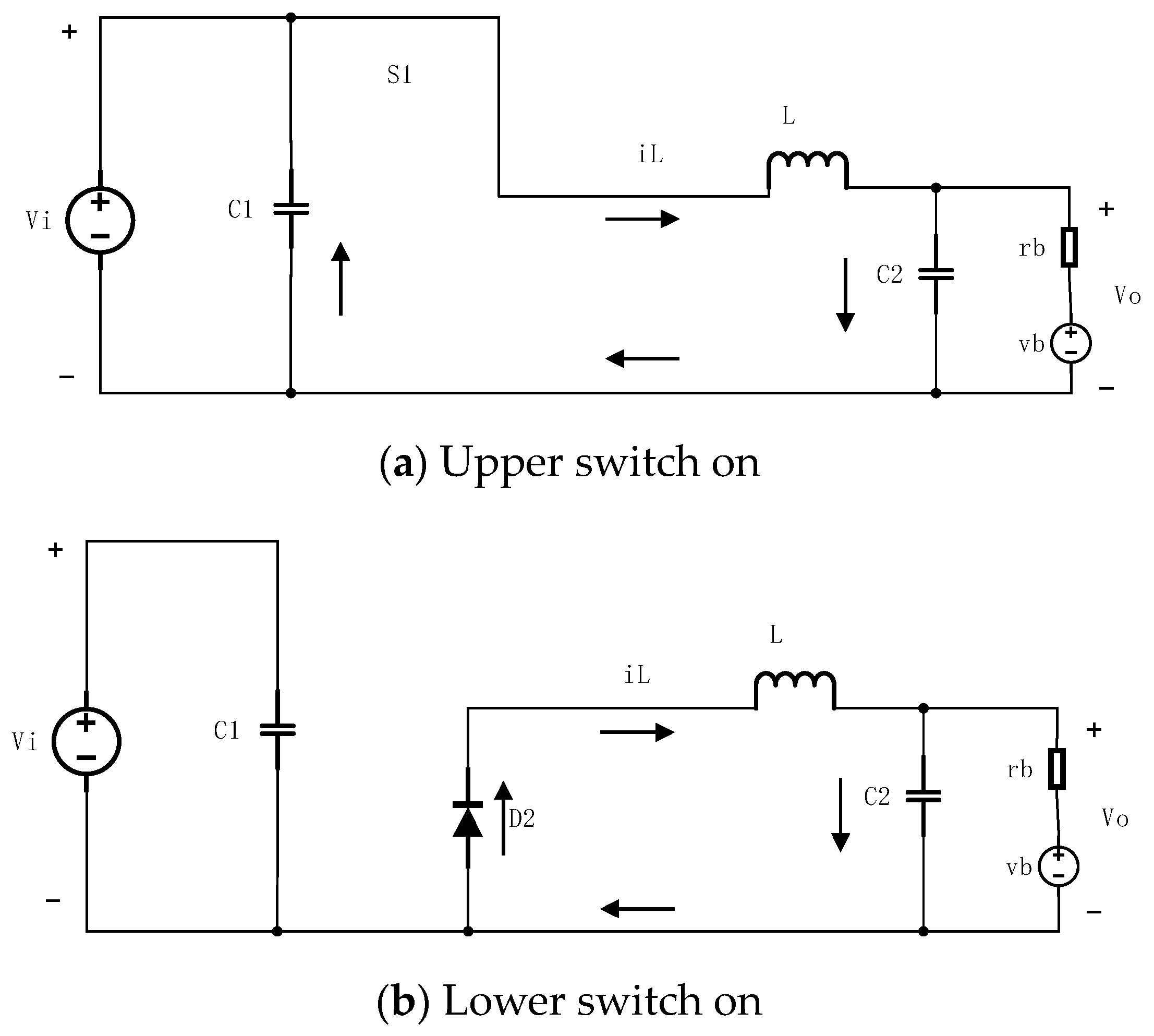
- At t0 − t1, S1 is turned on and S2 is turned off. C2 is being charged and iL increases linearly, as shown in Figure 4a.
- (2)
- At t1 − t2, the circuit works in a dead zone, as shown in Figure 4b, S1 and S2 are turned off, D2 is turned on, and iL begins to decrease.
- (3)
- At t2 − t3, S1 is turned off and S2 applies the driving signal. At this time, D2 is turned on, and iL continues to decrease, as shown in Figure 4b.
- (4)
- At t3 − t4, the circuit returns to the dead zone, so the equivalent circuit is still as shown in Figure 4b. iL continues to decrease. When iL decreases to the minimum, S1 is turned on and starts the next cycle.
- (1)
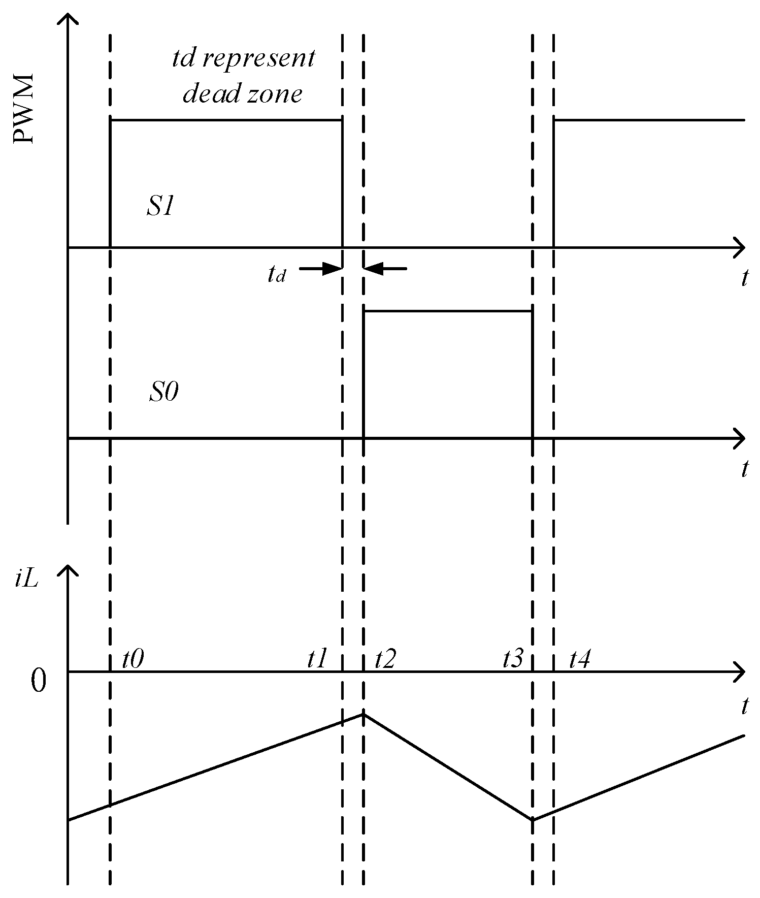
- At t0 − t1, S2 is turned off, S1 applies the driving signal, D1 is turned on, and iL decreases, as shown in Figure 6a.
- (2)
- At t1 − t2, the circuit works in a dead zone, as shown in Figure 6b. S1 and S2 are turned off, D1 is turned on, and iL continues to decrease.
- (3)
- At t2 − t3, the equivalent circuit is shown in Figure 6b. S1 is turned off, S2 is turned on, and iL begins to increase.
- (4)
- At t3 − t4, the circuit returns to the dead zone, so the equivalent circuit is still as shown in Figure 6b. iL begins to decrease and starts to enter the next cycle.
2.3. Modeling of the Bidirectional DC–DC Converter
3. Design of STSMC
3.1. STSMC
3.2. Improved STSMC
3.3. System Stability Analysis
4. Simulation and Results
4.1. Simulation of Proposed Control Method
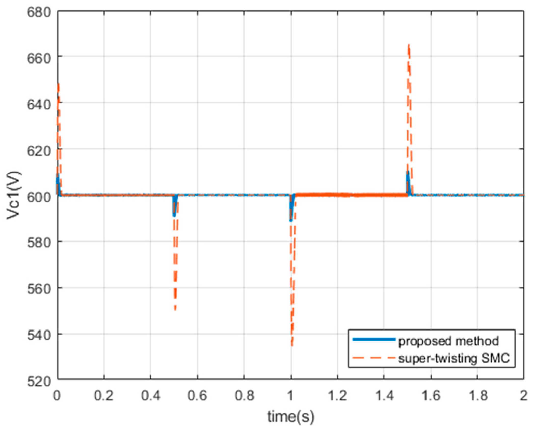
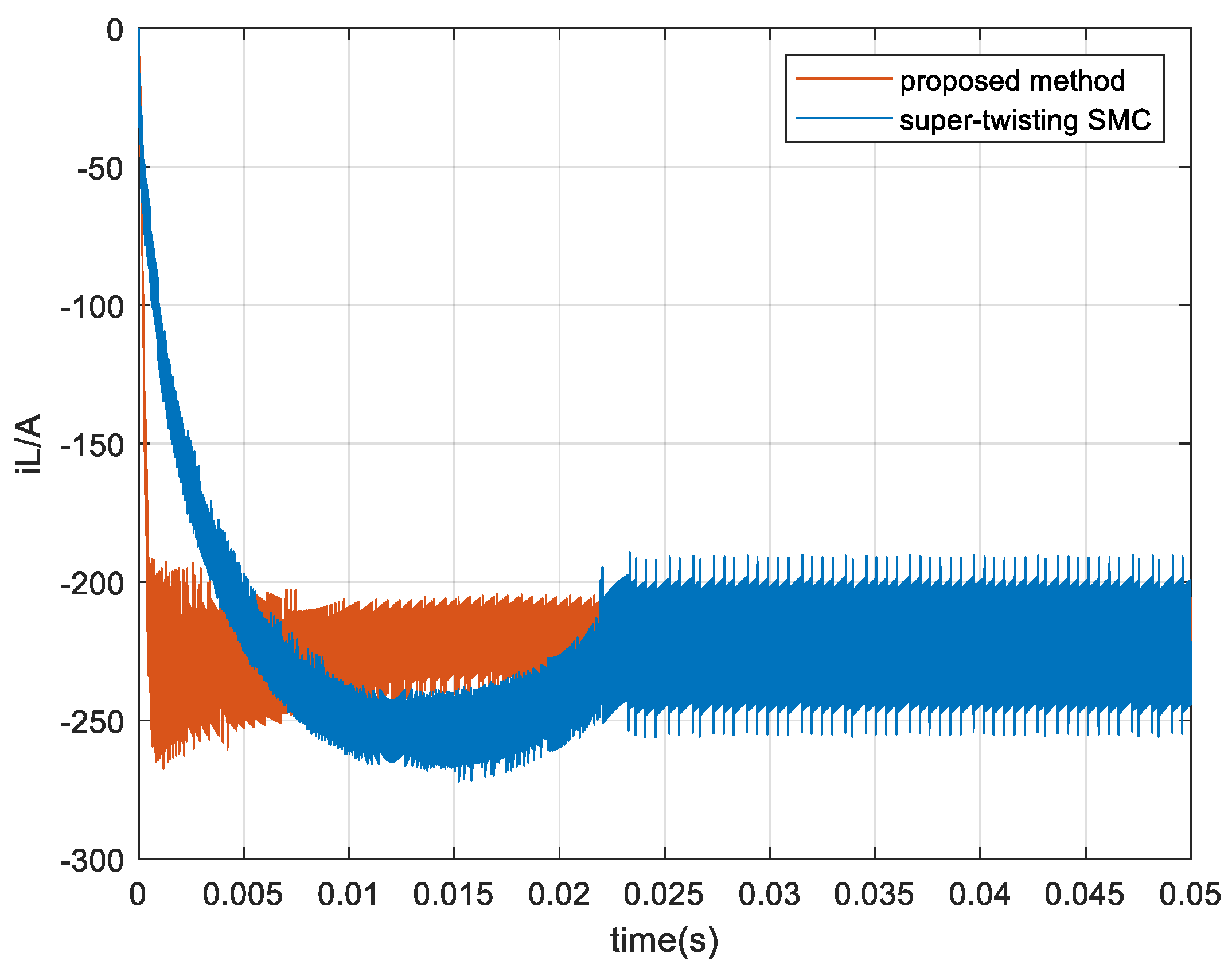
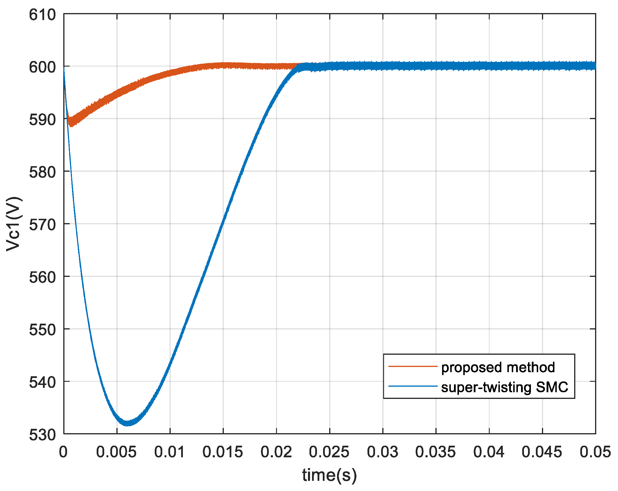
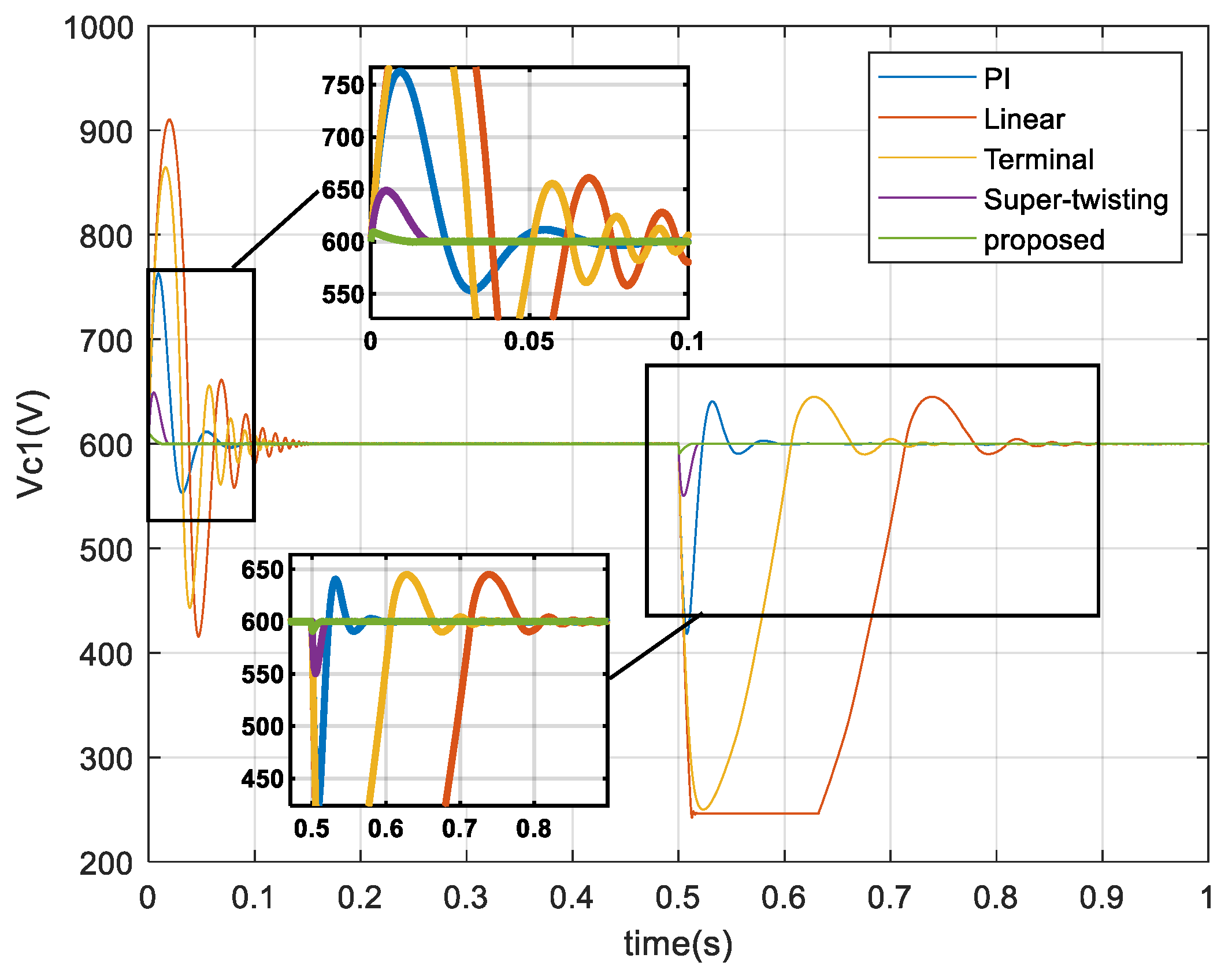
4.2. Performance Comparison
5. Conclusions
Author Contributions
Funding
Institutional Review Board Statement
Informed Consent Statement
Conflicts of Interest
References
- Javaid, N.; Hafeez, G.; Iqbal, S.; Alrajeh, N.; Alabed, M.S.; Guizani, M. Energy Efficient Integration of Renewable Energy Sources in the Smart Grid for Demand Side Management. IEEE Access 2018, 6, 77077–77096. [Google Scholar] [CrossRef]
- Yaseen, M.; Farooq, A.; Malik, M.Z.; Usman, M.; Hafeez, G.; Ali, M. Design of a High Step-Up DC-DC Converter with Voltage Doubler and Tripler Circuits for Photovoltaic Systems. Int. J. Photoenergy 2021, 2021, 1–11. [Google Scholar] [CrossRef]
- Wang, C.; Li, W.; Wang, Y.; Meng, Z.; Yang, L. DC Bus Voltage Fluctuation Classification and Restraint Methods Review for DC Microgrid. Proc. CSEE 2017, 37, 84–98. [Google Scholar]
- Qin, W.P.; Liu, X.S.; Han, X.Q.; Liu, J.Y.; Zhu, X.; Mi, X.D. An Improved Control Strategy of Automatic Charging/Discharging of Energy Storage System in DC Microgrid. Power Syst. Technol. 2014, 38, 1827–1834. [Google Scholar]
- Hosseinzadeh, M.; Salmasi, F.R. Robust Optimal Power Management System for a Hybrid AC/DC Micro-Grid. IEEE Trans. Sustain. Energy 2015, 6, 675–687. [Google Scholar] [CrossRef]
- Sira-Ramirez, H.; Silva-Ortigoza, R. Control Design Techniques in Power Electronic Devices, Power Systems; Springer: London, UK, 2006. [Google Scholar]
- Plestan, F.; Shtessel, Y.B.; Brégeault, V.; Poznyak, A. New methodologies for adaptive sliding mode control. Int. J. Control 2010, 83, 1907–1919. [Google Scholar] [CrossRef] [Green Version]
- Cavallo, A.; Canciello, G.; Guida, B. Supervised control of buck-boost converters for aeronautical applications. Automatica 2017, 83, 73–80. [Google Scholar] [CrossRef]
- Cavallo, A.; Canciello, G.; Russo, A. Integrated supervised adaptive control for the more Electric Aircraft. Automatica 2020, 117, 108956. [Google Scholar] [CrossRef] [Green Version]
- Delghavi, M.B.; Yazdani, A. Sliding-Mode Control of AC Voltages and Currents of Dispatchable Distributed Energy Resources in Master-Slave-Organized Inverter-Based Microgrids. IEEE Trans. Smart Grid 2017, 10, 980–991. [Google Scholar] [CrossRef]
- Zheng, X.; Feng, Y.; Han, F.; Yu, X. Integral-Type Terminal Sliding-Mode Control for Grid-Side Converter in Wind Energy Conversion Systems. IEEE Trans. Ind. Electron. 2018, 66, 3702–3711. [Google Scholar] [CrossRef]
- Li, H.; Wu, W.; Huang, M.; Chung, H.S.-H.; Liserre, M.; Blaabjerg, F. Design of PWM-SMC Controller Using Linearized Model for Grid-Connected Inverter with LCL Filter. IEEE Trans. Power Electron. 2020, 35, 12773–12786. [Google Scholar] [CrossRef]
- Fei, J.; Feng, Z. Fractional-Order Finite-Time Super-Twisting Sliding Mode Control of Micro Gyroscope Based on Double-Loop Fuzzy Neural Network. IEEE Trans. Syst. Man Cybern. Syst. 2020, 51, 7692–7706. [Google Scholar] [CrossRef]
- Lu, J.; Savaghebi, M.; Ghias, A.M.Y.M.; Hou, X.; Guerrero, J.M. A Reduced-Order Generalized Proportional Integral Observer-Based Resonant Super-Twisting Sliding Mode Control for Grid-Connected Power Converters. IEEE Trans. Ind. Electron. 2021, 68, 5897–5908. [Google Scholar] [CrossRef]
- Ornelas-Tellez, F.; Rico-Melgoza, J.J.; Espinosa-Juarez, E.; Sanchez, E.N.; Rico, J. Optimal and Robust Control in DC Microgrids. IEEE Trans. Smart Grid 2017, 9, 5543–5553. [Google Scholar] [CrossRef]
- Alharbi, Y.M.; Al Alahmadi, A.A.; Ullah, N.; Abeida, H.; Soliman, M.S.; Khraisat, Y.S.H. Super Twisting Fractional Order Energy Management Control for a Smart University System Integrated DC Micro-Grid. IEEE Access 2020, 8, 128692–128704. [Google Scholar] [CrossRef]
- Gorji, S.A.; Sahebi, H.G.; Ektesabi, M.; Rad, A.B. Topologies and Control Schemes of Bidirectional DC–DC Power Converters: An Overview. IEEE Access 2019, 7, 117997–118019. [Google Scholar] [CrossRef]
- Han, C.H. Research on Modeling and Control Method of DC-DC Switching Converter. Master’s Thesis, Dept. Elect. Eng., Liaoning University of Technology, Jinzhou, China, 2017. [Google Scholar]
- Lin, C.; Sun, S.; Walker, P.; Zhang, N. Accelerated Adaptive Second Order Super-Twisting Sliding Mode Observer. IEEE Access 2018, 7, 25232–25238. [Google Scholar] [CrossRef]
- Zhao, Z.; Gu, H.; Zhang, J.; Ding, G. Tianjin Vocational Institute; Tianjin Radio & TV University Terminal sliding mode control based on super-twisting algorithm. J. Syst. Eng. Electron. 2017, 28, 145–150. [Google Scholar] [CrossRef]
- Castillo, I.; Steinberger, M.; Fridman, L.; Moreno, J.A.; Horn, M. Saturated Super-Twisting Algorithm: Lyapunov based approach. In Proceedings of the 2016 14th International Workshop on Variable Structure Systems (VSS), Nanjing, China, 1–4 June 2016; pp. 269–273. [Google Scholar]
- Seeber, R.; Horn, M. Optimal Lyapunov-Based Reaching Time Bounds for the Super-Twisting Algorithm. IEEE Control Syst. Lett. 2019, 3, 924–929. [Google Scholar] [CrossRef]


| Description | Value |
|---|---|
| Voltage of DC bus | 600 V |
| Voltage of energy storage | 200 V |
| Inductance | 10 |
| Capacitor of DC bus | 1 |
| Capacitor of energy storage | 1 |
| Internal resistance of | 0.001 |
| Internal resistance of | 0.001 |
| Internal resistance of | 0.001 |
| Internal resistance of power supply | 0.01 |
Publisher’s Note: MDPI stays neutral with regard to jurisdictional claims in published maps and institutional affiliations. |
© 2022 by the authors. Licensee MDPI, Basel, Switzerland. This article is an open access article distributed under the terms and conditions of the Creative Commons Attribution (CC BY) license (https://creativecommons.org/licenses/by/4.0/).
Share and Cite
Liu, S.; Liu, X.; Jiang, S.; Zhao, Z.; Wang, N.; Liang, X.; Zhang, M.; Wang, L. Application of an Improved STSMC Method to the Bidirectional DC–DC Converter in Photovoltaic DC Microgrid. Energies 2022, 15, 1636. https://doi.org/10.3390/en15051636
Liu S, Liu X, Jiang S, Zhao Z, Wang N, Liang X, Zhang M, Wang L. Application of an Improved STSMC Method to the Bidirectional DC–DC Converter in Photovoltaic DC Microgrid. Energies. 2022; 15(5):1636. https://doi.org/10.3390/en15051636
Chicago/Turabian StyleLiu, Siyuan, Xiaona Liu, Shaojie Jiang, Zengnan Zhao, Ning Wang, Xiaoyu Liang, Minghui Zhang, and Lihua Wang. 2022. "Application of an Improved STSMC Method to the Bidirectional DC–DC Converter in Photovoltaic DC Microgrid" Energies 15, no. 5: 1636. https://doi.org/10.3390/en15051636