Abstract
The application of traditional well test interpretation methods cannot comprehensively consider characteristics of stress sensitivity and non-Darcy flow for low-permeability composite gas reservoirs, which makes it difficult to obtain real reservoir parameters. Based on the micro-mechanism analysis of stress sensitivity and non-Darcy flow in low-permeability gas reservoirs, the flow motion equation was improved. Thus, a mathematical model was established which belongs to the inclined well in the composite gas reservoir with a conventional internal zone and low-permeability external zone. Applying the finite element method to solve the flow model through Matlab programming, the equivalent pressure point was selected to research the pressure distribution of the inclined well. On this basis, the bottom hole pressure dynamic curve was drawn, the flow process was divided into seven stages, and the parameter sensitivity analysis was carried out. Finally, the advanced nature of the new model applied to the interpretation of the well test model is compared by conventional methods. The non-Darcy flow can cause the gradual upward warping of the bottom hole pressure dynamic curve in the later stage, and non-linear enhancement leads to an increase in the upturn through the simulation test. When the inclination angle is greater than 60°, early vertical radial flow and mid-term linear flow gradually appear. A decrease leads to a shorter duration of the pseudo radial flow in the internal zone and the radius of the internal zone. The conduction coefficients ratio of internal and external zones affects the pseudo pressure derivative curve slope in transition phase of pseudo radial flow in the internal and external zones. A comprehensive consideration of the low-permeability composite gas reservoir flow characteristics can improve the fitting degree of the pressure curves. Not only that, but it can also solve the strong diversification of reservoir parameters. Results have a guiding significance for low-permeability composite gas reservoir development and pressure dynamic evaluation in inclined wells.
1. Introduction
In low-permeability gas reservoirs, measures of acidification are often used to improve the near-wellbore area physical properties, which will lead to aggravated reservoir heterogeneity and show composite gas reservoir flow characteristics. The gas reservoir flow model needs to consider not only the characterization of the composite radial flow, but also the gas non-Darcy flow in the low-permeability area, the stress sensitivity, the reservoir anisotropy and other mechanisms [1,2,3,4] and the traditional flow model has limitations in describing such gas reservoirs [5].
Many scholars have conducted multiple studies on composite gas reservoirs with different physical properties [5,6,7,8,9]. Among them, Meng et al. [10] believed that the matrix interaction, pores and fractures can be described by a three-porosity model. The internal flow occurs only through the fractures. The external zone can be represented by a single porous medium; pseudo pressure and stress-sensitive power exponent were calculated with pseudo time. Nie et al. [11] used the lzbash equation to establish a radial dual-zone composite non-Darcy flow model to research non-Darcy flow pressure transient characteristics in homogeneous gas reservoirs with natural fractures, identify the flow stages, analyze the related parameters and subjected to sensitivity analysis. Gao et al. [12] proposed a fractal-based multi-fracture mathematical model for horizontal wells. The research evaluates the key parameters and causes of the trilinear dual permeability dual porosity model for a reformed internal zone and unmodified external zone. The research results further verify the mathematical model’s validity. In addition, research was carried out on the multi-media composite gas reservoir models of different well types [13,14,15]. Wu et al. [16] used the boundary element method to identify stimulated reservoir volumes containing matrix and areas inside natural fractures versus unstimulated volumes containing only areas outside the matrix in multi-fractured horizontal wells. Zhang et al. [17] studied a composite model for carbonate composite gas reservoirs, highly deviated wells with randomly distributed matrix fractures and natural fractures that can increase the effective connection area with dual pore stress sensitivity and threshold pressure gradients. At present, multi-media composite gas reservoir model research and multi-well type development have tended to be perfected, but low-permeability composite gas reservoir flow characteristics are still in their infancy.
The low-permeability reservoir flow characteristics mainly depend on pore throat development. The flow characteristics of unconventional reservoirs such as low-permeability and tight reservoirs with throat radius at the micro-nano scale are different from those of conventional reservoirs. The stagnant layer, which is attracted by the attractive force of the near-wall region, will occupy the flow space and reduce the flow rate [18]. Physical simulation and theoretical studies show that low-permeability reservoirs generally exhibit a threshold pressure gradient when the pressure gradient is not high enough [1,2].
The stagnant fluid layer thickness declines when the pressure gradient increases, resulting in a nonlinear flow characteristic appearance. The thickness stops declining when the pressure gradient is high enough, then the flow curve transforms to linear [19]. The low permeability core flow includes a pseudo-linear section and non-linear section which does not conform to Darcy’s Law, so the typical flow curve is a combination of the linear section and non-linear section [3]. The current low-permeability non-Darcy flow models can be classified into a pseudo threshold pressure gradient model, piece wise function model and continuous nonlinear model.
The pseudo threshold pressure gradient model treats the curved section of the flow curve as the arc section tangent so that the entire flow process is represented by a straight line. The theoretical research and application based on this flow model are quite mature [20,21]. Guo et al. [4] established a horizontal well flow model in tight gas reservoirs considering the threshold pressure gradient, drew the dimensionless bottom hole pressure dynamic curve and analyzed the relevant parameter sensitivity. Wu et al. [5] established a multistage fractured horizontal well multi-linear transient pressure model which applied the TPG and permeability modulus to characterize the low-velocity non-Darcy flow and stress sensitivity, respectively. Wang et al. [22] established the TPG formula by combining permeability, water saturation and pore pressure, which benefit from multi-scale insights on the determination of the TPG. Fluid will flow in the pseudo threshold pressure gradient model only when the displacement pressure gradient is greater than the pseudo threshold pressure gradient, which reduces the fluid movable range and amplifies flow resistance.
The piece wise function model refers to using two different function expressions to describe the arc segment and the straight segment, and different functions can be used for the regression processing of the arc segment. Luo and Cheng. [23] used a pseudo linear function, piece wise and continuous to nonlinear flow characteristics. The method’s utility and efficiency is illustrated through a comprehensive case study. Roymel et al. [24] compared nonlinear and piece wise linear formulations and conducted an in-depth performance evaluation of both methods, showing the strategies’ limitations. However, the model involves the judgment of linear and nonlinear flow critical points, the expression form is complex, and the application of the model in the actual model has certain difficulties. The continuous nonlinear flow model uses a function expression to describe the arc segment and the straight-line segment of the flow curve, and a single function is used to facilitate the discretization of the equation, which provides a solution for the judgment of the linear and nonlinear flow critical point. Jiang et al. [25] derived the nonlinear flow equation considering the boundary layer and yield stress based on nonlinear flow theory to express how dense matrices prevent flow characteristics. The model is flexible in application but mostly obtained by experimental curve fitting. How to give it a physical background is an urgent problem which needs solving.
At present, the research on conventional composite gas reservoirs is relatively mature. In contrast, the research is relatively rare on low-permeability composite gas reservoir non-Darcy flow in inclined wells. Most of them are characterized by a simplified pseudo threshold pressure gradient model, which does not comprehensively consider reservoir stress sensitivity. It cannot fully reflect the low-permeability composite gas reservoir flow characteristics. Based on the understanding of the microscopic mechanism non-Darcy flow and low-permeability gas reservoir stress sensitivity, the author improved the flow motion equation, considering permeability anisotropy, and established a low-permeability composite gas reservoir non-Darcy flow mathematical model for an inclined well. By using the finite element method to solve the Matlab programming, the bottom hole pressure dynamic curve is drawn, the different models’ flow laws are compared, and the relevant parameters’ sensitivity analysis is carried out. The well-testing pressure curve fitting degree in the low-permeability composite gas reservoir solves the reservoir parameters’ multiple solutions problem. This paper’s research results comprehensively consider various special flow mechanisms in low-permeability reservoirs and make up for the defect that conventional flow models cannot describe nonlinear flow sections. Furthermore, our results can accurately describe the low-permeability composite gas reservoir objective flow characteristics. Due to constraints imposed by parameters such as nonlinear coefficients and threshold pressure gradients on the interpretation results, applying the model in the field of well testing can reduce the multi-solution, accurately interpret formation parameters, and objectively understand the real reservoir.
2. Well Test Model Establishment and Solution
2.1. Physical Model
During low-permeability gas reservoir development, due to technological measures or gas reservoir characteristics, it is common to form composite gas reservoirs with large physical property differences. We set up corresponding assumptions and establish a low-permeability compound gas reservoir inclined well physical model (Figure 1):
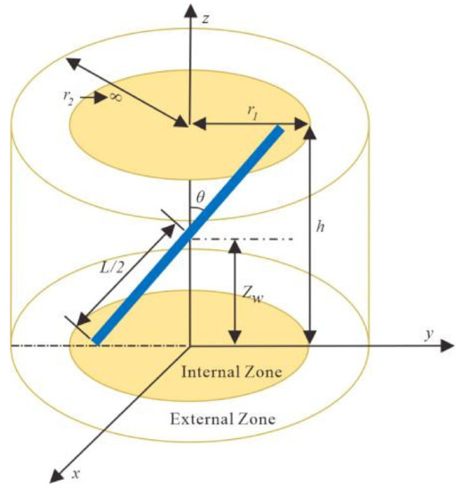
Figure 1.
Schematic diagram of the physical model.
- (1)
- The gas reservoir has an impermeable top and bottom. re represents gas reservoir radius. h represents Stratum thickness;
- (2)
- The reservoir is divided into an internal zone and external zone. r1 represents internal zone. mi represents the simulated initial formation pressure;
- (3)
- The inclined wells penetrate the entire gas reservoir. θ represents well angle. L represents well length. qsc represents constant ground production.
- (4)
- There is not an extra pressure drop or isothermal flow at the interface of the internal and external zone. The fluid is a single-phase micro-compressible fluid, ignoring gravity and capillary force.
- (5)
- Considering the anisotropy of the well bore storage coefficient, skin factor and permeability. Knhi represents the initial horizontal permeability of the gas reservoir. Knvi represents vertical initial permeability (n = 1,2, where 1 represents the internal zone, 2 represents the external zone, h represents the horizontal direction, and v represents the vertical direction);
- (6)
- The fluid conforms to Darcy’s law in the internal zone. The fluid considers non-Darcy flow and reservoir stress sensitivity in the external zone.
2.2. Equation of Motion
Low-permeability gas reservoirs have low permeability and high irreducible water saturation. The gas has an obvious non-Darcy flow when the gas adsorption is enhanced and the boundary layer appears on the pore walls, and the gas source pressure is low. The nonlinear flow model of a low-permeability gas reservoir is shown in Figure 2. δ represents the surface boundary layer thickness. r0 represents the capillary radius. v represents the flow rate through the core. ζ* represents the minimum threshold pressure gradient. ζ represents the pseudo threshold pressure gradient. p represents the pressure gradient. The relationship between the fluid flow velocity and pressure gradient in low-permeability reservoirs is shown in Figure 2b. The composition relationship curve of nonlinear segment ζ*α and quasi-linear segment αβ. α represents the critical point. η represents the pressure gradient corresponding to the critical point. β represents the end point of flow curve.
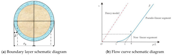
Figure 2.
Non-linear flow model schematic diagram.
Predecessors explained how non-Darcy flow is caused on a microscopic viewpoint and modified the Hagen-Poisseuille equation which considers the influence of shear stress and boundary layer thickness [26]:
where K represents the core permeability; τ0 represents the fluid yield stress; δ/r0 represents the boundary layer influence; and 8τ0/3r0 represents the fluid yield stress influence.
Equation (1) can be simplified through microscopic experiments to fit the deformation. We establish the macroscopic continuous nonlinear flow motion equation:
where c1 and c2 represent parameters obtained through experimental fitting, MPa/m.
In order to enhance the continuous nonlinear adjustment flexibility flow motion equation, we let a = −1c2/c1, b = c1−1, then Formula (2) is simplified as:
where a represents a non-linear parameter, reflecting fluid yield stress and boundary layer on flow influence. b represents the reciprocal of the threshold pressure gradient, m/MPa.
In Equation (3), when 0 < a < 1, considering the nonlinear section influence and a minimum threshold pressure gradient greater than 0, the flow curve does not pass through the origin; in this type ζ* = (1 − a)/b, b = ζ−1, which means ζ* = (1 − a) ζ. When a ≥ 1, considering the effect of nonlinear section, and the minimum threshold pressure gradient is 0, the flow curve passes through the origin; in this type b = ζ−1. When a = 0, without considering the non-linear section, the model degenerates into a pseudo threshold pressure gradient form and only considers the threshold pressure gradient influence, in this type ζ* = ζ = b−1.
Low-permeability reservoirs have strong stress sensitivity. As mining progresses, the effective stress of the rock continues to increase and the permeability continues to decrease. PEDROSA OA [27] defines permeability modulus in order to describe the relationship between permeability and pressure:
Integrating Equation (4) to get:
where Ki represents initial reservoir permeability, µm2; γ represents permeability modulus, MPa−1; and pi represents original formation pressure, MPa.
In summary, the equation of motion considering conditions such as stress sensitivity and low-permeability gas reservoir non-Darcy flow is:
2.3. Mathematical Model
2.3.1. Model Building
Based on the physical model assumptions, we combine the non-Darcy equation of motion, mass conservation equation and state equation and introduce the pseudo-pressure function to obtain the dimensionless differential equation of a low-permeability compound gas reservoir inclined well non-Darcy flow:
where the subscripts n = 1,2 represent internal and external; l = x,y,z represent directional variable; subscript D represents dimensionless; mnD represents dimensionless internal and external zone pressure; xD, yD, zD represent dimensionless direction coordinates; tD represents dimensionless time; rD, r1D represent dimensionless flow radius and internal zone radius; γmD represents dimensionless permeability modulus defined by pseudo pressure; η1,2 represents the ratio of the conduction coefficient of the internal and external zone; and λmlD represents dimensionless non-linear flow intermediate variable.
Model constraints: if , then , otherwise .
The initial condition is:
The boundary condition in the fixed production is:
The top and bottom closed external boundary condition is:
where zwD represents the longitudinal depth of the center of the inclined well of dimension one, and εD represents the micro variables of dimension one.
The boundary condition of the horizontal closed external zone boundary is:
where reD represents the maximum boundary radius of dimension one.
The external zone boundary condition of the horizontal constant pressure is:
The interface connection condition is:
where bmlD represents the dimensionless pseudo threshold pressure gradient reciprocal; zwD represents the dimensionless inclined well center longitudinal depth; εD represents dimensionless variables; reD represents dimensionless maximum boundary radius; and M1,2 represents the ratio of the internal zone and external zone.
Dimension one is defined as follows:
where mi represents reservoir initial pseudo pressure, MPa2/(mPa·s). mn represents internal and external zone pseudo pressure, MPa2/(mPa·s). T represents absolute temperature, K. qsc represents ground yield, 104 m3/d. Knhi represents initial horizontal permeability of internal and external zone, µm2. Knvi represents initial vertical permeability of internal and internal and external zone, µm2. rw, r1, re represent well bore radius, internal zone radius and boundary radius, m. t represents production time. φn represents porosity of internal and external zone, %. µn represents gas viscosity of internal and external zone, mPa.s. Ctn represents comprehensive compression coefficient of internal and external zone, MPa−1. h represents reservoir thickness, m. zw, ε represent longitudinal depth and micro variables in the center of the inclined shaft, m. γm represents Permeability modulus defined by pseudo pressure, mPa·s/MPa2. bml represents threshold pressure gradient reciprocal, mPa·s·m/MPa2.
2.3.2. Model Solving
The nonlinear flow mathematical model analytical solution is more complicated, and the author uses the finite element method to solve it. Using Galerkin’s method to obtain the finite element equation of the external zone when there is no source-sink term is:
where Ni represents the components of shape function, i = 1,2, …, n.
The internal element and the external boundary element finite element equations with closed conditions are obtained by partial integration through Green’s formula:
Transform the finite element equation into a matrix form:
where:
Further simplify the finite element equation matrix form:
where represents nonlinear coefficient matrix, represents element load vector. Superscript represents time variable.
For Equation (19) , the expression is as follows:
Equation (19) represents the balance equation of the finite element; the element in the external zone of the model can also be obtained by the same method.
Although the infinite diversion model is more in line with the measured pressure distribution of the inclined well, it is difficult to solve it. Usually, the equivalent pressure point of the uniform line source model is selected to study the inclined well pressure distribution. Cinco et al. [28] and Ozkan et al. [29] conducted a lot of research on the equivalent pressure point of deviated wells. The author used the method proposed by Cinco et al. to study the bottom hole pressure. The bottom hole equivalent pressure point value is:
where . L represents the inclined well length, m. θ represents the well angle, °. .
The Delta function can be used to obtain the line source/sink formula related to the well position. The node of the inclined well is considered as the source and sink term of the unit, and the integration of the well node are not dimensioned. The final source and sink term of the unit is limited. The element equation is:
The numerical pressure solution obtained by the finite element method can be used to consider the influence of well storage and skin coefficient through the Duhamel principle after Laplace transformation:
where S represents the skin factor; s represents the Laplace variable; CD represents the well bore storage factor.
Using the Stehfest numerical inversion, the inclined well bottom hole pressure, considering the well bore reservoir effect and the skin factor, is solved as:
3. Analysis of Flow Law
3.1. Comparison of Flow Patterns
Based on the above method, the author used Matlab programming to solve the model, draw the pseudo pressure dynamic curve of model and compare it with the Darcy flow model and pseudo threshold pressure gradient model [2]. The nonlinear flow model considers the nonlinear characteristics and the threshold pressure gradient at the same time: CD = 100, S = 1, hD = 200, θ = 60°, r1D = 15, η1,2 = 0.2, γmD = 0. The non-Darcy flow model considers both nonlinear flow and the threshold pressure gradient, a = 0.5, bmlD = 100. The pseudo threshold pressure gradient model only considers the threshold pressure gradient, a = 0, bmlD = 100; the dimensionless pseudo threshold pressure gradient of the two models is 0.01 for both.
As shown in Figure 3, 7 flow stages are divided according to the pseudo pressure dynamic curve characteristics: (1) In the well bore storage section, the pseudo pressure and its derivative curve is a coincident straight line with a slope of 1. (2) In the transition section of the skin effect, the pseudo-pressure derivative curve is hump-shaped. (3) It is mainly controlled by the well inclination angle, and gradually shows the flow characteristics of a horizontal well with the increase of the well inclination angle. When the inclination angle is greater than 60°, the early vertical radial flow and the mid-stage linear flow gradually appear. The derivative curve shows two types: a horizontal straight line and a straight line with a slope of 0.5. (4) Internal zone pseudo-radial flow, the pseudo-pressure derivative curve is a horizontal straight line with a value of 0.5. (5) Internal-external zone pseudo radial flow transition section, the slope of the pseudo pressure derivative curve is related to the ratio of the conduction coefficient of the internal and external zone. (6) External zone pseudo radial flow transition section radial flow, regardless of factors such as non-Darcy flow and stress sensitivity, the pseudo pressure derivative curve is a horizontal straight line. The position of the horizontal line is related to the pressure coefficient ratio of the internal and external zones. The larger the pressure conductivity ratio, the higher the position of the horizontal line. (7) At the boundary influence stage, different external boundary conditions have different effects on the quasi pressure and its derivative curve shape. Under closed outer boundary conditions, the pseudo pressure and its derivative curve are severely warped due to the influence of the closed boundary.
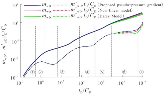
Figure 3.
Comparison of dynamic pseudo pressure curves of different models.
The model only considers the low-permeability characteristics of the external zone. The pseudo pressure and its derivative curves of the pseudo threshold pressure gradient model and the nonlinear flow model are all upturned from the pseudo radial flow section in the external zone. The magnitude of upturn of the nonlinear flow model is significantly lower than that of the pseudo threshold pressure gradient model. In order to finely characterize the low-permeability reservoir flow characteristics, the nonlinear flow section influence mechanism needs to be further researched. As the pressure gradient increases, the stagnant layer thickness gradually decreases. At this time, nonlinear flow characteristics appear.
3.2. Sensitivity Analysis
Predecessors conducted a sensitivity analysis of the nonlinear parameter a, the inclination angle θ, the radius of the internal zone r1D, and the ratio η1,2 of the internal and external zone pressure coefficient [30,31,32].
3.2.1. Non-Linear Parameters
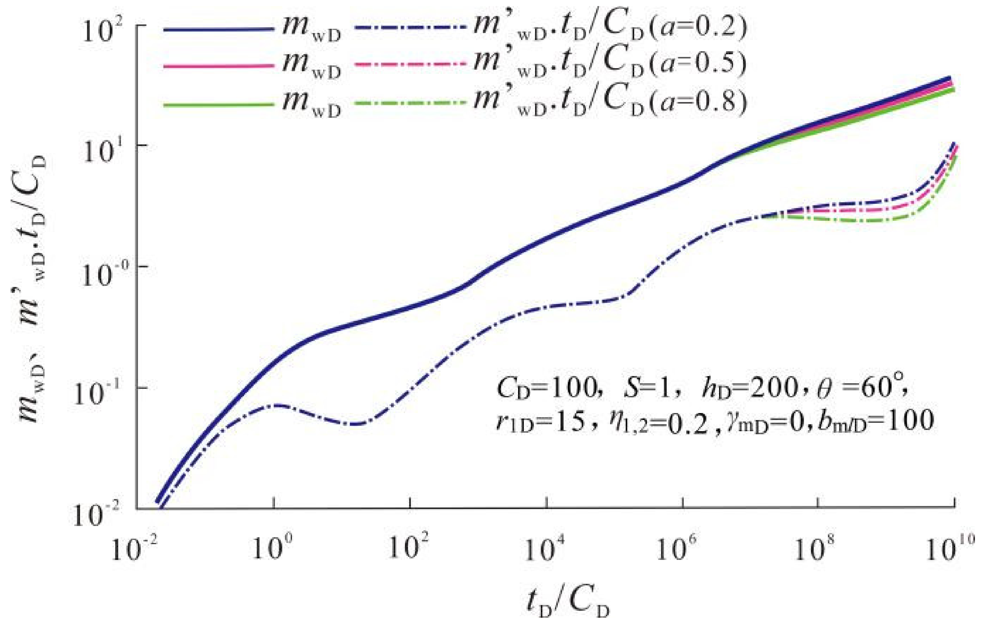
The influence of the nonlinear parameter a on the pseudo pressure dynamic curve is shown in Figure 4. As shown in Figure 4, under nonlinear flow and pseudo threshold pressure gradient influence, the pseudo pressure dynamic curve is warped in the radial flow section of the external zone. The reason is that the worse the reservoir physical properties, the greater the nonlinear flow intensity and the greater the pressure difference required for gas flow. Set the value of the dimensionless pseudo threshold pressure gradient to 0.01, and a change in nonlinear parameter a (0 < a < 1) can be found: as the value of a increases, the slope of the nonlinear section decreases, the minimum threshold pressure gradient gradually tends to 0, the additional flow resistance brought by the nonlinear flow decreases, and the curve appears in the external zone. The upward warping time of the radial flow segment is delayed, and the upward warping amplitude is reduced. Non-linear parameters have an obvious impact on the production performance of low-permeability reservoirs. It is difficult to objectively describe the dynamic characteristics of reservoir pressure when ignoring the Darcy or pseudo threshold pressure gradient model in the nonlinear flow section.
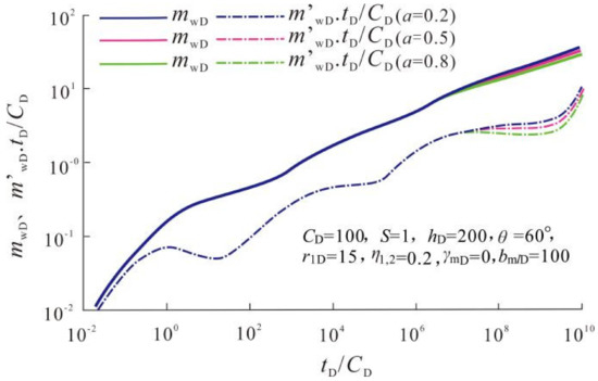
Figure 4.
Effect of the nonlinear parameter on dynamic pseudo pressure curves.
3.2.2. Well Angle
The influence of the inclination angle θ on the pseudo pressure dynamic curve is shown in Figure 5. In the control section of the inclination angle, the pressure wave has not spread far, and the inclination angle has a more obvious influence on the dynamic curve. When the inclination angle is low, the pressure dynamic curve is similar to a vertical well. As the inclination angle increases, the pressure dynamic curve gradually assumes the characteristics of a horizontal well. When the inclination angle is greater than 60°, due to the large contact area between the inclined well section and the formation, the early vertical radial flow and the mid-term linear flow gradually appear, and the pseudo pressure derivative curves show a horizontal line and a straight line with a slope of 0.5. As the inclination angle increases, the length L of the well increases, and the longer the duration of the early radial flow is. The production will be evenly distributed during the fixed production, the bottom hole pressure will decrease, and the pseudo pressure and its derivative curve will move downward. When the reservoir stress sensitivity and non-Darcy flow are not considered, the pseudo radial flow sections of the internal and external zones converge into a straight line.
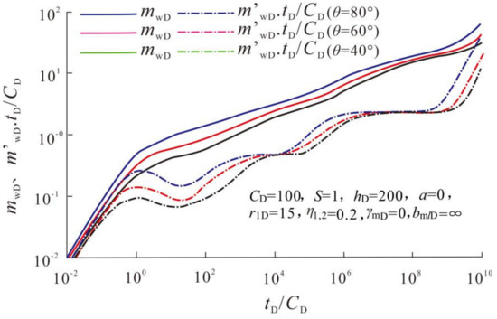
Figure 5.
Effect of the well angle on dynamic pseudo pressure curves.
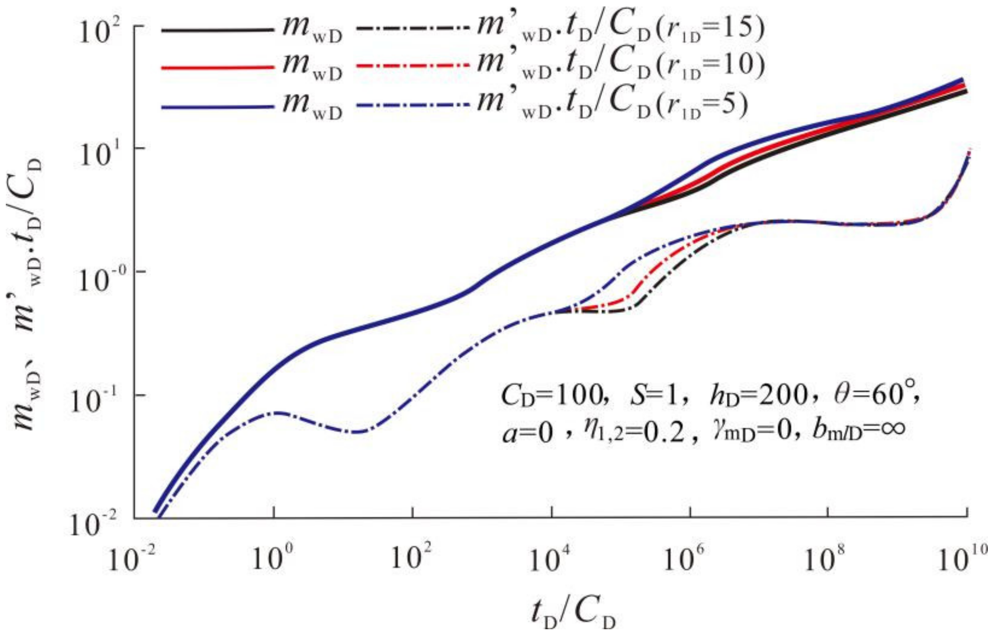
3.2.3. Internal Zone Radius
The influence of the internal zone radius on the pseudo-pressure dynamic curve is shown in Figure 6. It can be seen from Figure 6 that the internal radius affects the duration of the quasi-radial flow in the internal region and the starting time of the transition phase of the quasi radial flow in the internal and external regions. The smaller the radius of the internal zone, the shorter the duration of the pseudo-radial flow in the internal zone, and the earlier the transition phase appears. When the radius of the internal zone is small to a certain extent, the pressure wave quickly propagates to the internal boundary, and the internal boundary is not reflected in the curve. The curve cannot reflect the characteristics of the quasi radial flow in the internal zone.

Figure 6.
Effect of the internal radius on dynamic pseudo pressure curves.
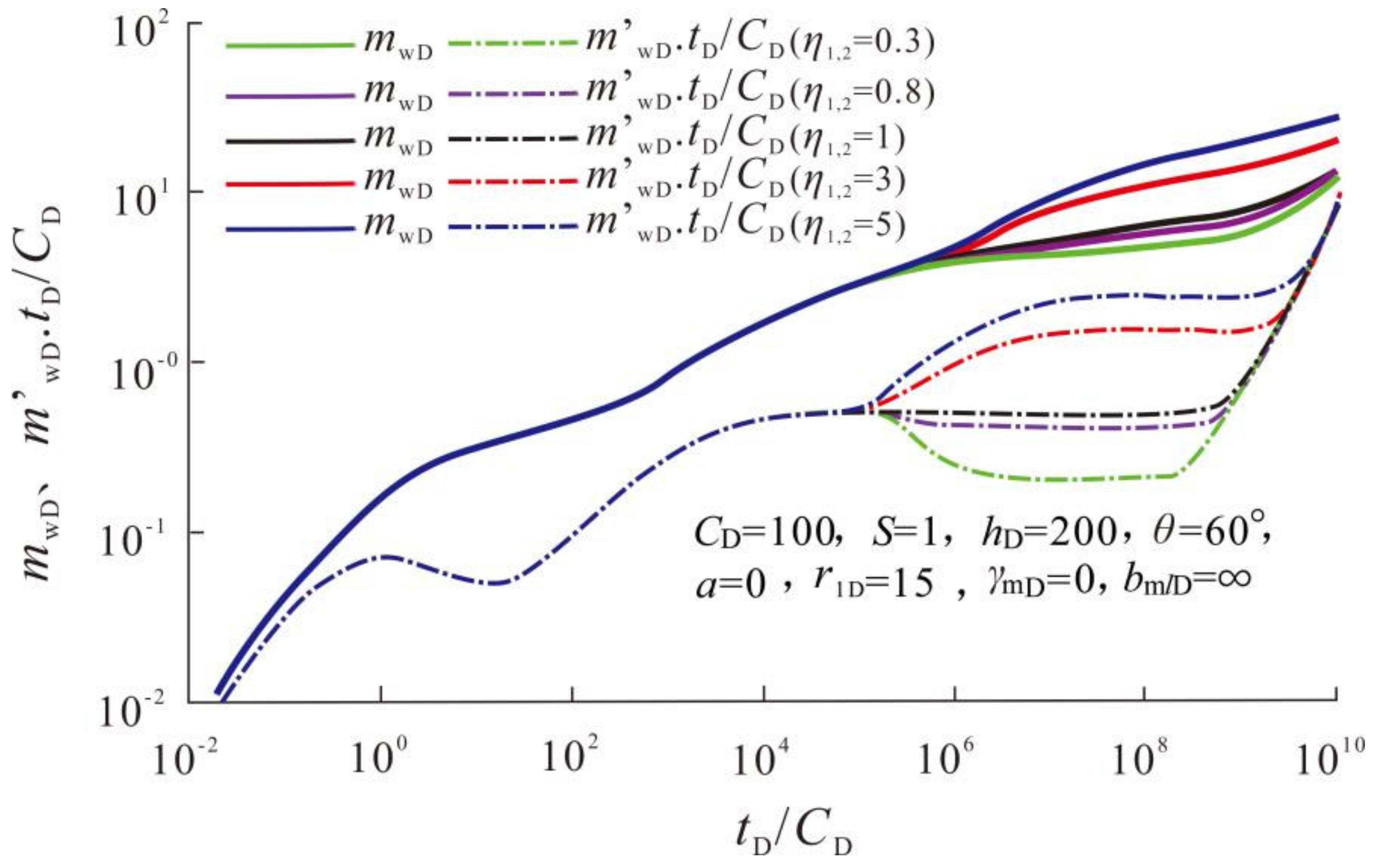
3.2.4. Internal and External Zone Pressure Coefficient Ratio
The influence of the ratio of the conduction coefficients of the internal and external zones on the pseudo-pressure dynamic curve is shown in Figure 7. The pressure conduction coefficient ratio mainly affects the slope of the pseudo radial flow transition section of the internal and external zones. When the pressure conduction coefficient of the internal and external zones is less than 1, the permeability of the external zone is better than that of the internal zone, and the pseudo radial flow transition section of the internal and external zones is concave. When the pressure conduction coefficient of the internal and external zones is greater than 1, the internal zone permeability is better than the external zone permeability, and the pseudo pressure derivative curve of the transition section is convex upwards. On the whole, as the ratio of pressure conduction coefficients in the internal and external zones increases, the flow capacity of the external zone gradually becomes worse, the flow resistance increases relatively, and the slope of the pseudo radial flow transition section in the internal and external zones gradually increases. The pseudo pressure and its derivative curve position in the flow phase are also higher.
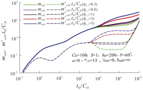
Figure 7.
Effect of the pressure conduction coefficient ratio on dynamic pseudo-pressure curves.
4. Application Case Analysis
The pressure measurement data of Well A2 in the XH gas field in the East China Sea showed obvious flow characteristics of the inclined well in the low-permeability composite gas reservoir (Figure 8). The conventional well test model and the new model were used to interpret Well A2 from Figure 8. The non-Darcy flow model for low-permeability composite gas reservoirs comprehensively considers the low-permeability characteristics of the reservoir and finely depicts the flow characteristics of each flow section. The model has a better fit with the measured pressure data and adds nonlinear coefficients, threshold pressure gradients, etc. The constraints of parameters on the fitting results effectively solve the problem of the strong diversification of reservoir parameters, as shown in Figure 8. The basic parameters and well test interpretation results of Well A2 are shown in Table 1.
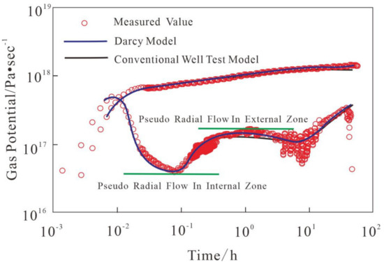
Figure 8.
Dynamic pressure fitting curves of the actual example.

Table 1.
Basic parameters and well test interpretation results of well A2.
Analyzing the pressure dynamic curve of Well A2, it can be found that the well has a small inclination angle and no early radial flow section, which is similar to the flow characteristics of a vertical well. The pressure and its derivative curve rise sharply in the later stage of flow when the pressure propagates to the fault boundary. The consideration of nonlinear flow and reservoir stress sensitivity in low-permeability gas reservoirs improves the dynamic pressure fitting effect of pseudo-radial flow outside the well. The new non-Darcy flow model explained that the permeability of the external zone was 5.9 × 10⁻³ μm2 and the skin coefficient was 8.3, while the conventional well test model explained that the permeability of the external zone was 2.5 × 10⁻³ μm2 and the skin coefficient was 7.9.
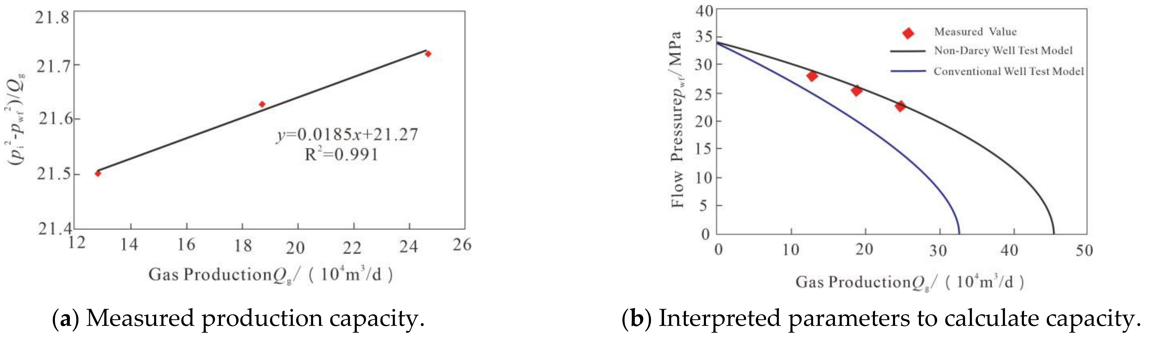
The open flow rate of this well is calculated based on the measured data of the productivity test using the binomial productivity equation to calculate the open flow rate of 47.85 × 10⁴ m3/d. The open flow rate calculated based on the parameters explained by the conventional well test model and the new non-Darcy flow model is 32.49 × 10⁴ m3/d and 45.44 × 10⁴ m3/d, respectively. As shown in Figure 9, the parameters interpreted by the new non-Darcy flow model are closer to the actual reservoir. The conventional well test model that ignores the permeability characteristics of low-permeability gas reservoirs has a large deviation between the interpretation of permeability and the actual effective permeability of the gas reservoir, which restricts the evaluation of the productivity of low-permeability reservoirs. The establishment and application of the non-Darcy well test model can effectively improve low permeability. The composite gas reservoir parameter interpretation accuracy is of great significance to the pressure and productivity evaluation of such gas reservoirs.

Figure 9.
Comparison and verification of model interpretation results.
5. Conclusions
- (1)
- Based on the microscopic mechanism of non-Darcy flow and stress sensitivity in low-permeability gas reservoirs, the flow motion equation was improved, and a non-Darcy flow mathematical model was established in low-permeability composite gas reservoir inclined wells. This was carried out using the equivalent pressure point to deal with the inner boundary conditions, and the finite element method to solve the bottom hole pressure.
- (2)
- In this paper, the bottom hole pressure dynamic curves of different models are drawn and compared. According to the curve characteristics, seven flow stages are divided, which are as follows: well bore reservoir, excessive skin effect, well inclination angle control, pseudo-radial flow in inner zone, excessive pseudo-radial flow in internal and external zone, pseudo-radial flow in external zone and boundary influence stage.
- (3)
- When the nonlinear factor increases, the pseudo-pressure dynamic curve increases upward in the pseudo-radial flow stage in the external region. When the well inclination is greater than 60°, the early vertical radial flow section gradually appears, and the duration is prolonged with the increase of the well inclination. The radius of the internal zone increases, and the duration of the quasi-radial flow phase in the internal zone is prolonged. When the pressure coefficient ratio of the internal and external zones is greater than 1.0, the slope of the transition section is positive and increases with the increase in the pressure conductivity ratio.
- (4)
- Compared with the traditional well test model, the low-permeability composite gas reservoir non-Darcy flow model fits better with the pressure dynamic curve. The main reason is to increase the constraints on the interpretation results, such as nonlinear factors, and reduce the multi-solution of the parameters. The permeability explained by the two models is significantly different, and the non-Darcy flow model reasonably evaluates low-permeability gas reservoir productivity.
Author Contributions
Conceptualization, H.L.; Formal analysis, H.L.; Validation, H.L.; Visualization, H.L.; Writing-original draft, H.L.; Writing-review and editing, H.L.; Funding acquisition, Q.Z.; Project administration, K.W.; Data curation, Y.Z. (Yuan Zeng); Software, Y.Z. (Yuan Zeng); Resources, Y.Z. (Yushuang Zhu); Supervision, Y.Z. (Yushuang Zhu); Methodology, Y.Z. (Yushuang Zhu). All authors have read and agreed to the published version of the manuscript.
Funding
This research was funded by [Yushuang Zhu] grant number [2017ZX05008-004-004-001 and 41972129] and the APC was funded by [Yushuang Zhu].
Institutional Review Board Statement
Not applicable.
Informed Consent Statement
Not applicable.
Data Availability Statement
This paper has no related reports and excludes this claim.
Conflicts of Interest
The authors declare no conflict of interest.
References
- Wei, X.; Qun, L.; Shusheng, G.; Zhiming, H.; Hui, X. Pseudo threshold pressure gradient to flow for low per- meability reservoirs. Pet. Explor. Dev. 2009, 36, 232–236. [Google Scholar] [CrossRef]
- Li, D.; Zha, W.; Liu, S.; Wang, L.; Lu, D. Pressure transient analysis of low permeability reservoir with pseudo threshold pressure gradient. J. Pet. Sci. Eng. 2016, 147, 308–316. [Google Scholar] [CrossRef]
- Zeng, B.; Cheng, L.; Li, C. Low velocity non-linear flow in ultra-low permeability reservoir. J. Pet. Sci. Eng. 2011, 80, 1–6. [Google Scholar] [CrossRef]
- Guo, J.; Zhang, S.; Zhang, L.; Qing, H.; Liu, Q. Well Testing Analysis for Horizontal Well With Consideration of Threshold Pressure Gradient in Tight Gas Reservoirs. J. Hydrodyn. 2012, 24, 561–568. [Google Scholar] [CrossRef]
- Wu, Z.; Cui, C.; Lv, G.; Bing, S.; Cao, G. A multi-linear transient pressure model for multistage fractured horizontal well in tight oil reservoirs with considering threshold pressure gradient and stress sensitivity. J. Pet. Sci. Eng. 2019, 172, 839–854. [Google Scholar] [CrossRef]
- Sun, Z.; Yang, X.; Jin, Y.; Shi, S.; Wu, M. Analysis of Pressure and Production Transient Characteristics of Composite Reservoir with Moving Boundary. Energies 2020, 13, 34. [Google Scholar] [CrossRef] [Green Version]
- Li, J.; Zhao, G.; Jia, X.; Yuan, W. Integrated study of gas condensate reservoir characterization through pressure transient analysis. J. Nat. Gas Sci. Eng. 2017, 46, 160–171. [Google Scholar] [CrossRef] [Green Version]
- Zhang, R.; Zhang, L.; Wang, R.; Zhao, Y.; Zhang, D. Research on transient flow theory of a multiple fractured horizontal well in a composite shale gas reservoir based on the finite-element method. J. Nat. Gas Sci. Eng. 2016, 33, 587–598. [Google Scholar] [CrossRef]
- Zeng, H.; Fan, D.; Yao, J.; Sun, H. Pressure and rate transient analysis of composite shale gas reservoirs considering multiple mechanisms. J. Nat. Gas Sci. Eng. 2015, 27, 914–925. [Google Scholar] [CrossRef]
- Meng, F.; Lei, Q.; He, D.; Yan, H.; Jia, A.; Deng, H.; Xu, W. Production performance analysis for deviated wells in composite carbonate gas reservoirs. J. Nat. Gas Sci. Eng. 2018, 56, 333–343. [Google Scholar] [CrossRef]
- Nie, R.; Fan, X.; Li, M.; Chen, Z.; Deng, Q.; Lu, C.; Zhou, Z.; Jiang, D.; Zhan, J. Modeling transient flow behavior with the high velocity non-Darcy effect in composite naturally fractured-homogeneous gas reservoirs. J. Nat. Gas Sci. Eng. 2021, 96, 104269. [Google Scholar] [CrossRef]
- Gao, Y.; Rahman, M.M.; Lu, J. Novel Mathematical Model for Transient Pressure Analysis of Multifractured Horizontal Wells in Naturally Fractured Oil Reservoirs. ACS Omega 2021, 6, 15205–15221. [Google Scholar] [CrossRef]
- Jiang, R.; Zhang, F.; Cui, Y.; Qiao, X.; Zhang, C. Production performance analysis of fractured vertical wells with SRV in triple media gas reservoirs using elliptical flow. J. Nat. Gas Sci. Eng. 2019, 68, 102925. [Google Scholar] [CrossRef]
- Xu, Y.; Liu, Q.; Li, X.; Meng, Z.; Yang, S.; Tan, X. Pressure transient and Blasingame production decline analysis of hydraulic fractured well with induced fractures in composite shale gas reservoirs. J. Nat. Gas Sci. Eng. 2021, 94, 104058. [Google Scholar] [CrossRef]
- Dongyan, F.; Jun, Y.; Hai, S.; Hui, Z.; Wei, W. A composite model of hydraulic fractured horizontal well with stimulated reservoir volume in tight oil & gas reservoir. J. Nat. Gas Sci. Eng. 2015, 24, 115–123. [Google Scholar]
- Wu, M.; Ding, M.; Yao, J.; Xu, S.; Li, L.; Li, X. Pressure transient analysis of multiple fractured horizontal well in composite shale gas reservoirs by boundary element method. J. Pet. Sci. Eng. 2018, 162, 84–101. [Google Scholar] [CrossRef]
- Zhang, Q.; Zhang, L.; Liu, Q.; Jiang, Y. Pressure Performance of Highly Deviated Well in Low Permeability Carbonate Gas Reservoir Using a Composite Model. Energies 2020, 13, 5952. [Google Scholar] [CrossRef]
- Cao, R.; Wang, Y.; Cheng, L.; Ma, Y.Z.; Tian, X.; An, N. A New Model for Determining the Effective Permeability of Tight Formation. Transp. Porous Media 2016, 112, 21–37. [Google Scholar] [CrossRef] [Green Version]
- Wu, J.; Cheng, L.; Li, C.; Cao, R.; Chen, C.; Cao, M.; Xu, Z. Experimental Study of Nonlinear Flow in Micropores Under Low Pressure Gradient. Transp. Porous Media 2017, 119, 247–265. [Google Scholar] [CrossRef]
- Karimpouli, S.; Tahmasebi, P. A Hierarchical Sampling for Capturing Permeability Trend in Rock Physics. Transp. Porous Media 2017, 116, 1057–1072. [Google Scholar] [CrossRef]
- Albinali, A.; Holy, R.; Sarak, H.; Ozkan, E. Modeling of 1D Anomalous Diffusion in Fractured Nanoporous Media. Oil Gas Sci. Technol.—Rev. D’ifp Energies Nouv. 2016, 71, 56. [Google Scholar] [CrossRef] [Green Version]
- Wang, H.; Wang, J.; Wang, X.; Chan, A. Multi-Scale Insights on the Threshold Pressure Gradient in Low-Permeability Porous Media. Symmetry 2020, 12, 364. [Google Scholar] [CrossRef] [Green Version]
- Luo, L.; Cheng, S. In-situ characterization of nonlinear flow behavior of fluid in ultra-low permeability oil reservoirs. J. Pet. Sci. Eng. 2021, 203, 108573. [Google Scholar] [CrossRef]
- Carpio, R.R.; DAvila, T.C.; Taira, D.P.; Ribeiro, L.D.; Viera, B.F.; Teixeira, A.F.; Campos, M.M.; Secchi, A.R. Short-term oil production global optimization with operational constraints: A comparative study of nonlinear and piecewise linear formulations. J. Pet. Sci. Eng. 2021, 198, 108141. [Google Scholar] [CrossRef]
- Jiang, R.Z.; Li, L.K.; Xu, J.C.; Yang, R.F.; Zhuang, Y. A nonlinear mathematical model for low-permeability reservoirs and well-testing analysis. Acta Pet. Sin. 2012, 33, 264–268. [Google Scholar]
- Xu, J.C.; Sun, B.J.; Chen, B.L. A hybrid embedded discrete fracture model for simulating tight porous media with complex fracture systems. J. Pet. Sci. Eng. 2019, 174, 131–143. [Google Scholar] [CrossRef]
- Pedrosa, O.A. Pressure transient response in stress-sensitive formations. In SPE California Regional Meeting; OnePetro: Richardson, TX, USA, 1986. [Google Scholar]
- Cinco, L.H.; Miller, F.G. Unsteady-state pressure distribution created by a directionally drilled. J. Pet. Technol. 1975, 27, 1392–1400. [Google Scholar] [CrossRef]
- Ozkan, E.; Raghavan, R.A. Computationally efficient transient-pressure solution for inclined wells. SPE Reserv. Eval. Eng. 2000, 3, 414–425. [Google Scholar] [CrossRef]
- Ezulike, O.; Igbokoyi, A. Horizontal well pressure transient analysis in anisotropic composite reservoirs-A three dimensional semi-analytical approach. J. Pet. Sci. Eng. 2012, 96, 120–139. [Google Scholar] [CrossRef]
- Wei, Z.; Ruizhong, J.; Jianchun, X.; Yihua, G.; Yibo, Y. Production performance analysis for horizontal wells in composite coal bed methane reservoir. Energy Explor. Exploit. 2017, 35, 194–217. [Google Scholar] [CrossRef] [Green Version]
- Fan, D.Y.; Zeng, H.; Jun, Y.; Zhao, J.; Niu, N. Analytical method of the unstable well test in tight oil reservoirs considering the starting pressure gradient. J. Northeast Pet. Univ. 2021, 45, 102–112. [Google Scholar]


Publisher’s Note: MDPI stays neutral with regard to jurisdictional claims in published maps and institutional affiliations. |
© 2022 by the authors. Licensee MDPI, Basel, Switzerland. This article is an open access article distributed under the terms and conditions of the Creative Commons Attribution (CC BY) license (https://creativecommons.org/licenses/by/4.0/).