Abstract
The internal energy (U-energy) conversion to free energy (F-energy) and energy dissipation (S-energy) is a basic process that enables the continuity of life on Earth. Here, we present a novel method of evaluating F-energy in a membrane system containing ternary solutions of non-electrolytes based on the version of the Kedem–Katchalsky–Peusner (K–K–P) formalism for concentration polarization conditions. The use of this formalism allows the determination of F-energy based on the production of S-energy and coefficient of the energy conversion efficiency. The K–K–P formalism requires the calculation of the Peusner coefficients and (i, j ∈ {1, 2, 3}, r = A, B), which are necessary to calculate S-energy, the degree of coupling and coefficients of energy conversion efficiency. In turn, the equations for S-energy and coefficients of energy conversion efficiency are used in the F-energy calculations. The form of the Kedem–Katchalsky–Peusner model equations, containing the Peusner coefficients and , enables the analysis of energy conversion in membrane systems and is a useful tool for studying the transport properties of membranes. We showed that osmotic pressure dependences of indicated Peusner coefficients, energy conversion efficiency coefficient, entropy and energy production are nonlinear. These nonlinearities were caused by pseudophase transitions from non-convective to convective states or vice versa. The method presented in the paper can be used to assess F-energy resources. The results can be adapted to various membrane systems used in chemical engineering, environmental engineering or medical applications. It can be used in designing new technologies as a part of process management.
1. Introduction
Energy conversion is one of the basic phenomena that ensure the continuity of life on Earth. It occurs in various types of micro- and macrosystems including membrane systems. The study of membrane transport processes is both cognitive and applicable [1,2]. Cognitive studies include molecular mechanisms of the exchange of fluids and dissolved substances by biological and/or synthetic membranes [3]. Membranes in living systems act as regulators of the transport of substances necessary for living organisms to maintain their metabolic activity, regulate the pressure balance and for structural integrity. The study of membrane transport has applications to water and wastewater technology, the food industry, biorefineries and energy-based renewable sources [4] and in medicine to drug carriers such as liposomes, nanomicelles or dendrimers [5] or active membrane dressings [6].
All processes in various types of systems, including living systems, require energy supply. In living systems, this feeding takes place through the uptake of certain nutrients, called nutrition. This applies to every living cell as well as the whole organism [1]. Food contains energy, the source of which is the sun [3]. The energy required to start and run technological processes also comes from natural sources (sun, wind, minerals, chemical reactions, nuclear reactions, etc.) However, its conversion to a useful form, due to limited resources, should be characterized by high efficiency. Evaluation of this efficiency requires specialized research tools, which include the laws of thermodynamics and thermodynamic models of transport, including membrane transport [1]. These laws and models are used to design and manage processes and systems. One of the most important elements in the energy conversion process are boiler and water-cooling systems. In these systems, membrane separation plays an essential role [2].
By this energy, we mean the chemical potential energy, which is a component of the internal energy (U). Its part called the free energy (F) is related to the internal energy by the expression F = U − TS, in which T is the absolute temperature and S is the thermodynamic entropy). The TS product is a measure of degraded energy [1,7]. F-energy is converted into physicochemical systems, including living organisms, into mechanical work related to the movements of entire systems, as well as the movements of mass and charge within them. The conversion of free energy into mechanical work can take place in a thermal, osmotic-diffusion, electrical and/or mechanical manner. They are determined by appropriate thermodynamic stimuli such as gradients: temperature (∇T), concentration (∇C), electrical potentials (∇V) and/or mechanical pressure (∇P). A specific thermodynamic stimulus can cause a specific diffusion and/or osmotic transport of a substance, heat transport, electric charge transport, etc. [7,8]. Transport against viscous forces, or dissipative forces, means conducting distributed work, and transport against external forces means useful work.
To describe transport processes in membrane systems, thermodynamic models were developed that include diffusion [9,10] and friction [11,12,13] models and models based on Onsager non-equilibrium thermodynamics [1,7,8,9], statistical physics [14,15] and network thermodynamics [16,17,18,19,20,21,22,23,24,25]. Models that use Onsager thermodynamics are based on the assumption that the dissipation function exists, which is a measure of energy dissipation [1,7,8,9]. In close-to-equilibrium systems, i.e., those in which the free energy dissipation rate is low, it can be assumed that there are linear relationships between the fluxes and the driving thermodynamic forces. The Kedem–Katchalsky (KK) formalism, developed in accordance with these principles, considers the interaction between the solvent and dissolved substances [9]. This gives a set of phenomenological membrane coefficients (Lp, σ, ω) that can be independently determined experimentally [7]. Moreover, this formalism provides a theoretical basis for the analysis of volume and solute fluxes in various membrane systems. Therefore, the KK equations belong to the group of basic research tools for membrane transport in both biological and artificial systems. Several versions of these equations are used: classic [7,9], Kargol’s [26], Cheng and Pinsky [8] and Kedem, Katchalsky and Peusner [16,17,18,19,20,21,22,23,24,25].
The idea of “network thermodynamics, NT” was independently introduced by Leonardo Peusner in 1970 [17] and Oster, Perelson and Katchalsky in 1971 [16]. The idea of Peusner’s NT is based on a combination of Onsager thermodynamics and the theory of electric circuits [27]. Peusner applied his ideas to energy conversion systems [28], membrane systems and processes [28,29], Brownian motion [30] and chemical reactions with diffusion [31]. Peusner presented the methods of transforming the linear Onsager equations with the use of hybrid descriptions [27,28,29]. Peusner also showed the ways of deriving the L, R, H and P versions of the Kedem–Katchalsky (K–K) equations by means of a series of lattice transformations and introduced the “super Q” coupling parameter.
The network form of KK equations is obtained by symmetric and/or hybrid transformation of classical KK equations using Peusner lattice thermodynamics (Peusner’s network thermodynamics, Peusner’s NT) [17,18,19,20,21,28]. For homogeneous and heterogeneous binary solutions of non-electrolytes, there are two symmetrical and two hybrid forms of the KK equations. There are two symmetrical and six hybrid forms of the network Kedem–Katchalsky–Peusner (K–K–P) equations, both for the conditions of homogeneity and concentration polarization of ternary solutions of non-electrolytes [22,23,24,25].
In this paper, we aim to calculate the amount of free energy (F-energy) that is available to perform thermodynamic work, by determining energy dissipation (S-energy). To determine energy dissipation, we propose a novel form of network K–K–P equations, , that contain the Peusner coefficients (i, j ∈ {1, 2, 3}, r = A, B) and the equation for the global source of entropy (). Additionally, we calculate novel membrane transport coefficients, and , the matrix coefficients = and = To determine the , we measure volume flux () and solute fluxes of glucose ( and/or ethanol (). The is calculated for the steady state polarization conditions and homogeneity of solutions. Moreover, we introduce an energy conversion efficiency coefficient, that is necessary to determine F-energy. Presented results that describe osmotic pressure dependences of Peusner coefficients, energy conversion efficiency coefficient and S-entropy production improve our understanding of membrane transport in concentration polarization conditions. In this study, we use a cellulose membrane; however, our method of F-energy determination can be adapted to other types of membrane systems to describe the transport of a multi-component solution through the membrane and to improve energy production properties of novel membrane systems.
2. Materials and Methods
2.1. Membrane System
The membrane is treated as a “black box” type for solvent and dissolved non-electrolyte substances. Similarly to previously published papers [22,23,24,25,26,27,28], the membrane transport was examined in a system containing non-electrolyte ternary solutions, schematically shown in Figure 1a. In this system, a membrane (M) separating the compartments (h) and (l) is isotropic, symmetrical, electrically neutral and selective for the solvent and dissolved substances. The concentrations of solutions that fill compartments (h) and (l) at the initial moment (t = 0) are defined as and ( > , k = 1, 2).
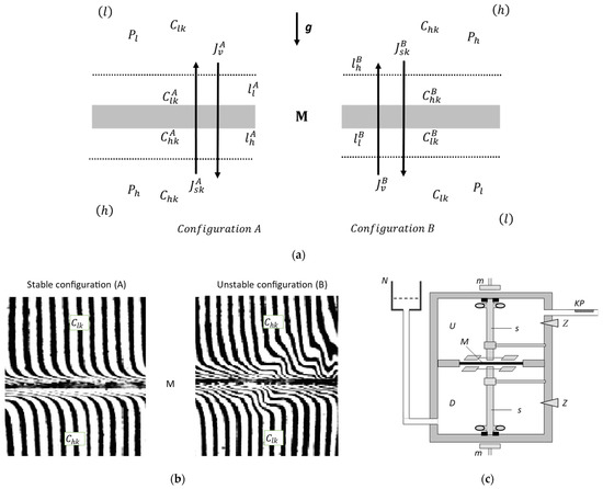
Figure 1.
(a) Schematic representation of the single-membrane system in configuration A and B. M—membrane, g—gravitational acceleration, and —the concentration boundary layers in configuration A, and —the concentration boundary layers in configuration B, and —mechanical pressures, and —global solution concentrations ( > ), , , and —local (at boundaries between membrane and CBLs) solution concentrations, and —solute and volume fluxes in configuration A, respectively, and —solute and volume fluxes in configuration B, respectively, (k = 1 or 2). (b) Interferograms for aqueous solution of glucose and ethanol for configurations A and B of a single-membrane system ( = 98.1 kPa and = 490.2 kPa), based on [32]. (c) Scheme of a measuring system (U, D—measuring vessels, N—external solution reservoir, s—mechanical stirrers, M—membrane, KP—graduated pipette, m—magnets, z—stoppers) [33].
For a membrane positioned in a horizontal plane orientation (perpendicular to the gravity vector), solutions are positioned in configurations A or B (r = A or B). In configuration A, the solution with concentration is located in the compartment above the membrane, whereas the solution with concentration is located in the compartment below the membrane. In configuration B, the orientation of the solutions relative to the membrane is reversed.
We investigated the isothermal and stationary membrane transport processes, for which we determined the volume flux () and the solute fluxes ) (k = 1, 2 and r = A, B). These fluxes can be described for ternary solutions of non-electrolytes and the conditions of concentration polarization using the KK equations [18,19,20,21,22,23,24]. Under concentration polarization conditions, molecules of dissolved substances that diffuse through the membrane create concentration boundary layers (CBLs) on both sides of the membrane. These CBLs are denoted by with thickness of and with thickness of depending on the average concentrations of (k = 1, 2) [34,35]. The creation of and causes decrease in concentration at a membrane–solution interface from to and increase from to . This means that for > 0 the following relations are fulfilled: > , > and > (k = 1, 2) [19]. The symbols and denote the densities of the solutions at the interface between /M and M/ as well as and denote the densities of the solutions outside the layers. The following relations are possible between these densities: < or > , > or < , > or < and > or < . There are relations between the densities and concentrations of the solutions = (1 + + ), where = and = (for glucose solutions in aqueous ethanol solution > 0 and < 0) [35]. If the solution with a lower density is above the membrane, then the complex /M/ loses hydrodynamic stability and gravitational (convective) instabilities are observed in the vicinity of the membrane [32,36,37].
To visualize the CBLs creation process, the Mach–Zehnder interferograms are presented for the membrane positioned in the horizontal plane that separates a solution with a concentration (water) and a solution with a concentration containing water, glucose, 40 mol m−3 and ethanol, 200 mol m−3 (Figure 1b) [32]. It should be noted that when there is clean water on both sides of the membrane, there is no CBL formation as the interference fringes are parallel to each other, rectilinear and perpendicular to the surface of the membrane. The bending of the interference fringes in the near-membrane regions is indicative of the formation of CBLs. In the stable configuration (A), the thickness of these layers increases with time. In the unstable configuration (B), the thickness of CBLs does not increase with time, but oscillates in the range of 300–400 µm [32]. These oscillations are due to the combined presence of glucose and ethanol diffusion transport and natural (gravitational) convection. Diffusive transport leads to CBL’s co-creation, and free convection causes their destruction. The evidence for the existence of natural convection is the deformation of the interference fringes.
The measure of concentration polarization is the coefficient of concentration polarization () that depends both on the concentration of the solutions separated by the membrane and the configuration of the membrane system (r = A, B). In special cases, when the thicknesses and fulfill the conditions = = and = = , then the value of the coefficient satisfies the condition = = [32,34,35,36,37,38].
2.2. Methodology for Measuring the Osmotic and Solute Fluxes
The study of osmotic volume and solute fluxes was carried out using the measuring set described in the previous paper [33] and presented in Figure 1c. The set consists of two cylindrical measuring vessels with a volume of 200 cm3 each. One vessel (U) contained a ternary aqueous glucose and ethanol solution. The second vessel (D) contained an aqueous solution of glucose and ethanol with a constant concentration = = 1 mol m−3. The Nephrophan membrane (Orwo VEB Filmfabrik, Wolfen, Germany) with an area A = 3.36 cm2 was located in a horizontal plane and separated two aqueous glucose (subscript 1) and ethanol (subscript 2) solutions with concentration = 1–71 mol m−3, and = 201 mol m−3. Therefore, the difference in osmotic pressures of aqueous glucose solutions () was in the range 0–171.6 kPa. The difference in ethanol osmotic pressures () was constant and equal to 490.2 kPa. The transport properties of this membrane were determined by following parameters: hydraulic permeability (), reflection (σ) and diffusion permeability (ω) [7]. The values of these coefficients for glucose (subscript 1) and ethanol (subscript 2) were: = 4.9 × 10⁻¹² m3 N−1 s−1, = 0.068, = 0.025, = 0.8 × 10⁻⁹ mol N−1 s−1, = 0.81 × 10⁻¹³ mol N−1 s−1, = 1.43 × 10⁻⁹ mol N−1 s−1 and = 1.63 × 10⁻¹² mol N−1 s−1 [36].
An appropriately graduated pipette (KP) was positioned parallel to the plane of the membrane and connected to the vessel containing the higher concentration of the solution (U) to measure the volume change () of the solution in this vessel of the plumbing system. The second vessel (D) was connected to a reservoir (N) of an aqueous solution of glucose and/or ethanol with a concentration of = = 1 mol m−3, adjustable in height relative to the pipette to enable adjustment of the hydrostatic pressure () in the measuring set. The measurements were carried out according to the procedure described in [36]. The increases in were measured under stirring at 500 rpm. When a steady-state flux was achieved, stirring was turned off and the increases in were also measured until the steady state of the flux was obtained. Each experiment was performed in configuration A, in which the test solution was filled into the vessel below the membrane, and in configuration B, in which the test solution was in the vessel above the membrane. The volume flows were from the vessel with a lower concentration of solutions to the vessel with a higher concentration of solutions, and the flux of dissolved substances in the opposite direction. Therefore, it was assumed that in the configuration A the fluxes (volume flux), (solute flux), (advective flux) and the concentration differences (k = 1, 2) were negative, and in the configuration B they were positive.
The investigations were carried out in isothermal conditions for T = 295 K. The volume flux was calculated based on measurements of the volume change () in the pipette in time Δt through the membrane surface A, using the formula = () ()−1 (r = A, B). Fluxes of dissolved substances were calculated based on the formula = A−1 ()−1 (k = 1, 2; r = A, B), —volume of the measuring vessel (D), —global concentration changes in the studied solutions. was determined using 14C-glucose and 14C-ethanol for four measurement sets: (1) aqueous solution of 14C-glucose and ethanol in a configuration A, (2) aqueous solution of 14C-glucose and ethanol in a configuration B, (3) aqueous solution of 14C-ethanol and glucose in a configuration A, (4) aqueous solution of 14C-ethanol and glucose in a configuration B. Radioactivity was measured using scintillation counter [39]. Arithmetic mean was calculated of electric pulses counts in 100 timepoints and five diffusion duration times 1 h, 1.5 h, 2 h, 2.5 h or 3 h. Then, we used a calibration curve to determine for the average number of pulse counts determined for each diffusion time. Next, was determined for each 0.5 h time interval and arithmetic mean of the four was calculated.
To experimentally study the volume and solute fluxes in both configurations, we first determined the characteristics = , = and = ( = 1, 2; r = A, B) for different composition and different concentration of solutions. Each series of measurements of the above characteristics were performed in triplicate. Based on their characteristics, for the steady state, the characteristics = , ), ) and =, ) were prepared. Measurement error of the fluxes and and did not exceed 10% and the solution preparation error did not exceed 1%.
2.3. The Kr form of Kedem–Katchalsky–Peusner Equations for Non-Electrolyte Solutions in Concentration Polarization Conditions
For the conditions of homogeneity of solutions that are uniformly mechanically stirred, the volume osmotic flux () and the solute fluxes () do not depend on the configuration of the membrane system. For the conditions of the polarization of concentration solutions, the creation of CBLs and reduces to and to [36]. In polarization concentration conditions, the volume flux () and solute fluxes () depend on the configuration of the membrane system and the concentration characteristics of and are nonlinear [36,40]. These volume and solute fluxes can be described by the Kedem–Katchalsky equations for ternary solutions of non-electrolytes and the conditions of concentration polarization:
where —volume flux (m s−1), and —fluxes of dissolved substances “1” and “2” (mol m−2s−1), respectively, —hydraulic permeability coefficient, and —membrane reflection coefficients for substances “1” and “2“, respectively, and —membrane permeability coefficients for substances ”1“and ”2“ generated by osmotic pressure with indexes ”1“and ”2“, respectively, and and —solute permeability coefficients for substances ”1“ and ”2“ generated by osmotic pressures with the indices ”2“ and ”1“, respectively, —hydraulic concentration polarization coefficient, and —osmotic concentration polarization coefficients, , , and —coefficients of diffuse concentration polarization and and —coefficients of advective concentration polarization. = is the difference of hydrostatic pressures ( and means higher and lower hydrostatic pressure value), = (– ) is the difference of osmotic pressures, RT is the product of the gas constant and the absolute temperature, while and are the concentrations of the solutions, > , k = 1, 2. = (– )[ln ()]−1 ( = 1, 2) is the average concentration of solutes in the complex /M/, and —concentration boundary layers, M—membrane. The first component of the Equation (1) = is the volume hydraulic flux, while the second, ( + ) = —volume osmotic flux. The first and second components of Equations (2) and (3) are diffusion fluxes = + and = + . In turn, the third component of Equations (2) and (3) is advective flux = and = . Mathematical model that was used to determine energy conversion in the membrane system [7,17,25,41] is described in Appendix A. Equations (A1)–(A15) are used to calculate dependences shown in Figures 1–8. In Appendix A, we also include physical interpretation of membrane transport parameters (Table A1) and physical interpretation of concentration polarization coefficients (Table A2).
3. Results and Discussion
3.1. Osmotic and Hydrostatic Pressure Dependencies of , and and
Figure 2a shows the dependence of the volume flux () on the glucose osmotic pressure difference () at the constant value of the ethanol osmotic pressure difference ( = 490.2 kPa) and the constant value of the hydrostatic pressure difference ( = 0). Curves 1A and 2A are determined for configurations A and curves 1B and 2B for configuration B of a single-membrane system. Additionally, curves 1A and 1B are plotted for the homogeneity conditions, whereas curves 2A and 2B for concentration polarization conditions. For homogenous solutions, the dependencies = f(, = 490.2 kPa, = 0) (curves 1A and 1B) are linear, while for the conditions of concentration polarization (curves 2A and 2B) are nonlinear.
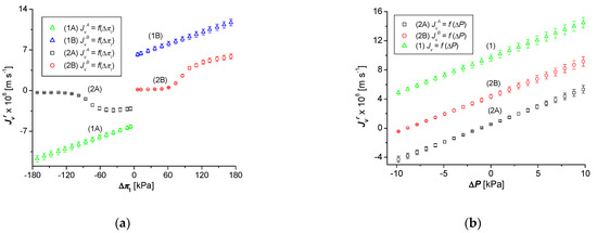
Figure 2.
Volume fluxes () as function of (a) the osmotic pressure of glucose pressure difference () with a constant osmotic pressure difference of ethanol ( = 490.2 kPa) and = 0 for stirred solutions (1A, 1B) and not stirred solutions (2A, 2B), (b) the hydrostatic pressure difference () with a constant osmotic pressure difference of both glucose ( = 96.8 kPa) and ethanol ( = 490.2 kPa) for stirred solutions (1A, 1B) and not stirred solutions (2A, 2B).
Figure 2b shows the dependences of the volume flux () for the conditions of solution homogeneity (curves 1A and 1B) and concentration polarization (curves 2A and 2B) as a function of the difference of hydrostatic pressures () at constant values of = 96.8 kPa and = 490.2 kPa for configurations A (curve 2A) and B (curve 2B) of a membrane system. This figure shows that is the sum of the volume osmotic flux () and the volume hydraulic flux ().
The dependence of the glucose diffusion flux (, r = A, B) on for constant = 0 and = 490.3 kPa, and for configurations A (curves 1A and 2A) and B (curves 1B and 2B) of the membrane system are shown in Figure 3a. For the conditions of homogeneity of solutions, the dependencies = f(, = 490.2 kPa, = 0) (curves 1A and 1B) are linear, while for the conditions of concentration polarization (curves 2A and 2B) are nonlinear.
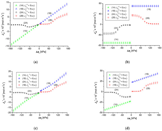
Figure 3.
Glucose flux () (a), ethanol flux () (b), advective glucose flux () (c), advective ethanol flux () (d) as functions of osmotic pressure difference of glucose () with a constant osmotic pressure of ethanol ( = 490.3 kPa) and = 0: for stirred solutions (1A, 1B), for non-stirred solutions (2A, 2B). Configuration A of the membrane system —curves 1A and 2A, configuration B—curves 1B and 2B.
Figure 3b shows the dependences of the ethanol diffusion flux (, r = A, B) on , = 490.3 kPa and = 0 for configuration A (curves 1A and 2A) and configuration B (curves 1B and 2B). For the conditions of homogeneity of the solutions, the dependences = const. (curves 1A and 1B) are linear, while for the concentration polarization conditions (curves 2A and 2B) are nonlinear. The dependence of the glucose advective flux(, r = A, B) on for the set value of = 0 and = 490.3 kPa for configurations A (curves 1A and 2A) and B (curves1B and 2B) of the membrane system are shown in Figure 3c. For the homogeneity conditions of the solutions, the dependences = f(, = 490.2 kPa, = 0) (curves 1A and 1B) are linear, while for the concentration polarization conditions (curves 2A and 2B) are nonlinear.
Figure 3d shows the dependence of the ethanol advection flux(, r = A, B) on , ( = 490.3 kPa and = 0) for configuration A (curves 1A and 2A) and configuration B (curves 1B and 2B). For the homogeneity conditions of the solutions, the relationship = f(, = 490.2 kPa, = 0) (curves 1A and 1B) are linear, while for the concentration polarization conditions (curves 2A and 2B) are nonlinear. The nonlinearity of the curves 2A and 2B shown in Figure 2a and Figure 3a–d are a consequence of the diffusive creation of CBLs or their destruction by natural convection. These processes cause nonlinear changes in the values of , and (k = 1, 2 and r = A, B) in different ranges of , depending on the configuration of the membrane system. Changing the configuration of the membrane system from A to B or vice versa in the specified ranges of causes the transition from the convective state, with a greater value of , and , to non-convection, with a lower value of , and , or vice versa. The transition from non-convective to convective, or vice versa, causes a nonlinear increase in and . Curves 2A and 2B presented in Figure 2a and Figure 3a–d show that for ≥ −108.75 kPa and for ≥ +58.8 kPa, a transition from a non-convective to a convective state is observed. In contrast, the curves 2A and 2B presented in Figure 3b show that for ≥ −58.9 kPa and for ≥ +108.8 kPa, a transition from a convective to a non-convective state is observed.
3.2. Osmotic Pressure Dependencies of , and
The coefficients , , and were calculated using the formulas listed in Table A2. Concentration polarization does not occur when the membrane separates solutions with the same concentrations ( = ). Therefore, the hydraulic fluxes are identical, = , for both homogenous and concentration polarization conditions at least for of ~105 Pa. Thus, it can be assumed with sufficient approximation that = 1.
The fluxes shown in Figure 2a and Figure 3 were substituted into these formulas to calculate the coefficients , and . The dependences = f (), = f () and = f () (k = 1, 2 and r = A, B) for = 490.3 kPa and = 0 for configurations A and B are presented in Figure 4. We observed different rates of increase in configuration B and decrease in configuration A of the coefficient values , and accompanying the growth of . For configuration A, the values of the coefficients , and are weakly dependent on the values of satisfying the following relations: −36.8 kPa ≤ ≤ 0 kPa and < −122.5 kPa. In turn, for configuration B, the appropriate relations for have the form—0 ≤ ≤ 36.8 kPa and > 134.1 kPa. For configuration A, a step change of , and occurs for assuming values in the range −122.5 kPa ≤ ≤ −73.5 kPa, while for configuration B, a step change of , and occurs for , satisfying the condition 36.8 kPa ≤ ≤ 122 kPa. It should be noted that for configuration A the value of , and increases from 0.067 to 0.47, and for configuration B the value of , and increases from 0.055 to 0.47. Changes in the values of , and are related to the jump changes in the values of , and , whereas the step changes in the values of , and are related to the transition of CBLs from a non-convective to a convective state.
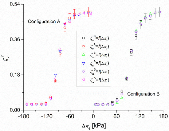
Figure 4.
Coefficients , and (k = 1, 2 and r = A, B) as functions of osmotic pressure difference of glucose () with a constant osmotic pressure of ethanol ( = 490.3 kPa) and = 0.
To analyze the stability of CBLs, gravitational convection in a membrane system characterized by a rigid membrane surface and a free CBL surface in a measurement chamber is taken into account [42,43]. The critical value of the Rayleigh number () is 1100.6 [43]. Figure 4 shows that the point with the coordinates = = ≈ 0.16, ≈ 84 kPa and ≈ 490.3 kPa can be considered as the critical point of the transition from the convection-free state or vice versa. Taking into account a previously presented [37] equation
and the following data = 9.81 m s−2, = 0.69 × 10⁻⁹ m2s−1, = 1.012 × 10⁻⁶ m2s−1, = 998 kg m−3, = 8.31 J mol−1K−1, = 295 K, = 0.8 × 10⁻⁹ mol N−1s−1, = 0.06 kg mol−1, = −0.009 kg mol−1, we obtain ≈ 1191.2. This value of is consistent with the value presented in the paper [43] with only 8% difference.
3.3. Calculations of the Coefficients , and
The values of the coefficients , , (I, j ∈ {1, 2, 3}, r = A, B) were calculated based on Equations (A1)–(A3) and (A5) for glucose in aqueous ethanol solutions. In Equations (A1)–(A3) and (A5) there are practical coefficients describing the transport properties of the membrane (, , , , , and ), the average concentrations of substances “1” and “2” in the membrane (, ) and the concentration polarization coefficients (, , , , , , , and ). The values of these coefficients were determined using the following conditions: = 1, , , = = and = = [23,24]. Dependencies = f (), = f () and = f () (k = 1, 2 and r = A, B) are shown in Figure 4.
Figure 5a shows the dependence = f(, = 490.2 kPa). For the homogeneity conditions of the solutions, the value of the coefficient is independent of and the configuration, which means that it is constant and amounts to = 0.23 × 10¹² N s m−3. This case is illustrated by the curves 1A and 1B. For the conditions of concentration polarization, the value of the coefficient is nonlinearly dependent on both and as well as the configuration, as illustrated by curves 2A and 2B. Curve 2A shows that as the value of increases, the value of is initially constant and amounts to = 1.12 × 10¹² N s m−3, and then for > −110.29 kPa it decreases to values of = 0.27 × 10¹² N s m−3 (for ≥ −61.27 kPa). Similarly, the curve 2B demonstrates that with the increase in the value of the value of is initially constant and amounts to = 1.12 × 10¹² N s m−3, and then for > 49.02 kPa it decreases up to the value of = 0.26 × 10¹² N s m−3 (for ≥ 110.29 kPa). Disregarding the minus sign for (i.e., for ), the curves 2A and 2B intersect at the coordinates = 78.75 kPa and = 0.34 × 10¹² N s m−3. It means that for this point, the value of is the same for configurations A and B of the membrane system.
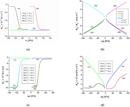
Figure 5.
Coefficients (i, j ∈ {1, 2, 3}, r = A, B) as functions of glucose osmotic pressure difference () and = 490.2 kPa: (a), and (b), (c), (d).
Figure 5b shows the dependencies = f(, = 490.2 kPa) and = f(, = 490.2 kPa). Curves 1A and 1B were obtained for the uniformity of the solutions and are symmetrical with respect to the axis passing through the point = 0. Curves 3A and 3B are characterized by symmetry with respect to the axis passing through the point = 0, which illustrate the dependences = f(, = 490.2 kPa) for the conditions of homogeneity of solutions and concentration polarization. Curves 2A and 2B show a slight asymmetry, which illustrate the dependence = f(, = 490.2 kPa) for the conditions of concentration polarization. The values of the coefficients are negative for both the uniformity of solutions and concentration polarization conditions. Moreover, the values of the coefficients for the concentration polarization conditions are slightly higher than for the concentration polarization conditions.
Figure 5c shows the dependencies = f(, = 490.2 kPa) and = f(, = 490.2 kPa). For the homogeneity conditions, the value of the coefficients and is independent of the concentration and configuration and is = = −0.68 × 10¹² N s mol−1. This case is illustrated in Figure 5c by curves 1A and 1B. For the conditions of concentration polarization, the values of the coefficients and are nonlinearly dependent on both and and the configuration of the membrane system, as illustrated by curves 2A and 2B as well as 3A and 3B. These graphs show that as the value of increases, the values of and are initially constant and amount to = −24.96 ×10⁹ N s mol−1 and = −24.36 ×10⁹ N s mol−1, and then for ≥ −110.29 kPa and ≥ 49.02 kPa increases to the value of = −1.54 ×10⁹ N s mol−1 and = −1.51 ×10⁹ N s mol−1. It should be noted that the coefficients and are negative. Disregarding the minus sign for (i.e., for ), the curves 2A and 2B as well as 3A and 3B intersect at the point with coordinates = 76.87 kPa and = = 3.21 ×10⁹ N s mol−1. This means that for this point, the value of and is the same for configurations A and B of the membrane system.
Figure 5d shows the dependence = f(, = 490.2 kPa). Curves 1A and 1B illustrate this relationship for the uniformity conditions of the solutions and configurations A and B of the membrane system. Curves 1A and 1B are symmetrical and curves 2A and 2B asymmetrical with respect to the axis passing through the point = 0. Disregarding the minus sign at (i.e., for ), the curves 2A and 2B intersect at the point with coordinates = 78.18 kPa and = 1.63 ×10⁹ mol2 N s m−3. This means that for this point, the value of is the same for configurations A and B of the membrane system.
Figure 6a shows the dependencies = f(, = 490.2 kPa) and = f(, = 490.2 kPa). The figure shows that for the homogeneity conditions of the solutions, the value of the coefficients is independent of the concentration and configuration of the membrane system and is = 2.04 ×10⁻³. This case is illustrated in Figure 6a by curves 1A and 1B. Curve 2A shows that for the concentration polarization conditions, the value of is constant and independent of . In contrast, the curve 2B shows that for the conditions of concentration polarization, the value of is constant and depends on . Figure 6a also shows that for the conditions of homogeneity of solutions, the value of the coefficients depends on but is independent on and the configuration. Curves 3A and 3B are symmetrical with respect to the axis passing through the point = 0.

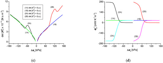
Figure 6.
Coefficients and (i, j ∈ {1, 2, 3}, r = A, B) as functions of glucose osmotic pressure difference () and = 490.2 kPa: and (a), (b), (c), and total production of entropy (r = A, B) (d).
Figure 6b shows the dependencies = f(, = 490.2 kPa). For the homogeneity conditions of the solutions the value of the coefficient is independent of the concentration and configuration of the membrane system, is constant and amounts to = 1.85 ×10⁷ m3 N s mol−2 (Figure 6, curves 1A and 1B). For the conditions of concentration polarization, the value of the coefficient is nonlinearly dependent on both and as well as the configuration, as illustrated by curves 2A and 2B. Curve 2A shows that as the value of increases, the value of is initially constant and amounts to = 66.23 ×10⁷ m3 N s mol−2, and then for > −110.29 kPa it decreases to values = 4.12 × 10⁷ m3 N s mol−2 (for ≥ −49.02 kPa). Similarly, the curve 2B shows that with the increase in the value of the value of is initially constant and amounts to = 66.23 ×10⁷ m3 N s mol−2, and then for > 49.02 kPa it decreases up to the value = 4.03 × 10⁷ m3 N s mol−2 (for ≥ 110.29 kPa). It should be noted that the coefficients are positive. Disregarding the minus sign for (i.e., for ), the curves 2A and 2B intersect at the coordinates = 78.75 kPa and = 8.72 ×10⁷ m3 N s mol−2. This means that for this point, the value of is the same for configurations A and B of the membrane system.
Figure 6c shows the dependence = f(, = 490.2 kPa). Curves 1A and 1B illustrate this dependence for the uniformity conditions of the solutions and configurations A and B. For concentration polarization, the value of the coefficient is nonlinearly dependent on both and as well as the configuration, as illustrated by curves 2A and 2B. Curves 1A and 1B are symmetrical, and curves 2A and 2B asymmetrical with respect to the axis passing through the point = 0. Curves 1A and 2A overlap in the range ≥ 28.12 kPa and ≤ −78.75 kPa. In contrast, the graphs 1B and 2B are the same for ≥ 80.62 kPa.
3.4. Calculations of the Global S-Entropy Source
Figure 6d shows the dependencies = f(, = 490.2 kPa) calculated based on Equation (A11). Curves 1A and 1B illustrate this dependence = f(, = 490.2 kPa) for the uniformity conditions of the solutions and configurations A and B. Curves 1A and 1B indicate that is independent of the concentration and configuration, and the value is approximately 30.5 mW K−1 m−2. For the concentration polarization conditions, the value of is nonlinear and depends both on and as well as on the configuration, as illustrated by curves 2A and 2B. Curve 2A shows that the value of is constant and amounts to approximately = 274.5 mW K−1 m−2 and then, for > −122.55 kPa, it decreases stepwise to the value of approximately = 2.21 mW K−1 m−2 for = −73.53 kPa. For > −73.53 kPa, curve 2A slightly decreases to the value of = 0.06 mW K−1 m−2. Curve 2B shows that the value of slightly decreases from the value of = 275.7 mW K−1 m−2 to the value of about = 208.67 mW K−1 m−2 and then, for > 61.27 kPa, it decreases stepwise to the value of about = 2.57 mW K−1 m−2 for = 85.78 kPa. For > −85.78 kPa, curve 2B slightly decreases to the value of = 0.01 mW K−1 m−2. Curves 3A and 3B illustrate the differences and as a result of the difference in the value of illustrated by curves 1A and 2A and the value of illustrated by curves 1B and 2B. Curves 3A and 3B, shown in Figure 6d, show that and are positive for 0 > ≥ −86.25 kPa and > 73.12 kPa, and negative for ≤ −86.25 kPa and < 73.12 kPa.
3.5. Osmotic Pressure Dependencies of
Figure 7 show the dependencies = f(, = 490.2 kPa) (i, j ∈ {1, 2, 3}, r = A, B) calculated based on Equation (A14) and data presented in Figure 4, Figure 5a–d and Figure 6a–c. Figure 7a shows that the value of the coefficients and increases approximately linearly with the increase of . The largest increase occurs for the coefficients and for the concentration polarization conditions (curves 2A and 3A). In turn, the value of the coefficients and for the conditions of homogeneity of solutions increases nonlinearly with the increase of . For the conditions of concentration polarization, the values of the coefficients and initially increase nonlinearly and reach the maximum values of = 0.05 for = 45.94 kPa (curve 2B) and = 0.052 for = 59.06 kPa (curve 3B) and then decrease and increase again. Curves 1A and 1B obtained for the uniformity of solutions are symmetrical with respect to the vertical axis passing through the point = 0 and = = = = = . In contrast, the curves 2A and 2B as well as 3A and 3B obtained for the conditions of concentration polarization of the solutions are asymmetric with respect to the vertical axis passing through the point = 0, and > > = , > > = and > > > > = .
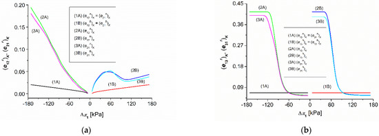
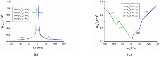
Figure 7.
The (c) (i, j ∈ {1, 2, 3}, r = A, B) coefficients as functions of glucose osmotic pressure difference () with = 490.2 kPa: and (a), and (b), (c), (d).
Curves 1A and 1B shown in Figure 7b show that for the uniformity of solutions, the values of the coefficients , , , are independent of for = ±490.2 kPa. Moreover, for the homogeneity condition, = = = . In contrast, for the conditions of concentration polarization, the values of the coefficients , , , are initially constant and amount to = 0.41, = 0.39, = 0.41 and = 0.39. Then, for > −121.87 kPa, the values of and initially decrease to the value = = 0.11 for = −77.81 kPa and then asymptotically to the value of = = 0.056. Similarly, for > 43.12 kPa, the values of and initially decrease to the value of = = 0.11 for = 77.81 kPa and then asymptotically to the value of = = 0.055. The curves 2A and 2B intersect at the point with coordinates = 77.81 kPa and = = = . This means that for this point, the values of = = = are the same for A and B configurations in concentration polarization conditions.
Figure 7c, d shows the dependencies = f(, = 490.2 kPa) and = f(, = 490.2 kPa) (r = A, B), respectively. Curves 1A and 1B in Figure 7c illustrate this dependence for the homogeneity conditions of the solutions and configurations A and B. For the conditions of concentration polarization, the value of the coefficient is nonlinearly dependent on both and and the configuration of the membrane system, as illustrated by curves 2A and 2B. Curves 1A and 1B are symmetrical, and curves 2A and 2B are asymmetric with respect to the vertical axis passing through the point = 0. Figure 7d shows that the dependence = f(, = 490.2 kPa) is the same for both the homogeneity of solutions and polarization conditions.
3.6. Calculations of F-Energy in the Membrane System
Figure 8 shows the dependencies = f(, = 490.2 kPa) calculated based on Equation (A15). Curves 1A and 1B presented in Figure 8a illustrate the dependence = f(, = 490.2 kPa) for the conditions of homogeneity of solutions and configuration A and B. As shown, is linearly dependent on the concentration of the solutions and the configuration of the membrane system. Additionally, = . For the concentration polarization conditions, the value is nonlinear and depends both on and and on the configuration as illustrated by curves 2A and 2B. Curve 2A shows that the value decreases nonlinearly from the value = 19.5 Wm−2 to the constant value = 0.1 mWm−2, for > −49.02 kPa. Curve 2B shows that the value initially increases nonlinearly, and when obtaining the maximum value = 3.63 Wm−2 (for = 36.8 kPa), decreases nonlinearly to the value = 0.21 Wm−2 (for = 73.8 kPa). For > 73.8 kPa, increases linearly. Similar changes in the dependence occur for and , as illustrated by the curves 3A and 3B. In the areas where and reach the highest values, the condition > is fulfilled.
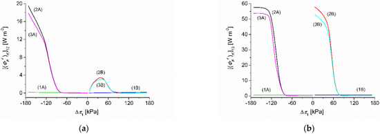

Figure 8.
Total production of free energy , (i, j ∈ {1, 2, 3}, r = A, B) as functions of osmotic pressure difference of glucose () with a constant osmotic pressure of ethanol ( = 490.3 kPa) and = 0: = (a), = (b), (c), (d).
Figure 8b shows the dependencies = f(, = 490.2 kPa) calculated based on Equation (A13). Curves 1A and 1B illustrate this dependence for the uniformity conditions of the solutions and configurations A and B. These graphs indicate that is independent of the concentration and configuration, and the value is approximately 0.6 Wm−2. In addition, = . For the conditions of the concentration polarization, the characteristic = f(, = 490.2 kPa) is nonlinear and dependent on both and as well as the configuration, as illustrated by curves 2A and 2B. Curve 2A shows that initially the value of decreases linearly from approximately = 57.53 Wm−2 to = 37.18 Wm−2 and then, for > −110.29 kPa, it decreases stepwise to a constant value of approximately = 1.1 mWm−2 for = −24.51 kPa. Curve 2B shows that the value decreases from the value = 57.78 Wm−2 to approximately = 0.2 mWm−2, for = 122.52 kPa. In turn, for > 122.52 kPa, is constant. Similar changes occur for and , as illustrated by the curves 3A and 3B shown in Figure 8b. This figure shows that > .
Curves 1A and 1B shown in Figure 8c illustrate the dependence = f(, = 490.2 kPa) for the conditions of homogeneity of solutions and configuration A and B. These curves indicate that are nonlinearly dependent on the concentration of the solutions and not dependent on the configuration of the membrane system. Curve 2A shows that the value initially increases linearly, and, after reaching the maximum value = 6.37 mW m−2 (for = 6.13 kPa), decreases nonlinearly to the value = 1.04 mW m−2 (for = 36.76 kPa), and then increases to the second maximum = 1.61 mW m−2 (for = 49.02 kPa). For > 49.02 kPa, is constant and amounts to 0.6 mW m−2.
Curves 1A and 1B shown in Figure 8d illustrate the relationship = f(, = 490.2 kPa) for the conditions of homogeneity of solutions and configuration A and B. These curves indicate that are nonlinearly dependent on the concentration of the solutions and not dependent on the configuration of the membrane system. For the conditions of concentration polarization, the values of are nonlinear and depend on both and and the configuration, as illustrated by curves 2A and 2B. Curve 2A shows that the value decreases nonlinearly from the value = 58.54 μWm−2 to the value w approximation of the constant = 0.07 μWm−2, for > −49.02 kPa. Curve 2B shows that the value initially increases nonlinearly, and after reaching the maximum value = 16.84 μWm−2 (for = 36.8 kPa), decreases nonlinearly to the value = 0.2 μWm−2 (for = 98.1 kPa). For > 98.1 kPa, is constant. Figure 8d shows that in the areas where and reach the highest values, the condition > is fulfilled. Figure 8 shows that is of the same order of magnitude as , whereas is three orders of magnitude smaller than and one order of magnitude larger than .
Nonlinear changes in the values of , and (k = 1, 2 and r = A, B) in different ranges , depending on the configuration of the membrane system, are the source of the nonlinearity of the coefficients , and (i, j ∈ {1, 2, 3} and r = A, B). These coefficients are illustrated by curves 2A and 2B in Figure 5a–d, Figure 6a–c and Figure 7a–d. These nonlinearities are a consequence of the diffusive creation of CBLs or their destruction by free convection. In the convection-free state, is minimized, and in the convective state, CBLs, due to their partial destruction by natural convection, partially rebuild . The appearance of convective flows depends on the return of the density gradient of the solutions located in the membranous areas in relation to . If a density of a solution above the membrane is lower than a density of a solution below the membrane, it is a non-convective state. Otherwise, it is a convective state.
Nonlinear dependences, presented in the paper, are a consequence of pseudophase transitions from non-convective to convective states or vice versa. The non-convective state that occurs in the conditions of concentration polarization, masks the Earth’s gravity. Therefore, the non-convective state corresponds to the microgravity conditions that occur during orbital travel in outer space. In turn, the convective state occurs in planetary (e.g., terrestrial) conditions. Therefore, it is a gravitational effect [44]. The gravitational field requires living organisms to adapt in the form of antigravity systems such as the heart, skin and skeleton [45].
In the study of energy transformations in systems in which the membrane structure contains micro- or nanochannels, many effects are observed, such as spherical interactions near proteins or electrodes in electrochemical cells [46], ion-substrate coupling or the formation of an occludic state with high affinity with ionic compounds and the substrate [47]. It has also been observed that viscoelectric modifications of the electrolyte can change the electroosmotic mobility and electrical conductivity of the nanochannel [48]. Moreover, it was found that the hysteresis and electroosmotic flows influence ion transport in micro-flow devices [49,50].
The method of F-energy determination that we proposed in this paper for cellulose membranes can also be used to characterize other membrane systems, in which a solution is transported through the membrane in osmotic-diffusive transport. To calculate F-energy for other membrane systems, it is needed to determine the transport properties of a studied membrane and fluxes of solutions that are being transported. Determined F-energy in concentration polarization conditions may be applied to optimize parameters of membrane dressings used in biomedicine to improve healing processes, such as bacterial cellulose or Textus Bioactiv, that support the treatment of difficult-to-heal wounds (burns, venous leg ulcers) and constitute a barrier between the wound surface and its surroundings [51,52,53]. Additional applications include the optimization of drug penetration from microemulsions applied on the surface of a flat polymer membrane used in ophthalmology and laryngology [54] and used as drug carriers in the prophylaxis of fungal infections in chronic wounds [6]. Other membrane systems used as drug carriers are polymer hydrogels and nanoparticles that include liposomes, nanomicelles or dendrimers [5] that enable controlled drug delivery. Additionally, a system consisting of packed gel beads immersed in water was used as a model for the release of antibiotics [55].
The results presented here, could also be used for novel membrane systems that produce energy. Determining the F-energy would designate whether a certain membrane system is able to produce F-energy that can be used for energy-consuming processes such as active membrane transport. Different versions of the phenomena of osmosis and diffusion have been used in osmotic pumps as osmotic drug delivery systems [56] and in an osmotic pump and osmotic engine [57,58].
In our membrane model, we use Equation (A9) to determine energy conversion from U-energy to F-energy and S-energy for isothermal–isochoric processes. For isothermal–isobaric processes, Equation (A9) can be written as
where is the flux of enthalpy, is the flux of free enthalpy and is the flux of dissipated energy (S-energy). For liquid and solid = and = , Equation (5) and the procedure proposed in this paper can be used to evaluate the energy conversion accompanying biochemical reactions. In this case, the direction and extent of occurrence of these reactions depends on the combination of components present in Equation (5). The component plays the main role. The transport and energy considerations presented in this paper can be extended by considering other thermodynamic forces and fluxes [29,59,60].
The internal energy (U-energy), which was subject to conversion in our model, is limited to chemical energy. The unsurpassed converter of chemical energy (U-energy) directly into useful energy (F-energy) is a biological cell functioning like a chemodynamic machine. The conversion of F-energy contained in the chemical bonds of macromolecules into high-energy compounds such as adenosine triphosphate (ATP) is crucial to useful work including mechanical, osmotic, electrical or biosynthesis work [61]. The production of S-energy is dependent on the rate of biochemical processes: the slower the process, the greater the efficiency of the cell. The role of slowing down the rate of transport processes is fulfilled by concentration polarization.
Chang and co-authors demonstrate the feasibility of using membrane processes to enhance bioenergy production [62]. The literature review, which is a small compendium of knowledge and experience in the field of bioenergy production, provides an incentive to develop a research direction thematically related to one of the most important scientific challenges in the world.
4. Conclusions
The form of the Kedem–Katchalsky–Peusner model equations, containing the Peusner coefficients , enables the analysis of energy conversion in membrane systems to study the transport properties of membranes. The coefficients are dependent on the concentration of the solutions separated by the membrane and the configuration of the membrane system. The analysis of energy conversion in membrane systems consists of calculating the free energy (F-energy) based on the expression containing the production of S-entropy () and the energy conversion efficiency coefficient (). To calculate the entropy production (), it is necessary to calculate the coefficients and the flux and . The coefficients allow the calculation of the energy conversion coefficients . The energy conversion efficiency can be calculated from the coefficients . The largest amount of F-energy appears when, in the equation for , there is a coefficient or .
The systems described in this paper require energy to function. Energy conversion is the process of changing energy from one form to another. The process is the same in micro- and macrosystems. Each subsequent stage of conversion may reduce the efficiency of the system. Therefore, proper energy management is essential. Energy management is a combination of various measures ensuring that the required performance is achieved with minimum energy expenditure. Appropriate management allows optimization of the processes of energy production, its consumption, avoiding energy drops and reducing energy losses.
This paper presents a thermodynamic model taking into account concentration polarization and results of studies on transport and F-energy estimation in membrane systems. These results can provide a basis for investigating the transport properties of new polymeric membranes, modified with nanoparticles, providing an increase in hydraulic performance while maintaining high separation efficiency and controlling the phenomenon of pore blockage. In addition, the obtained results can be used to modernize existing technologies, which is one of the most important elements of designing technological concepts in the management of an enterprise, especially thermal and utility power plants and enterprises where boiler and district heating systems and water-cooling systems are operated. For these purposes, water preparation plants are used in which membrane separation plays an important role as a unit process. Therefore, the correct operation of these plants is an important part of process management in the power industry. It should be emphasized that water consumption in the processes of the production and supply of electricity, gas, steam and hot water in Poland is 5.55 × 10⁵ m3 annually, which is 88% of the water consumption in industry. The preparation of water for these purposes in highly efficient processes allows for multiple uses of water and savings in “fresh” water consumption, which, in consequence, brings economic and environmental benefits and is in accordance with the principles of the closed-cycle economy.
Author Contributions
Conceptualization, K.M.B.; methodology, K.M.B., A.Ś. and I.Ś.-P.; software, K.M.B.; formal analysis: K.M.B., A.Ś., I.Ś.-P. and W.M.B.; investigation, K.M.B., A.Ś., I.Ś.-P. and W.M.B.; resources, K.M.B., A.Ś., I.Ś.-P. and W.M.B.; data curation, K.M.B., A.Ś.; writing—original draft preparation, K.M.B., A.Ś., I.Ś.-P. and W.M.B., writing—review and editing, K.M.B., A.Ś., I.Ś.-P., W.M.B. and M.W.-M.; visualization, K.M.B. and A.Ś.; supervision, A.Ś.; funding acquisition, W.M.B. and M.W.-M. All authors have read and agreed to the published version of the manuscript.
Funding
The scientific research was funded by the statute subvention of Czestochowa University of Technology.
Data Availability Statement
The datasets for this study are available on request to the corresponding author.
Acknowledgments
We would like to thank those who have touched our science paths.
Conflicts of Interest
The authors declare no conflict of interest.
List of Symbols
| Jv | volume flux (m s−1); |
| Jl, Jm, Jh | solute fluxes (mol m−2s−1); |
| Il, Is, Im, Ih | ionic currents (A); |
| hydraulic conductivity coefficient (m−3 N−1 s−1); | |
| reflection coefficient; | |
| electroosmotic permeability coefficient (NA−1) | |
| ω | solute permeability coefficient (mol N−1 s−1); |
| γ | van’t Hoff coefficient; |
| R | gas constant (J mol−1 K−1); |
| T | absolute temperature (K); |
| electrical conductivity (Ω−1 m−2); | |
| transfer number; | |
| valence; | |
| ion number; | |
| average concentration of the solution (mol m−3); | |
| potential difference measured with two reversible electrodes (V); | |
| , | transfer number of anions (a) and cations (c) in the membrane; |
| t | time (s); |
| and | concentration boundary layers; |
| δl, δh | thickness of the concentration boundary layers (m); |
| δm | membrane thickness (m); |
| mechanical pressure difference (Pa); | |
| CBLs | concentration boundary layers; |
| g | acceleration due to the fact of gravity (m s−2); |
| , | diffusion coefficients (m2 s−1); |
| , | the kinematic viscosity coefficients (m2 s−1); |
| , | solution concentrations at the boundaries of M/ and M/ (mol m−3); |
| , | solution densities at the boundaries of M/ and M/ (kg m−3); |
| , | solution concentrations beyond and (mol m−3); |
| , | solution densities beyond and (kg m−3). |
| F | free energy (W m−2) |
| U | internal energy (W m−2) |
| global source of entropy (W K−1 m−2) | |
| energy conversion efficiency coefficient | |
| coefficient of concentration polarization |
Appendix A
The Kr form of Kedem–Katchalsky–Peusner equations for non-electrolyte solutions in concentration polarization conditions
Taking into account Equation (1), we can write Equations (2) and (3) in the following forms
where , , , .
Compared to Equations (2) and (3), the coefficients and appear in the first and second components of Equations (A1) and (A2) and ∆P appears in the third component instead .
It appears from Equations (1)–(3) that seven coefficients are needed to characterize the membrane transport processes of ternary non-electrolytic solutions. These coefficients are defined by the equations listed in Table A1.

Table A1.
Physical interpretation of membrane transport parameters.
Table A1.
Physical interpretation of membrane transport parameters.
| Coefficient | Definition | |
|---|---|---|
In turn, Equations (1)–(3) show that twelve concentration polarization coefficients are needed to characterize the stochastic polarization in a membrane system containing ternary non-electrolyte solutions. The definitions of these coefficients are summarized in Table A2.
Table A2.
Physical interpretation of concentration polarization coefficients.
Table A2.
Physical interpretation of concentration polarization coefficients.
| Coefficient | Definition | |
|---|---|---|
In the definitions summarized in Table A2, , , , , and refer to the homogeneity conditions of the solutions. To obtain the expressions for , we use the third component of Equations (2) and (3) or (4) and (5) for concentration polarization conditions and solution homogeneity conditions. For Equations (2) and (3), we obtain and . For Equations (4) and (5), we obtain and . In these equations, , , and .
Relatively simple algebraic transformations enable transformation of Equations (1)–(3) into the form
where: ,
,
,
,
,
,
,
,
.
Equations (A1)–(A3) can be written in a matrix form
where [] is a matrix of Peusner coefficients (i, j ∈ {1, 2, 3}) for ternary solutions of non-electrolytes and concentration polarization conditions. Equations (A1)–(A3) are one of the forms of the Kedem–Katchalsky equations obtained by means of the hybrid transformation of Peusner thermodynamic networks for the conditions of concentration polarization. The comparison of Equations (A1)–(A3) shows that for non-diagonal coefficients ≠ , ≠ and ≠ . In turn, we treat the determinant of the matrix [] as the coefficient
The index “r” in Equations (1)–(3) and (A1)–(A7) means that the fluxes , , , the coefficients and (i, j ∈ {1, 2, 3} and r = A, B) depend on the configuration of the membrane system. In Equations (1)–(3) and (A1)–(A5) for the homogeneity conditions, the superscript “r” is omitted and the following condition are assumed = = = = = = = = = 1.
Mathematical model of energy conversion in the membrane system.
In thermodynamic systems, including membrane systems, internal energy (U) consist of free energy (F) and dispersed energy (TS, T—absolute temperature, S—thermodynamic entropy) [7,25]. The rates of change of these variables are related by the equation
where is the rate at which entropy is created in the membrane system by irreversible processes and is the rate of entropy flow to the environment. Assuming that = 0, we have = . Dividing both sides of this equation by A, we obtain the equation for the conditions of concentration polarization [25]
where —internal energy flux (–energy), – free energy flux (-energy), is the dissipated energy flux (function of energy dissipation per unit area) (-energy) and = .
If the solutions contain a solvent and two dissolved substances, then the global source of entropy for the concentration polarization conditions denoted by is described by the equation [40]
where is the global source of entropy for concentration polarization conditions, is the S-entropy produced by , is the S-entropy produced by , and are the volume and solute fluxes, respectively, for the concentration polarization conditions of the solutions, r = A or B means the configuration of the membrane system, k = 1, 2).
Considering Equations (A3)–(A5) in Equation (A8), we obtain
where: , , , , , ,
Equation (A11) shows the version of the global entropy source for the concentration polarization conditions (). The product is the flux of dissipated energy, i.e., the time change of energy per unit area of the membrane expressed in J/m2 s or W/m2. We can calculate the free energy flux for the concentration polarization conditions using the expression below [25]
By transforming the above expression, we obtain
where: is the energy conversion efficiency by means of the Kedem–Caplan–Peusner coefficient [17,41], which can be presented in the following form
The values of the coefficients are limited by the relation 0 ≤ ≤ +1. Taking into account the Equation (A14) in (A10) we obtain
From the above procedure based on Equations (A13)—(A15), we can calculate the amount of available free energy that can be converted into useful work or other types of energy. It should be noted that to obtain Equations (A9)–(A15) for the homogeneity conditions of solutions, it is enough to leave the superscript “r” in these equations.
References
- Demirel, Y. Nonequilibrium Thermodynamics:Transport and Rate Processes in Physical, Chemical and Biological Systems; Elsevier: Amsterdam, The Netherlands, 2014. [Google Scholar]
- Uragami, T. Science and Technology of Separation Membranes; John Wiley & Sons: Chichester, UK, 2017. [Google Scholar]
- Baker, R. Membrane Technology and Application; John Wiley & Sons: New York, NY, USA, 2012. [Google Scholar]
- Gerbaud, V.; Shcherbakova, N.; Da Cunha, S. A nonequilibrium thermodynamics perspective on nature-inspired chemical engineering processes. Chem. Eng. Res. Des. 2020, 154, 316–330. [Google Scholar] [CrossRef]
- Raghuvanshi, S.; La Prairie, B.; Rajagopal, S.; Yadav, V.G. Polymeric nanomaterials for ocular drug delivery. In Advances in Polymeric Nanomaterials for Biomedical Applications; Bajpai, A.K., Saini, R.K., Eds.; Elsevier: Amsterdam, The Netherlands, 2021; pp. 309–325. [Google Scholar] [CrossRef]
- Rewak-Soroczynska, J.; Sobierajska, P.; Targonska, S.; Piecuch, A.; Grosman, L.; Rachuna, J.; Wasik, S.; Arabski, M.; Ogorek, R.; Wiglusz, R.J. New approach to antifungal activity of fluconazole incorporated into the porous 6-Anhydro-α-L-Galacto-β-D—Galactan structures modified with nanohydroxyapatite for chronic-wound treatments—In vitro evaluation. Int. J. Mol. Sci. 2021, 22, 3112. [Google Scholar] [CrossRef]
- Katchalsky, A.; Curran, P.F. Nonequilibrium Thermodynamics in Biophysics; Harvard University Press: Cambridge, UK, 1965. [Google Scholar]
- Cheng, X.; Pinsky, P.M. The balance of fluid and osmotic pressures across active biological membrane with application to the corneal endothelium. PLoS ONE 2015, 10, e0145422. [Google Scholar] [CrossRef] [PubMed]
- Wijmans, J.G.; Baker, W. The solution-diffusion model: A review. J. Membr. Sci. 1995, 107, 1–21. [Google Scholar] [CrossRef]
- Al-Obaidi, M.A.; Kara-Zaitri, C.; Mujtaba, I.M. Scope and limitation of the irreversible thermodynamics and the solution diffusion models for the separation of binary and multi-component systems in reverse osmosis process. Comput. Chem. Eng. 2017, 100, 48–79. [Google Scholar] [CrossRef]
- Spiegler, K.S. Transport processes in ionic membranes. Trans. Faraday Soc. 1958, 54, 1408–1428. [Google Scholar] [CrossRef]
- Kedem, O.; Katchalsky, A. A physical interpretation of the phenomenological coefficients of membrane permeability. J. Gen. Physiol. 1961, 45, 143–179. [Google Scholar] [CrossRef]
- Ślęzak, A. A frictional interpretation of the phenomenological coefficients of membrane permeability for multicomponent non-ionic solutions. J. Biol. Phys. 1997, 23, 239–250. [Google Scholar] [CrossRef]
- Friedman, H.; Meyer, R.A. Transport across homoporous and heteroporous membranes in nonideal, nondilute solutions. I. Inequality of reflection coefficients for volume flow and solute flow. Biophys. J. 1981, 34, 535–544. [Google Scholar] [CrossRef]
- Mason, E.A.; Lonsdale, H.K. Statistical-mechanical theory of membrane transport. J. Memb. Sci. 1990, 51, 1–81. [Google Scholar] [CrossRef]
- Oster, G.; Perelson, A.; Katchalsky, A. Network thermodynamics. Nature 1971, 234, 239–399. [Google Scholar] [CrossRef]
- Peusner, L. Studies in Network Thermodynamics; Elsevier: Amsterdam, The Netherlands, 1986. [Google Scholar]
- Batko, K.M.; Ślęzak-Prochazka, I.; Grzegorczyn, S.; Ślęzak, A. Membrane transport in concentration polarization conditions: Network thermodynamics model equations. J. Porous Media 2014, 17, 573–586. [Google Scholar] [CrossRef]
- Ślęzak-Prochazka, I.; Batko, K.M.; Wąsik, S.; Ślęzak, A. H* Peusner’s form of the Kedem-Katchalsky equations fornon-homogeneous non-electrolyte binary solutions. Transp. Porous Media 2016, 111, 457–477. [Google Scholar] [CrossRef]
- Ślęzak, A.; Grzegorczyn, S.; Batko, K.M. Resistance coefficients of polymer membrane with concentration polarization. Transp. Porous Media 2012, 95, 151–170. [Google Scholar] [CrossRef]
- Batko, K.M.; Ślęzak-Prochazka, I.; Ślęzak, A. Network hybrid form of the Kedem-Katchalsky equations for non-homogenous binary non-electrolyte solutions: Evaluation of Pij* Peusner’s tensor coefficients. Transp. Porous Media 2015, 106, 1–20. [Google Scholar] [CrossRef]
- Batko, K.; Ślęzak, A. Membrane transport of nonelectrolyte solutions in concentration polarization conditions: Hr form of the Kedem–Katchalsky–Peusner equations. Int. J. Chem. Eng. 2019, 2019, 5629259. [Google Scholar] [CrossRef]
- Ślęzak, A.; Grzegorczyn, S.; Batko, K.M.; Bajdur, W.M.; Makuła-Włodarczyk, M. Applicability of the Lr form of the Kedem–Katchalsky–Peusner equations for membrane transport in water purification technology. Desalin. Water Treat. 2020, 202, 48–60. [Google Scholar] [CrossRef]
- Batko, K.; Ślęzak, A.; Grzegorczyn, S.; Bajdur, W.M. The Rr form of the Kedem–Katchalsky–Peusner model equations for description of the membrane transport in concentration polarization conditions. Entropy 2020, 22, 857. [Google Scholar] [CrossRef]
- Batko, K.; Ślęzak, A.; Pilis, W. Evaluation of transport properties of biomembranes by means of Peusner network thermodynamics. Acta Bioeng. Biomech. 2021, 23, 63–72. [Google Scholar] [CrossRef]
- Kargol, M.; Kargol, A. Mechanistic formalism for membrane transport generated by osmotic and mechanical pressure. Gen. Physiol. Biophys. 2003, 22, 51–68. [Google Scholar]
- Peusner, L. The Principles of Network Thermodynamics: Theory and Biophysical Applications. Ph.D. Thesis, Harvard University, Cambridge, MA, USA, 1970. [Google Scholar]
- Peusner, L. Hierarchies of irreversible energy conversion systems: A network thermodynamics approach. I. Linear steady state without storage. J. Theor. Biol. 1983, 10, 27–39. [Google Scholar] [CrossRef]
- Peusner, L. Hierarchies of irreversible energy conversion systems. II. Network derivation of linear transport equations. J. Theor. Biol. 1985, 115, 319–335. [Google Scholar] [CrossRef]
- Peusner, L. Network representation yelding the evolution of Brownian motion with multiple particle interactions. Phys. Rev. A 1985, 32, 1237–1238. [Google Scholar] [CrossRef]
- Peusner, L.; Mikulecky, D.C.; Caplan, S.R. A network thermodynamic approach to Hill and King-Altman reaction-diffusion kinetics. J. Chem. Phys. 1985, 83, 5559–5566. [Google Scholar] [CrossRef]
- Ślęzak, A.; Dworecki, K.; Ślęzak, I.H.; Wąsik, S. Permeability coefficient model equations of the complex: Membrane-concentration boundary layers for ternary nonelectrolyte solutions. J. Membr. Sci. 2005, 267, 50–57. [Google Scholar] [CrossRef]
- Ślęzak, A.; Grzegorczyn, S.; Jasik-Ślęzak, J.; Michalska-Małecka, K. Natural convection as an asymmetrical factor of the transport through porous membrane. Transp. Porous Media 2010, 84, 685–698. [Google Scholar] [CrossRef]
- Dworecki, K.; Ślęzak, A.; Ornal-Wąsik, B.; Wąsik, S. Effect of hydrodynamic instabilities on solute transport in a membrane system. J. Membr. Sci. 2005, 265, 94–100. [Google Scholar] [CrossRef]
- Jasik-Ślęzak, J.; Olszówka, K.M.; Ślęzak, A. Estimation of thickness of concentration boundary layers by osmotic volume flux determination. Gen. Physiol. Biophys. 2011, 30, 186–195. [Google Scholar] [CrossRef]
- Ślęzak, A. Irreversible thermodynamic model equations of the transport across a horizontally mounted membrane. Biophys. Chem. 1989, 34, 91–102. [Google Scholar] [CrossRef]
- Ślęzak, A.; Dworecki, K.; Jasik-Ślęzak, J.; Wąsik, J. Method to determine the practical concentration Rayleigh number in isothermal passive membrane transport processes. Desalination 2004, 168, 397–412. [Google Scholar] [CrossRef]
- Ślęzak, A.; Dworecki, K.; Anderson, J.A. Gravitational effects on transmembrane flux: The Rayleigh-Taylor convective instability J. Membr. Sci. 1985, 23, 71–81. [Google Scholar] [CrossRef]
- Ewing, G.W. Instrumental Methods of Chemical Analysis; McGraw-Hill Book Company: New York, NY, USA, 1985. [Google Scholar]
- Batko, K.M.; Ślęzak, A. Evaluation of the global S-entropy production in membrane transport of aqueous solutions of hydrochloric acid and ammonia. Entropy 2020, 22, 1021. [Google Scholar] [CrossRef] [PubMed]
- Kedem, O.; Caplan, S.R. Degree of coupling and its relation to efficiency of energy conversion. Trans. Faraday Soc. 1965, 61, 1897–1911. [Google Scholar] [CrossRef]
- Grzegorczyn, S.; Ślęzak, A.; Przywara-Chowaniec, B. Concentration polarization phenomenon in the case of mechanical pressure difference on thr membrane. J. Biol. Phys. 2017, 43, 225–238. [Google Scholar] [CrossRef] [PubMed]
- Lebon, G.; Jou, D.; Casas-Vasquez, J. Understanding Non-Equilibrium Thermodynamics Foundations, Applications, Frontiers; Springer: Berlin, Germany, 2008. [Google Scholar]
- Batko, K.M.; Ślęzak, A.; Bajdur, W.M. The role of gravity in the evolution of the concentration field in the elekctrochemical membrane cell. Entropy 2020, 22, 680. [Google Scholar] [CrossRef] [PubMed]
- Adampolous, K.; Koutsouris, D.; Zaravinous, A.; Lambrou, G.I. Gravitational influence on human living systems and the evolution of spaces on earth. Molecules 2021, 26, 2784. [Google Scholar] [CrossRef] [PubMed]
- Horng, T.-L.; Lin, T.-C.; Liu, C.; Eisenberg, B. PNP Equations with steric effects: A model of ion flow through channels. J. Phys. Chem. B 2012, 116, 11422–11441. [Google Scholar] [CrossRef]
- Caplan, D.A.; Subbotina, J.O.; Noskov, S.Y. Molecular mechanism of ion-ion and ion-substrate coupling in the Na+-dependent leucine transporter LeuT. Biophys. J. 2008, 95, 4613–4621. [Google Scholar] [CrossRef]
- Hsu, W.-L.; Harvie, D.J.E.; Davidson, M.R.; Dunstan, D.E.; Hwang, J.; Daiguji, H. Viscoelectric fffects in nanochannel electrokinetics. J. Phys. Chem. C 2017, 121, 20517–20523. [Google Scholar] [CrossRef]
- Lim, A.E.; Lim, C.Y.; Lam, Y.C. Electroosmotic flow hysteresis for dissimilar anionic solutions. Anal. Chem. 2016, 88, 8064–8073. [Google Scholar] [CrossRef]
- Lim, A.E.; Lam, Y.C. Numerical investigation of nanostructure orientation on electroosmotic flow. Micromachines 2020, 11, 971. [Google Scholar] [CrossRef] [PubMed]
- Ullah, H.; Santos, H.A.; Khan, T. Applications of bacterial cellulose in food, cosmetics and drug delivery. Cellulose 2016, 23, 2291–2314. [Google Scholar] [CrossRef]
- Kucharzewski, M.; Wilemska-Kucharzewska, K.; Kózka, M.; Spałkowska, M. Leg venous ulcer healing process after application of membranous dressing with silver ions. Phlebologie 2013, 42, 340–346. [Google Scholar] [CrossRef]
- Ślęzak, A.; Kucharzewski, M.; Franek, A.; Twardokęs, W. Evaluation of the efficiency of venous leg ulcer treatment with a membrane dressing. Med. Eng. Phys. 2004, 26, 2653–2660. [Google Scholar] [CrossRef]
- Richter, T.; Keipert, S. In vitro permeation studies comparing bovine nasal mucosa, porcine cornea and artificial membrane: Androstenedione in microemulsions and their components. Eur. J. Pharm. Biopharm. 2004, 58, 137–143. [Google Scholar] [CrossRef]
- Kosztolowicz, T.; Dutkiewicz, A.; Lewandowska, K.D.; Wasik, S.; Arabski, M. Subdiffusion equation with Caputo fractional derivative with respect to another function in modelling diffusion in a complex system consisting of matrix and channels. Phys. Rev. E 2021, 104, 014118. [Google Scholar] [CrossRef]
- Lim, M.Y.; Roach, J.O. Metabolism and Nutrition; Elsevier: Edinburg, TX, USA, 2007. [Google Scholar]
- Patel, J.; Shalin Parikh, S.; Patel, S. Comprehensive review on osmotic drug delivery system. World J. Pharm. Res. 2021, 10, 523–550. [Google Scholar] [CrossRef]
- Delmotte, M.; Chanu, J. Non-equilibrium thermodynamics and membrane potential measurement in biology. In Topics Bioelectrochemistry and Bioenergetics; Millazzo, G., Ed.; John Wiley & Sons: Chichester, UK, 1979; pp. 307–359. [Google Scholar]
- Hoshiko, T.; Lindley, B.D. Phenomenological description of active transport of salt and water. J. Gen. Physiol. 1967, 50, 729–758. [Google Scholar] [CrossRef]
- Bui, T.Q.; Magnussen, O.-P.; Cao, V.D.; Wang, W.; Kjøniksen, A.-L.; Aaker, O. Osmotic engine converting energy from salinity difference to a hydraulic accumulator by utilizing olyelectrolyte hydrogels. Energy 2021, 232, 121055. [Google Scholar] [CrossRef]
- Sharma, M.; Chakraborty, A.; Purkait, M.K. Clean energy from salinity gradients using pressure retarded osmosis and reverse electrodialysis: A review. Sustain. Energy Technol. Assess. 2022, 49, 101687. [Google Scholar] [CrossRef]
- Chang, H.; Zou, Y.; Hu, R.; Feng, H.; Wu, H.; Zhong, N.; Hu, J. Membrane applications for microbial energy conversion: A review. Environ. Chem. Lett. 2020, 18, 1581–1592. [Google Scholar] [CrossRef]


Publisher’s Note: MDPI stays neutral with regard to jurisdictional claims in published maps and institutional affiliations. |
© 2022 by the authors. Licensee MDPI, Basel, Switzerland. This article is an open access article distributed under the terms and conditions of the Creative Commons Attribution (CC BY) license (https://creativecommons.org/licenses/by/4.0/).