Predicting the Compressibility Factor of Natural Gas by Using Statistical Modeling and Neural Network

Abstract

Simulating the phase behavior of a reservoir fluid requires the determination of many parameters, such as gas–oil ratio and formation volume factor. The determination of such parameters requires knowledge of the critical properties and compressibility factor (Z factor). There are many techniques to determine the compressibility factor, such as experimental pressure, volume, and temperature (PVT) tests, empirical correlations, and artificial intelligence approaches. In this work, two different models based on statistical regression and multi-layer-feedforward neural network (MLFN) were developed to predict the Z factor of natural gas by utilizing the experimental data of 1079 samples with a wide range of pseudo-reduced pressure (0.12–25.8) and pseudo reduced temperature (1.3–2.4). The statistical regression model was proposed and trained in R using the “rjags” package and Markov chain Monte Carlo simulation, while the multi-layer-feedforward neural network model was postulated and trained using the “neural net” package. The neural network consists of one input layer with two anodes, three hidden layers, and one output layer. The input parameters are the ratio of pseudo-reduced pressure and the pseudo-reduced temperature of the natural hydrocarbon gas, while the output is the Z factor. The proposed statistical and MLFN models showed a positive correlation between the actual and predicted values of the Z factor, with a correlation coefficient of 0.967 and 0.979, respectively. The results from the present study show that the MLFN can lead to accurate and reliable prediction of the natural gas compressibility factor.

1. Introduction

The relationship between pressure, volume, and temperature can be summarized by the equation of state (EOS). EOS has been widely used in the petroleum industry, especially when dealing with natural gas. Natural gas reservoirs play a vital role in responding to the massive global energy market. Knowledge of the physical properties of gas or oil related to pressure, volume, and temperature (PVT) is of great importance to petroleum engineers and academics. The physical properties of natural gas, which are used in the estimation of hydrocarbon reserves in reservoirs, the study of gas flow in the reservoir and wellbore and its thermodynamic behavior are essential in planning, gas metering, the design of pipelines, and surface facilities [1]. Most of these properties can be determined in a PVT laboratory. One of the most important properties is the compressibility factor of a gas, because most of the other hydrocarbon gas properties depend directly or indirectly on it. The compressibility factor is also called the gas deviation factor and is represented by the Z factor. The deviation in behavior between the real gas and the ideal gas can be represented by the Z factor from the thermodynamic perspective.

The molecules of ideal gas are assumed not to be affected by the concept of corresponding states to have the same Z factor in the same two dimensionless properties: reduced pressure (P_r) and reduced temperature (Tr) [2,3]. Consequently, the z-factor of any pure gas at a given reduced pressure (P_r) and reduced temperature (Tr) could be determined from the P_r and Tr using the equation of state. The high expense of laboratory equipment and the lack of these laboratories are the main reason for seeking alternative techniques to determine or predict the Z factor of natural gases. The most well-known ways to predict the Z factor comprise the EOS, empirical correlations, and artificial intelligence [1,4,5,6]. In the past, EOS was developed and adapted to determine many of the physical properties of oil and gas, especially when dealing with volumetric properties and Z factor calculations [6,7,8]. However, although the EOS gives good results for these properties, it has difficulties during the application, such as dealing with many parameters; and its specific mixing rules cause complexity during the process [9,10,11,12]. Moreover, it features difficulties in estimating the critical properties of a large number of components, as in oil and gas mixtures. Therefore, many researchers began to conduct empirical correlations based on specific data sets to predict oil and gas physical properties, such as compressibility factor values [13,14,15,16,17].

Neural networks are excellent at simulating equations and correlations. Simple models have the ability to fit any practical function successfully. The combination of experimental PVT data, the EOS, and neural network approaches could lead to the proposal of a precise neural network model for predicting the behavior of the compressibility factor (Z factor) of natural gases. The aim of this work is to calculate the compressibility factor of natural hydrocarbon gases by two different techniques: statistical regression model and multilayered feedforward network. It was noted that there was a nonlinear relationship between the compressibility factor and both the pseudo-reduced pressures and temperatures. Two models for the Z factor, based on statistical analysis and multilayered feedforward network (MLFN), were employed to conduct a precise model for predicting the Z-factor of gas reservoirs. Statistical regression analysis was utilized to test the data sets and recognize the hidden patterns in the data. In addition, the statistical regression model could be used as a pre-modeling step for the MLFN. It is important to mention that the MLFN developed in this work does not provide a model for natural hydrocarbon gases; rather it is simply a reliable, precise, accurate, and effective method to calculate the compressibility factor of natural gases.

A literature review of different methods for calculating the compressibility factor is offered in the next section.

2. Literature Review

Empirical correlations simply and easily predict physical properties, so they are widely utilized in the oil and gas field. Based on the experimental PVT data for gas reservoirs (non-ideal gases) and using the pseudo-reduced pressure and pseudo-reduced temperature of these gases, Standing and Katz presented their standard chart for the petroleum industry to estimate the Z-factor for natural gas. The following two equations (Equations (1) and (2)) are used to estimate the P_r and Tr.

$${\mathrm{P}}_{\mathrm{r}}=\raisebox{1ex}{$\mathrm{P}$}\!\left/ \!\raisebox{-1ex}{${\mathrm{P}}_{\mathrm{c}}$}\right.$$

(1)

$${\mathrm{P}}_{\mathrm{r}}=\raisebox{1ex}{$\mathrm{P}$}\!\left/ \!\raisebox{-1ex}{${\mathrm{P}}_{\mathrm{c}}$}\right.$$

(2)

where P_c and T_c are the critical pressure and critical temperature, respectively.

Later, several [13] attempts were conducted to correlate the Z-factor mathematically and to fit with the Standing and Katz chart [16]. Some correlations were conducted by several researchers, such as Biggs and Brill in 1973 [15], Hall and Yarbrough in 1974 [18], Dranchuk and Abou-Kassem in 1975 [17], Kumar in 2004 [19], Azizi et al. in 2010 [20], among others [13,14,21].

Hall-Yarbrough [18] presented their correlation for the first time in 1973 in the following form:

$$Z=\left[\frac{\left[0.06125\mathrm{t}{\mathrm{P}}_{\mathrm{p}\mathrm{r}}\right]}{\mathrm{Y}}\right]\mathrm{EXP}[-1.2\left(1-\mathrm{t}{)}^2\right]$$

(3)

where P_pr is the pseudo-reduced pressure, t is the reciprocal of the reduced temperature, and Y can be determined by solving Equation (4).

$$\begin{array}{c}\mathrm{F}\left(\mathrm{Y}\right)={\mathrm{X}}_1+\frac{\mathrm{Y}+{\mathrm{Y}}^2+{\mathrm{Y}}^3-{\mathrm{Y}}^4}{1-\mathrm{Y}}-\left({\mathrm{X}}_2\right){\mathrm{Y}}^2+\left({\mathrm{X}}_3\right){\mathrm{Y}}^{{\mathrm{X}}_4}\\ {\mathrm{X}}_1=-0.06125{\mathrm{P}}_{\mathrm{Prtexp}}[-1.2\left(1-\mathrm{t}{)}^2\right]\\ {\mathrm{X}}_2=(14.76\mathrm{t}-9.76{\mathrm{t}}^2+4.58{\mathrm{t}}^3)\\ {\mathrm{X}}_3=(90.7\mathrm{t}-242.2{\mathrm{t}}^2+42.4{\mathrm{t}}^3)\\ {\mathrm{X}}_4=\left(2.18+2.82\mathrm{t}\right)\end{array}$$

(4)

Despite the high confidence level of this correlation, it cannot be utilized when the pseudo-reduced temperature is less than one. Biggs and Brill presented their correlation to evaluate the Z factor of natural gases via a correlation based on the Standing and Katz compressibility chart [15]. The correlation was limited to a pseudo-reduced temperatures higher than 0.92. The Dranchuk and Abou-Kassem (DAK) correlation for the calculations of gas density and compressibility is currently considered a standard in the petroleum industry [1]. The correlation was conducted based on Benedict’s equation of state, as follows [17].

$$\begin{gathered} \mathrm{Z}=\left[{\mathrm{A}}_1+\frac{{\mathrm{A}}_2}{{\mathrm{T}}_{\mathrm{pr}}}+\frac{{\mathrm{A}}_3}{{\mathrm{T}}_{\mathrm{pr}}^3}+\frac{{\mathrm{A}}_4}{{\mathrm{T}}_{\mathrm{pr}}^4}+\frac{{\mathrm{A}}_5}{{\mathrm{T}}_{\mathrm{pr}}^5}\right]{\mathsf{\rho }}_{\mathrm{r}}+\left[{\mathrm{A}}_6+\frac{{\mathrm{A}}_7}{{\mathrm{T}}_{\mathrm{pr}}}+\frac{{\mathrm{A}}_8}{{\mathrm{T}}_{\mathrm{pr}}^2}\right]{\mathsf{\rho }}_{\mathrm{r}}^2-{\mathrm{A}}_9\left[\frac{{\mathrm{A}}_7}{{\mathrm{T}}_{\mathrm{pr}}}+\frac{{\mathrm{A}}_8}{{\mathrm{T}}_{\mathrm{pr}}^2}\right]{\mathsf{\rho }}_{\mathrm{r}}^5 \\ +{\mathrm{A}}_{10}\left(1+{\mathrm{A}}_{11}{\mathsf{\rho }}_{\mathrm{r}}^2\right)\frac{{\mathsf{\rho }}_{\mathrm{r}}^2}{{\mathrm{T}}_{\mathrm{pr}}^2}\exp \left[-{\mathrm{A}}_{11}{\mathsf{\rho }}_{\mathrm{r}}^2\right]+1 \end{gathered}$$

(5)

where, A₁ = 0.3265, A₂ = −1.070, A₃ = −0.5339, A₄ = 0.01569, A₅ = −0.05165, A₆ = 0.5475, A₇ = −0.7361, A₈ = 0.1844, A₉ = 0.1056, A₁₀ = 0.6134, A₁₁ = 0.7210, and the reduced density ρ_r can be determined by the following equation:

$${\mathsf{\rho }}_{\mathrm{r}}=0.27\frac{{\mathrm{P}}_{\mathrm{pr}}}{{\mathrm{ZT}}_{\mathrm{pr}}}$$

(6)

where P_pr is the pseudo-reduced pressure, T_pr is the pseudo-reduced temperature, and Z is the initially assumed value of compressibility.

The correlation is limited to the range of P_r (0.2–30) and T_r (1–3). In addition, to proceed with the DAK correlation, assuming an initial value of Z is necessary. At the beginning of 2014, Kumar et al. introduced the Shell Oil Company correlation to estimate the Z factor of gases as follows:

$$\mathrm{Z}=\mathrm{A}+{\mathrm{BP}}_{\mathrm{Pr}}+\left(1-\mathrm{A}\right)\exp \left(-\mathrm{C}\right)-\mathrm{D}{(\frac{{\mathrm{P}}_{\mathrm{pr}}}{10})}^4$$

(7)

The related parameters of the Shell Oil Company correlation are shown below, where

$$\begin{array}{c}\mathrm{A}=-0.101-0.36{\mathrm{T}}_{\mathrm{pr}}+1.3868\sqrt{{\mathrm{T}}_{\mathrm{pr}}-0.919}\\ \mathrm{B}=0.021+\frac{0.04275}{{\mathrm{T}}_{\mathrm{pr}}-0.65}\\ \mathrm{C}={\mathrm{P}}_{\mathrm{pr}}\left[\mathrm{E}+{\mathrm{FP}}_{\mathrm{pr}}+{\mathrm{GP}}_{\mathrm{pr}}^4\right]\\ \mathrm{D}=0.122\exp [-11.3\left({\mathrm{T}}_{\mathrm{pr}}-1\right)]\\ \mathrm{E}=0.6222-0.224{\mathrm{T}}_{\mathrm{pr}}\\ \mathrm{F}=\frac{0.0657}{{\mathrm{T}}_{\mathrm{pr}}-0.85}-0.037\\ \mathrm{G}=0.32\exp \left[-19.53\left({\mathrm{T}}_{\mathrm{pr}}-1\right)\right]\end{array}$$

This correlation covers a wider range of both pressures and temperatures than that of Biggs and Brill. Despite the wide spread of empirical correlations in the petroleum industry, they have some limitations, such as inadequate prediction at elevated parameters, including pressure and temperature. In addition, some correlations are convenient for specific compositions and not widely used. For all these reasons, the researchers looked for a new way to overcome the disadvantages of empirical correlations. Currently, artificial intelligence systems are used in various fields, especially in the petroleum sector, to overcome the drawbacks of empirical correlations, with promising levels of success [16,22]. An artificial neural network (ANN) model containing only one hidden layer was used by Normandin et al. as an early attempt to predict the compressibility factor of some pure gases [23,24]. The model was used only for pure gases, with inaccurate results; moreover, it cannot be used for natural gas mixtures. Mohanty et al. predicted the vapor phase and the bubble pressure of carbon dioxide-difluoromethane using ANN with a hidden layer [25]. Saemi et al. reported that the linked adaptive neural network (LANN) and genetic algorithm (GA) could be used successfully to estimate reservoir permeability [26].

Currently, most of the physical properties of hydrocarbon gas and oil can be predicted using ANN [27], and there was another attempt to use ANN to predict the Z factor for hydrocarbon gas mixtures by Kamyab et al., using data from the Standing and Katz chart [16]. The ANN model was applied using two input parameters, pseudo-reduced pressure and pseudo-reduced temperature, with two hidden layers. The proposed model was more accurate than the widely used and most popular correlation conducted by Dranchuk and Abo-Kassem. Fayazi et al. used the least square support vector machine (LSSVM) model to predict the Z factor of natural gas [13]. Saghafi et al. introduced a model for the Z factor calculation of gas condensate based on the ANN and the genetic programming framework [28].

3. Methodology

The study aimed at predicting the Z factor from the pseudo-reduced pressure (P_pr) and temperature (T_pr). The first step was data gathering, which aimed at gathering the Z factor values and calculating the (P_pr) and (T_pr) values that were used to predict the Z factor. Secondly, data were explored and visualized in order to determine the relationship between the model variables. Based on the first two steps, two model types were selected and postulated. The first model was statistical regression model and the second was MLFN. Finally, the models were assessed and compared based on the correlation coefficient and residual analysis. The graphical representation of the workflow is shown in Scheme 1.

3.1. Data Gathering

The measured compressibility factor, compositional analysis, and molecular weight, as well as pressures and temperatures of a wide range of natural lean, rich, sweet, and sour gases, were gathered from the literature in order to predict the gas compressibility factor by using statistical modeling and MLFN [29,30,31,32,33,34]. The pseudo-reduced pressure (P_pr) and temperature (T_pr) of each sample were calculated according to Kay’s rule, using the following equations:

$$\begin{array}{c}{\mathrm{P}}_{\mathrm{pr}}=\frac{\mathrm{P}}{{\mathrm{P}}_{\mathrm{pc}}}{\mathrm{and}\mathrm{T}}_{\mathrm{pr}}=\frac{\mathrm{T}}{{\mathrm{T}}_{\mathrm{pc}}}\\ {\mathrm{P}}_{\mathrm{pc}}={\displaystyle \sum }_{\mathrm{i}=1}^{\mathrm{n}}{\mathrm{y}}_{\mathrm{i}}{\mathrm{P}}_{\mathrm{ci}}\mathrm{and}{\mathrm{T}}_{\mathrm{pc}}={\displaystyle \sum }_{\mathrm{i}=1}^{\mathrm{n}}{\mathrm{y}}_{\mathrm{i}}{\mathrm{T}}_{\mathrm{ci}}\end{array}$$

where:

P_pc is the pseudo critical pressure of the natural gas mixture;

T_pc is the pseudo critical temperature of the natural gas mixture;

P_ci is the critical pressure of component i in the natural gas mixture;

T_ci is the critical temperature of component i in the natural gas mixture;

y_i is the mole fraction of component i in the natural gas mixture.

The collected data from the literature are provided in the supplementary material (Tables S1 and S2).

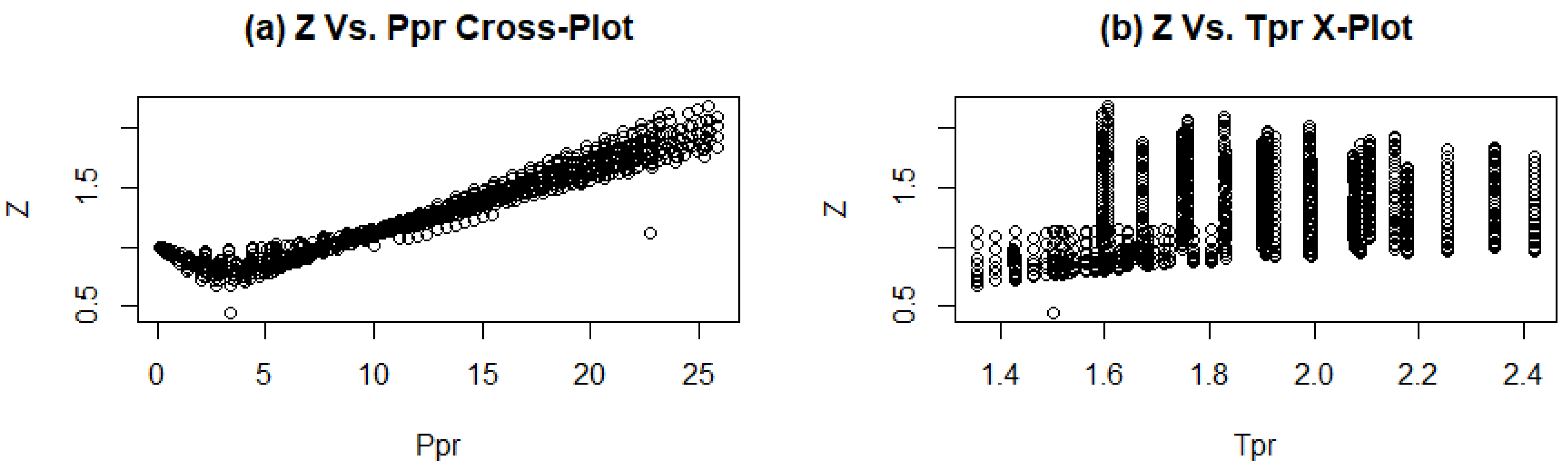
3.2. Data Exploration

The gathered data were explored by calculating the statistical properties, such as the mean, standard deviation, and range. This step is important to assess the data quality and check whether there are any outliers and how to handle them. The next step is to visualize the relationship between the Z-factor and each of the (P_pr) and (T_pr), which is essential to decide whether the exploratory variables can be used to directly predict the Z-factor or whether they need to be transformed into new variables to facilitate the model selection process.

Based on data exploration and visualization, the Z-factor was found to be difficult to predict directly from the (P_pr) and (T_pr). Accordingly, variable transformation is needed to recognize the hidden patterns in the relationship between the Z-factor and each of the (P_pr) and (T_pr). One of the common ways to transform variables is to combine different variables together. Accordingly, the ratio (X) was obtained by dividing the P_pr by the T_pr.

Another pre-modeling step is to normalize the variables by subtracting each variable’s observation from the mean and dividing the result by the standard deviation. This process is called “Centering and Scaling”. It can be performed by using the “scale” function of the “base” package in R [35]. This step is vital to enhance the stability of the model to be postulated [36,37,38].

3.3. Model Selection

The relationship between the Z-factor and (X) was found to be curvilinear. Therefore, a quadratic regression model was thought to be more appropriate than a linear model. In order to prove this, the “lm” function in R was used to compare the linear and quadratic cases. The comparison criteria between the linear and quadratic models, were the R-squared value and standard error. Moreover, the residuals were compared quantitatively and plotted in order to determine which model would be more representative of the data. Finally, it was proven that a quadratic model should be selected.

As the linearity between the Z-factor and X is not particularly high, another model is needed to better estimate the Z-factor based on machine learning. Recently, neural networks have been widely used to solve non-linear problems due to their advantages over regression models [39,40]. Neural networks are among the supervised-learning tools that provide a function based on a network of input(s) and output(s) [41]. Therefore, a neural network is expected to be more accurate than the regression model.

In this study, the multi-layer-feedforward neural network (MLFN) was selected as it is widely used for general-purpose non-linear regression models and due to its ability to extract hidden patterns from data. Another advantage of the MLFN is that it can perform input–output mapping by modifying the weights of the coefficients until reaching the least difference between the desired output and the network’s actual output [42].

3.4. Model Postulation

Statistical Regression Modeling

Based on the Z–X relationship, the model is expected to follow the quadratic formula:

$$\mathrm{Z}={\beta }_1{\mathrm{X}}^2+{\beta }_2\mathrm{X}+{\beta }_3$$

(8)

where Z is the output (response) variable, X is the P_r-over-T_r ratio (explanatory variable), and the coefficients of the equations are ${\beta }_1$, ${\beta }_2$, and ${\beta }_3$. Given the observations of the Z-factor and X, the models’ coefficients can be obtained, based on the Bayes’ theorem [43], from the joint distribution of the likelihood and priors, as shown below:

$$\mathrm{P}\left(\beta |\mathrm{y}\right)=\frac{\mathrm{P}\left(\mathrm{y}|\beta \right)\mathrm{P}\left(\beta \right)}{\mathrm{P}\left(\mathrm{y}\right)}$$

where P($\beta$|y) is the posterior probability of the coefficients’ vector ($\beta$) given the likelihood (y), which represents the actual observations, the expression “P(y|$\beta$)P($\beta$)” is the joint distribution of the likelihood and the priors of the coefficients, while P(y) is the marginal distribution of the likelihood (y). Therefore, the posterior probability is equivalent to the joint distribution of the likelihood and priors, as shown below:

$$\mathrm{P}\left(\beta |\mathrm{y}\right) \alpha {\displaystyle \int }\mathrm{P}\left(\mathrm{y}|\beta \right)\mathrm{P}\left(\beta \right)d\beta$$

In some cases, the joint probability of the model is too complex to be integrated. That’s why the Markov chain Monte Carlo (MCMC) simulation can be used to obtain the posterior distribution of such models [44]. A Markov chain (MC) is a chain of numbers in which each number depends on the previous number in the sequence. If {$x_1, x_2, x_3$, …, $x_{\mathrm{t}}$} is a Markov chain, where {1, 2, 3, …, t} are successive points in time, the probability of the variables can be expressed according to the chain role, as shown below:

$$\mathrm{P}\left(x_1, x_2, x_3, \dots , x_{\mathrm{t}}\right)=\mathrm{P}\left(x_1\right) \mathrm{P}(x_2|x_1) \mathrm{P}(x_3|x_2,x_1), \dots , \mathrm{P}(x_{\mathrm{t}}|x_{\mathrm{t}-1}, x_{\mathrm{t}-2}, \dots , x_2,x_1)$$

Assuming that the transition probabilities are not time-dependent, the probability at the time (t) depends only on the value of {$x_{\mathrm{t}-1}$}:

$$\mathrm{P}\left(x_1, x_2, x_3, \dots x_n\right)=\mathrm{P}\left(x_1\right) \mathrm{P}(x_2|x_1) \mathrm{P}(x_3|x_2), \dots , \mathrm{P}(x_{\mathrm{t}}|x_{\mathrm{t}-1})$$

The stationary distribution of the MC is the initial distribution at which the transition probability does not change in any given state. The aim of the MCMC is to draw multiple random values from a proposed distribution so that the sequence of all simulations is a Markov chain, and the stationary distribution of that chain is the posterior distribution. According to the law of large numbers [45], the MC should converge to the true mean of the posterior distribution that can be assigned to the coefficient. Therefore, each coefficient in the model is obtained by calculating the posterior mean of all the realizations drawn from the proposed distribution.

The aim of the statistical regression model is to fit a linear relationship between the Z-factor, which is the response variable, and each of the squared-X and X, which are the explanatory variables of the model. Accordingly, the likelihood function of the model can be expressed as shown below:

$$Z|\beta ,{{\mathrm{X}}^2}_{\mathrm{i}}, {\mathrm{X}}_{\mathrm{i}}, {\sigma }^2 ~ \mathrm{N}\left({\beta }^1{\mathrm{X}}^2+{\beta }^2\mathrm{X}+{\beta }^3,{\mathsf{\sigma }}^2\right)$$

Given the coefficients’ vector, the explanatory variables ${\mathrm{X}}^2$, and the variance σ², the Z-factor follows a normal distribution. The mean of this distribution equals the linear expression of the covariates and coefficients. The symbol (i) is the observations’ index.

The next layer of the model consists of the coefficients’ vector $\mathsf{\beta }$ and the variance σ², which are considered the priors of the model. In order to determine an idea as to the probability distribution function of each of the coefficients, the “lm” function of the “stats” package [39] was used, in R, to fit a preliminary linear model that resulted in the hyper-parameters (mean and standard deviation) of each coefficient. Accordingly, the prior functions of the three coefficients can be expressed as follows:

$${\beta }_{\mathrm{j}}~ \mathrm{N}\left({\mu }_{\mathrm{j}},{\tau }_{\mathrm{j}}\right), \mathrm{j}=\left\{1,2,3\right\}$$

where the coefficient β_j is normally distributed with a mean $\mu$_j and standard deviation $\tau$_j. The variance of the model follows an inverse-gamma distribution, which is a type of continuous probability distribution [46] that is always positive and depends on two parameters: the shape parameter α and the scale parameter β. The inverse-gamma is used to draw the unknown variance of a normal distribution, where the priors are uninformative. Therefore, the variance (${\mathsf{\sigma }}^2$) is given by:

$${\mathsf{\sigma }}^2 ~ \mathrm{IG}\left(\alpha ,\beta \right)$$

where α and β are the priors of the variance ${\mathsf{\sigma }}^2$. The hyper-parameters of the variance’s distribution were treated as non-informative priors. The values of the α and β were assumed to be greater than 1 to include high random-error values.

The aim of the model is to use the MCMC simulation to randomly draw multiple realizations of the coefficients from their common distribution and, then, to calculate the Z-factor by substituting the posterior means of the coefficients to Equation (8). The graphical representation of the statistical model is shown in Figure 1, where: Z_i is the response variable of an observation (i); X²_i and X_i are the explanatory factors; i is the observations’ index, which ranges from 1 to n; b_j is the coefficients vector, which depends on the mean µ and standard deviation τ; and σ² is the variance of the model, which depends on the shape parameter α and scale parameter β. The statistical model was postulated and trained in R using the “rjags” package, which uses the MCMC to generate a sequence of dependent samples from the posterior distribution of the parameters [47,48].

3.5. MLFN Model

Recently, neural networks have been widely used to solve non-linear problems due to their advantages over regression models [39,40]. One of the common neural networks is the multi-layer feedforward (MLFN) neural network, which consists of three main types of layers: an input layer, one or more hidden layers, and an output layer [49]. The advantage of this network is that hidden layers enable it to estimate variables based on non-linear relationships.

The MLFN layers are fully connected, so that all units in one layer are connected to all units in the next layer [49]. Each connection is controlled by a random weight that should be adjusted by an algorithm, such as the backpropagation method [50], until the optimum set of weights is obtained, so that the predicted output best matches the actual output. The aim of this algorithm is to feed the hidden layer(s) with the input units associated with their weights and, then, to produce a function to calculate the output from the weighted sums of the inputs.

The structure of the MLFN in the current study consists of three layers: an input layer, three hidden layers, and an output layer. The input layer consists of two neurons, which are X and X², while the output layer consists of one neuron, which is the Z-factor. The number of neurons in the hidden layer is adjusted until the best performance is achieved. The network was postulated and trained using the “neural net” package in R, which calculates the generalized weights [51] and provides customized settings for error and activation function.

Eventually, the statistical and MLFN models were compared based on the correlation coefficient and residual analysis. The correlation coefficient was obtained using the “cor.test” function of the “stats” package in R based on Pearson’s product moment correlation coefficient [52]. The residual analysis was performed by plotting the residuals to show how far the residuals were from the zero line [53].

4. Results

4.1. Data Gathering

The collected data from different sources in the literature included about 1079 data points for each of the Z-factor, P_pr, and T_pr to achieve the goal of this study. The statistical distribution of the data points, such as the minimum (Min), maximum (Max), mean and standard deviation (Std), are reported in

Table 1. Data statistics before cleaning.

Statistical Property	Ppr	Tpr	Z
Count	1079	1079	1079
Mean	12.360625	1.838588	1.285249
Std	6.900794	0.253642	0.351064
Min	0.162203	1.357125	0.445000
Max	25.821442	2.420676	2.192700

.

4.2. Data Exploration

It is clear that the minimum and maximum Z values of the data points were far from the mean. In addition, the Z-P_pr and Z-T_pr scatter plots (Figure 2a,b, respectively) show some residuals. Accordingly, the residuals were removed to avoid high variance in the data.

Another observation is that the P_pr values were far from those of the Z-factor and T_pr, as shown in the box plots in Figure 3. This is why each variable was normalized by centering and scaling.

The relationship between the Z-factor and each of the P_pr and T_pr seemed non-linear and showed a high degree of randomness. In addition, there were some residuals that were far away from the data range. Therefore, the data should be cleaned and the variables transformed in order to be ready for modeling.

It is obvious how the Z–X relationship (Figure 4) was more meaningful and less noisy than the Z–P_pr and Z–T_pr relationships (Figure 2a,b, respectively). The next step was to postulate a model that could estimate the Z-factor from the X. Two methods were applied to do so: statistical regression and multi-layer feedforward neural network (MLFN).

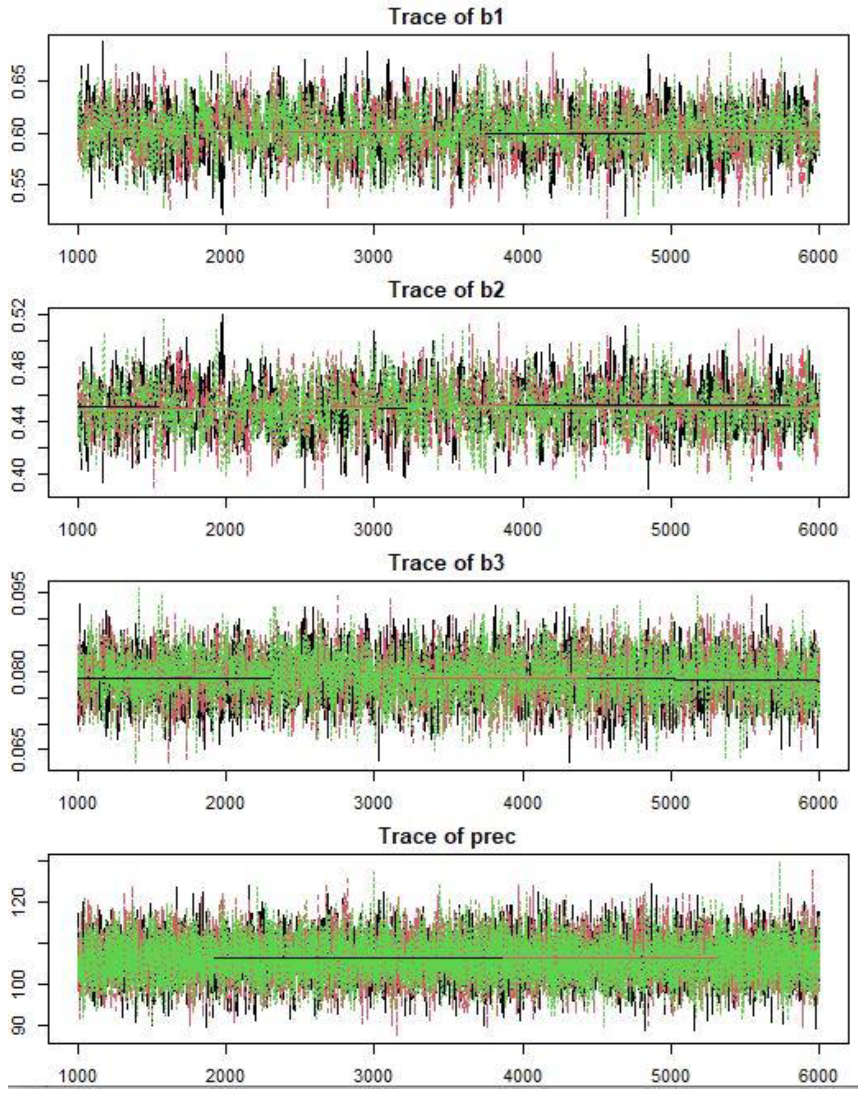
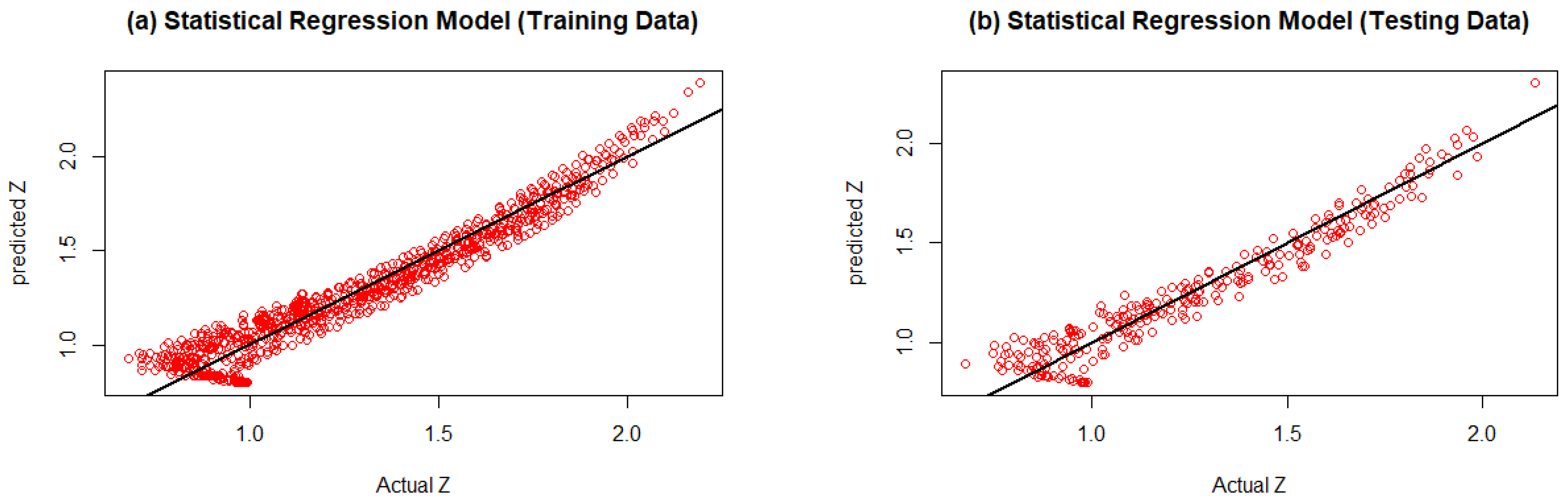
4.3. Results of the Statistical Regression Model

The data points were divided into training and testing points with the percentages 75% and 25%, respectively. Figure 5 shows the trace-plots of the Markov chains, which aim to estimate the models’ coefficients and precision (prec), which is the reciprocal of the variance. The number of iterations is shown on the X-axis and the value of each coefficient is shown on the Y-axis.

Each parameter was simulated by using three chains, and was expected to converge at the mean value of its multiple realizations. The chains reached the stationary distribution at a number of iterations that ranged from 1500 to 2000. The mean values of the three coefficients (β₁, β₂, and β₃) were 0.6, 0.45, and 0.08, respectively. When applying these values to Equation (8), the following equation is obtained:

$$\mathrm{Z}=0.6 {\mathrm{X}}^2+0.45 \mathrm{X}+0.08$$

After un-scaling the predicted and actual values of the Z-factor for both the training and testing data, the correlation coefficient was calculated using the “cor.test” function of the “stats” package in R. Figure 6a,b show the predicted-versus-actual plots for the training and testing data, resulting in the correlation-coefficient values 0.969 and 0.967, respectively. The plots show a positive correlation between the predicted and actual values. However, there are some residuals in the bottom-left of the plot.

4.4. Results of the MLFN Model

The graphical representation of the MLFN model is shown in Figure 7, where the network consists of an input layer with two nodes (green circles), three hidden layers (black circles), and an output layer (blue circle). The number of hidden layers and the number of nodes in each of them was adjusted until reaching the least mean-square error (MSE). The best network performance was reached after 2011 steps by using 2, 5, and 2 nodes in the hidden layers, resulting in an MSE value equal to 0.461. The network was applied to the data, resulting in a strong positive correlation between the predicted and actual Z-factor, as shown in Figure 8, for the training and testing data, respectively. The correlation coefficient of the training and testing data were 0.982 and 0.979, respectively.

5. Discussion

The purpose of engaging both the statistical and MLFN models in this study was to use the regression model as a pre-modeling step for the neural network. In other words, it is important to use statistical models to recognize the hidden patterns in data and test various sets of model variables in order to obtain the best group of predictors that could be later used as inputs to neural networks. Another benefit of combining statistical models and neural networks is that it shows how machine-learning could overcome the randomness inside data and recognize the patterns hidden in them. This is clear when comparing the actual-predicted Z-factor plots of the statistical and MLFN models, as shown in Figure 5 and Figure 8, respectively, where the MLFN model shows stronger linearity and less residuals relative to the statistical model. This hypothesis is evidenced by the correlation-coefficient values, which were higher in MLFN compared to the regression model, as shown in

Table 2. The correlation-coefficient values of the training and testing data for the statistical and MLFN models.

Model Name	Training Data	Testing Data
Statistical Model	0.969	0.967
MLFN Model	0.982	0.979

.

Both models showed a high degree of stability because the correlation-coefficient values of the training and testing data were so close to each other, which indicates that there was no over-fitting. However, a more precise comparison was drawn between the two models by using the residual analysis shown in Figure 9a,b, where the residuals of the statistical and MLFN models are plotted, respectively. Unlike the statistical model, the MLFN model showed residuals that were closer to the zero red line and more centered around it. This is how the MLFN model improved the Z-factor prediction by using the power of machine learning.

6. Conclusions

The gas compressibility factors of natural gases were calculated using a multi-layer-feedforward neural network and statistical regression as a function of the ratio of the pseudo-reduced pressure (P_pr) and the pseudo-reduced temperature (T_pr). The models were postulated and trained based on the data from 1077 samples obtained from the literature.

• The P_pr and T_pr were calculated using the compositional analysis and the reservoir pressure and temperature for each sample, according to Kay’s rule.
• The statistical regression model and the MLFN neural network were postulated and trained for a wide range of P_pr (0.12 to 25.8) and T_pr (1.3 to 2.4).
• The designed MLFN neural network consists of one input layer with two anodes, three hidden layers, and one output layer.
• Both the correlation coefficient and the residual analysis showed that the MLFN model is more stable and accurate than the statistical model. However, statistical modeling is an important step before running neural networks because it helps recognize the hidden patterns in data and test various sets of model variables in order to obtain the best group of predictors that could be later used as inputs to neural networks.

It can be noted that the use of MLFN neural networks is an important, advantageous, and cheap technique to calculate the gas compressibility of natural gases.

References

1. Gaganis, V.; Homouz, D.; Maalouf, M.; Khoury, N.; Polychronopoulou, K. An Efficient Method to Predict Compressibility Factor of Natural Gas Streams. Energies 2019, 12, 2577. [Google Scholar] [CrossRef] [Green Version]
2. Cengel, Y.A.; Boles, M.A. Energy, energy transfer, and general energy analysis. In An Engineering Approach; McGraw-Hill: New York, NY, USA, 2007. [Google Scholar]
3. Danesh, A. PVT and Phase Behaviour of Petroleum Reservoir Fluids; Elsevier: Amsterdam, The Netherlands, 1998. [Google Scholar]
4. Sanjari, E.; Lay, E.N. Estimation of natural gas compressibility factors using artificial neural network approach. J. Nat. Gas Sci. Eng. 2012, 9, 220–226. [Google Scholar] [CrossRef]
5. Azizi, N.; Behbahani, R.M. Predicting the compressibility factor of natural gas. Pet. Sci. Technol. 2017, 35, 696–702. [Google Scholar] [CrossRef]
6. Mohamadi-Baghmolaei, M.; Azin, R.; Osfouri, S.; Mohamadi-Baghmolaei, R.; Zarei, Z. Prediction of gas compressibility factor using intelligent models. Nat. Gas Ind. B 2015, 2, 283–294. [Google Scholar] [CrossRef] [Green Version]
7. Almehaideb, R.A.; Al-Khanbashi, A.S.; Abdulkarim, M.; Ali, M.A. EOS tuning to model full field crude oil properties using multiple well fluid PVT analysis. J. Pet. Sci. Eng. 2000, 26, 291–300. [Google Scholar] [CrossRef]
8. Varzandeh, F.; Stenby, E.H.; Yan, W. Comparison of GERG-2008 and simpler EoS models in calculation of phase equilibrium and physical properties of natural gas related systems. Fluid Phase Equilibria 2017, 434, 21–43. [Google Scholar] [CrossRef] [Green Version]
9. Hendriks, E.; Kontogeorgis, G.; Dohrn, R.; De Hemptinne, J.-C.; Economou, I.; Žilnik, L.F.; Vesovic, V. Industrial Requirements for Thermodynamics and Transport Properties. Ind. Eng. Chem. Res. 2010, 49, 11131–11141. [Google Scholar] [CrossRef]
10. Orbey, H.; Sandler, S.I. Modeling Vapor-Liquid Equilibria: Cubic Equations of State and Their Mixing Rules; Cambridge University Press: Cambridge, UK, 1998. [Google Scholar]
11. Dindoruk, B.; Ratnakar, R.R.; He, J. Review of recent advances in petroleum fluid properties and their representation. J. Nat. Gas Sci. Eng. 2020, 83, 103541. [Google Scholar] [CrossRef]
12. Seitmaganbetov, N.; Rezaei, N.; Shafiei, A. Characterization of crude oils and asphaltenes using the PC-SAFT EoS: A systematic review. Fuel 2021, 291, 120180. [Google Scholar] [CrossRef]
13. Fayazi, A.; Arabloo, M.; Mohammadi, A.H. Efficient estimation of natural gas compressibility factor using a rigorous method. J. Nat. Gas Sci. Eng. 2014, 16, 8–17. [Google Scholar] [CrossRef]
14. Al-Fatlawi, O.; Hossain, M.; Osborne, J. Determination of best possible correlation for gas compressibility factor to accurately predict the initial gas reserves in gas-hydrocarbon reservoirs. Int. J. Hydrogen Energy 2017, 42, 25492–25508. [Google Scholar] [CrossRef]
15. Brill, J.; Beggs, H. Two-Phase Flow in Pipes; INTERCOMP Course, The Hague. University of Tulsa: Tulsa, OK, USA, 1974. Available online: https://www.scribd.com/doc/311112901/Brill-J-P-Beggs-H-D-Two-Phase-Flow-in-Pipes (accessed on 26 December 2021).
16. Kamyab, M.; Sampaio, J.H.; Qanbari, F.; Eustes, A.W. Using artificial neural networks to estimate the z-factor for natural hydrocarbon gases. J. Pet. Sci. Eng. 2010, 73, 248–257. [Google Scholar] [CrossRef]
17. Dranchuk, P.; Abou-Kassem, H. Calculation of Z Factors for Natural Gases Using Equations of State. J. Can. Pet. Technol. 1975, 14, PETSOC-75-03-03. [Google Scholar] [CrossRef]
18. Fatoorehchi, H.; Abolghasemi, H.; Rach, R.; Assar, M. An improved algorithm for calculation of the natural gas compressibility factor via the Hall-Yarborough equation of state. Can. J. Chem. Eng. 2014, 92, 2211–2217. [Google Scholar] [CrossRef]
19. Kumar, N.A. Compressibility Factors for Natural and Sour Reservoir Gases by Correlations and Cubic Equations of State. Ph.D. Thesis, Texas Tech University, Lubbock, TX, USA, 2004. [Google Scholar]
20. Azizi, N.; Behbahani, R.; Isazadeh, M. An efficient correlation for calculating compressibility factor of natural gases. J. Nat. Gas Chem. 2010, 19, 642–645. [Google Scholar] [CrossRef]
21. Omobolanle, O.C.; Akinsete, O.O. A Comprehensive Review of Recent Advances in the Estimation of Natural Gas Compressibility Factor. In Proceedings of the SPE Nigeria Annual International Conference and Exhibition, Lagos, Nigeria, 2–4 August 2021. [Google Scholar]
22. Tariq, Z.; Aljawad, M.S.; Hasan, A.; Murtaza, M.; Mohammed, E.; El-Husseiny, A.; Alarifi, S.A.; Mahmoud, M.; Abdulraheem, A. A systematic review of data science and machine learning applications to the oil and gas industry. J. Pet. Explor. Prod. Technol. 2021, 11, 4339–4374. [Google Scholar] [CrossRef]
23. Normandin, A.; Grandjean, B.P.A.; Thibault, J. PVT data analysis using neural network models. Ind. Eng. Chem. Res. 1993, 32, 970–975. [Google Scholar] [CrossRef]
24. Chamkalani, A.; Mae’Soumi, A.; Sameni, A. An intelligent approach for optimal prediction of gas deviation factor using particle swarm optimization and genetic algorithm. J. Nat. Gas Sci. Eng. 2013, 14, 132–143. [Google Scholar] [CrossRef]
25. Azizi, N.; Rezakazemi, M.; Zarei, M.M. An intelligent approach to predict gas compressibility factor using neural network model. Neural Comput. Appl. 2017, 31, 55–64. [Google Scholar] [CrossRef]
26. Saemi, M.; Ahmadi, M.; Varjani, A.Y. Design of neural networks using genetic algorithm for the permeability estimation of the reservoir. J. Pet. Sci. Eng. 2007, 59, 97–105. [Google Scholar] [CrossRef]
27. Moghadassi, A.R.; Parvizian, F.; Hosseini, S.M.; Fazlali, A.R. A new approach for estimation of PVT properties of pure gases based on artificial neural network model. Braz. J. Chem. Eng. 2009, 26, 199–206. [Google Scholar] [CrossRef] [Green Version]
28. Saghafi, H.; Arabloo, M. Development of genetic programming (GP) models for gas condensate compressibility factor determination below dew point pressure. J. Pet. Sci. Eng. 2018, 171, 890–904. [Google Scholar] [CrossRef]
29. Buxton, T.S.; Campbell, J.M. Compressibility Factors for Lean Natural Gas-Carbon Dioxide Mixtures at High Pressure. Soc. Pet. Eng. J. 1967, 7, 80–86. [Google Scholar] [CrossRef]
30. Satter, A.; Campbell, J.M. Non-Ideal Behavior of Gases and Their Mixtures. Soc. Pet. Eng. J. 1963, 3, 333–347. [Google Scholar] [CrossRef] [Green Version]
31. McLeod, W.R. Applications of Molecular Refraction to the Principle of Corresponding States; The University of Oklahoma: Norman, OK, USA, 1968. [Google Scholar]
32. Liu, H.; Sun, C.-Y.; Yan, K.-L.; Ma, Q.-L.; Wang, J.; Chen, G.-J.; Xiao, X.-J.; Wang, H.-Y.; Zheng, X.-T.; Li, S. Phase behavior and compressibility factor of two China gas condensate samples at pressures up to 95MPa. Fluid Phase Equilibria 2013, 337, 363–369. [Google Scholar] [CrossRef]
33. Li, Q.; Guo, T.-M. A study on the super-compressibility and compressibility factors of natural gas mixtures. J. Pet. Sci. Eng. 1991, 6, 235–247. [Google Scholar] [CrossRef]
34. Sun, C.-Y.; Liu, H.; Yan, K.-L.; Ma, Q.-L.; Liu, B.; Chen, G.-J.; Xiao, X.-J.; Wang, H.-Y.; Zheng, X.-T.; Li, S. Experiments and Modeling of Volumetric Properties and Phase Behavior for Condensate Gas under Ultra-High-Pressure Conditions. Ind. Eng. Chem. Res. 2012, 51, 6916–6925. [Google Scholar] [CrossRef]
35. Becker, R.A.; Chambers, J.M.; Wilks, A.R. The New S Language; Wadsworth & Brooks/Cole: Pacific Grove, CA, USA, 1988. [Google Scholar]
36. Geladi, P.; Kowalski, B. Partial Least Squares Regression: A Tutorial. Anal. Chim. Acta 1986, 185, 1–17. [Google Scholar] [CrossRef]
37. Jolliffe, I.T. Principla Component Analysis, 2nd ed.; Springer: New York, NY, USA, 2002. [Google Scholar]
38. Mulaik, S.A. Foundations of Factor Analysis, 2nd ed.; Chapman Hall/CRC: London, UK, 2009. [Google Scholar]
39. Friedman, J.H. The Elements of Statistical Learning: Data Mining, Inference, and Prediction; Springer Open: Berlin/Heidelberg, Germany, 2017. [Google Scholar]
40. Hami-Eddine, K.; Klein, P.; Richard, L. Well facies based supervised classification of prestack seismic: Application to a turbidite field. In Proceedings of the 2009 SEG Annual Meeting, Houston, TX, USA, 25–30 October 2009. [Google Scholar]
41. Nikravesh, M.; Zadeh, L.A.; Aminzadeh, F. Soft Computing and Intelligent Data Analysis in Oil Exploration; Elsevier: Amsterdam, The Netherlands, 2003. [Google Scholar]
42. Svozil, D.; Kvasnicka, V.; Pospichal, J. Introduction to multi-layer feed-forward neural networks. Chemom. Intell. Lab. Syst. 1997, 39, 43–62. [Google Scholar] [CrossRef]
43. Stuart, A. Kendall’s Advanced Theory of Statistics; Distribution Theory; Wiley: Hoboken, NJ, USA, 1994; Volume 1. [Google Scholar]
44. Banerjee, S.; Carlin, B.P.; Gelfand, A.E. Hierarchical Modeling and Analysis for Spatial Data; Chapman: London, UK, 2003; Hall/CRC: Boca Raton, FL, USA, 2003. [Google Scholar]
45. Gao, R.; Sheng, Y. Law of large numbers for uncertain random variables with different chance distributions. J. Intell. Fuzzy Syst. 2016, 31, 1227–1234. [Google Scholar] [CrossRef] [Green Version]
46. Abid, S.H.; Al-Hassany, S. On the inverted gamma distribution. Int. J. Syst. Sci. Appl. Math. 2016, 1, 16–22. [Google Scholar]
47. Lunn, D.; Spiegelhalter, D.; Thomas, A.; Best, N. The BUGS project: Evolution, critique and future directions. Stat. Med. 2009, 28, 3049–3067. [Google Scholar] [CrossRef] [PubMed]
48. Plummer, M.; Best, N.; Cowles, K.; Vines, K. CODA: Convergence Diagnosis and Output Analysis for MCMC. R News 2006, 6, 7–11. [Google Scholar]
49. Rumelhart, D.E.; Hinton, G.E.; Williams, R.J. Learning representations by back-propagating errors. Nature 1986, 323, 533–536. [Google Scholar] [CrossRef]
50. Werbos, P.J. The Roots of Backpropagation: From Ordered Derivatives to Neural Networks and Political Forecasting; John Wiley & Sons: Hoboken, NJ, USA, 1994; Volume 1. [Google Scholar]
51. Intrator, O.; Intrator, N. Using Neural Nets for Interpretation of Nonlinear Models. In Proceedings of the Statistical Computing Section; American Statistical Society: San Francisco, CA, USA, 1993; pp. 244–249. [Google Scholar]
52. Gooch, J.W. Pearson’s Product-Moment Correlation Coefficient. In Encyclopedic Dictionary of Polymers; Springer Science and Business Media LLC: Berlin/Heidelberg, Germany, 2011; p. 991. [Google Scholar]
53. Chambers, J.; Hastie, T. Chapter 4 of Statistical Models in S. In Linear Models; Wadsworth & Brooks/Cole: Pacific Grove, CA, USA, 1992. [Google Scholar]
Scheme 1. The graphical representation of the statistical model.
Energies 15 01807 sch001
Figure 1. The graphical representation of the statistical model.
Energies 15 01807 g001
Figure 2. Cross plots of (a) Z vs. Ppr and (b) Z vs. Tpr.
Energies 15 01807 g002
Figure 3. Box plots of the range values of Ppr, Tpr, and Z factor.
Energies 15 01807 g003
Figure 4. Cross plots of Z vs. X.
Energies 15 01807 g004
Figure 5. The trace-plots of the Markov chains that simulate the statistical model’s coefficients (β1, β2, and β3) and the precision (prec).
Energies 15 01807 g005
Figure 6. Plots of predicted Z-factor vs. actual Z-factor for the statistical models of both the training and testing data.
Energies 15 01807 g006
Figure 7. The graphical representation of the MLFN model.
Energies 15 01807 g007
Figure 8. Plots of predicted Z-factor vs. actual Z-factor for the MLFN model of both the training and testing data.
Energies 15 01807 g008
Figure 9. The residual plots of the (a) statistical and (b) MLFN models.
Energies 15 01807 g009