Abstract
The paper presents a comparative analysis of selected algorithms for prediction and data analysis. The research was based on data taken from a computerized numerical control (CNC) milling machine. Methods of knowledge extraction from very large datasets, characteristics of classical analytical methods used in datasets and knowledge discovery in database (KDD) processes were also described. The aim of the study is a comparative analysis of selected algorithms for prediction and data analysis to determine the time and degree of tool usage in order to react early enough and avoid unwanted incidents affecting production effectiveness. The research was based on K-nearest neighbor, decision tree and linear regression algorithms. The influence of the rate of learning and testing set sizes were evaluated, which may have an important impact on the optimization of the time and quality of computation. It was shown that precision decreases with the increase of the K value of the average group, while the percentage of the number of classes in a given set (recall) increases. The harmonic mean for the group mean also increases with increasing K, while a significant decrease in these values was observed for the standard deviations of the group. The numerical value of accuracy decreases with increasing K.
1. Introduction
Tool health condition monitoring is of great interest to researchers in the era of IoT and Industry 4.0 development. The interest in tool condition monitoring stems from the fact that we are trying to make production unmanned. This is possible only if we provide an appropriate method of monitoring tool wear and tool damage detection. In the course of the production process, the tool is subject to wear, which has a direct effect on the surface quality of the workpieces. In addition, damage to the tool during the production process can lead to damage to the entire machine, resulting in significant costs and production downtime. It is therefore important to prevent damage to the tool in this context, based on the symptoms shown by the measured signals as the tool wear increases and to catch the direct moment of irreversible damage relatively early in order to prevent it. Currently, tool replacement is based on conservative estimates of tool life derived from documentation provided by the manufacturer. Such solutions are not optimal because they involve too many changes, as the full tool life is not taken into account, and thus valuable production time is lost.
The research aims to determine the time and degree of tool wear in order to react early enough and avoid unwanted incidents affecting production optimization based on advanced data extraction methods. Industry 4.0 enforces the use of an online tool condition monitoring (TCM) system, which will ensure better health of the process and especially the cutting tool by continuously monitoring specific parameters.
Tool condition monitoring techniques include direct and indirect measurements of tool wear. Direct measurement of the cutting edge provides the most accurate information about the physical deterioration of the cutting tool. The cutting edge is an essential component in the metal removal process. During the continuous machining process, the performance of the cutting tool deteriorates due to tool wear or even tool breakage. Tool failure reduces the machining quality and even affects the dimensional change of the product. Direct methods are based on direct measurements of tool wear, e.g., optical methods, electrical resistivity or vision systems, etc. These methods are characterized by high accuracy but have the disadvantages of high costs and technical complexity of the solutions. Indirect methods are based on the relationship between tool conditions and measurable signals from machining processes. Such signals include contact force, vibration, acoustic waves or cutting temperature. Tool states are then diagnosed using these extracted features and artificial intelligence techniques. The correct interpretation and analysis of the parameter values make it possible to detect tool wear. The problem is an improved interpretation of signals, which are generally considered to be stochastic and non-stationary rather than deterministic, and also because there is a non-linear relationship between measured features and tool wear.
For thousands of years, people have been interested in algorithms and applied them manually. However, this approach is very time-consuming and requires a lot of attention. Thanks to algorithms, one can find solutions, and the faster and easier it is to find a solution, the better. There is a large discrepancy between algorithms proposed by historical geniuses (Euclid, Newton, Gauss) and modern algorithms developed by scientists teaching at universities or working in research laboratories. The main reason for such large gaps is the use of the computer. Without hesitation, one can say that thanks to computers, one can solve a given problem much faster with the use of algorithms. The continuous development of new algorithms has been happening very rapidly since the emergence of large and powerful computer systems. In addition, the constantly increasing power of computers is due to the fact that their computing power is inexpensive. Thus, the ubiquity of computers contributes to better, faster and more efficient ways of solving problems using algorithms.
Therefore, in order to effectively utilize the existing machining process data of similar tools and features, this paper proposes an effective data exploration approach to reveal the relationship between machining features and machining operations. The presented study aims to evaluate the performance of a classifier in the milling process, which can be used to develop an online TCM system. Selected methods for knowledge extraction from very large datasets were analyzed in detail. The research was based on K-nearest neighbor, decision tree and linear regression algorithms. The effect of the rate of the learning and testing set size was evaluated. The aim was to obtain an effective and efficient classifier with minimum response time in the design of the process TCM system. An attempt was made to use histogram features extracted from vibration signals, and a decision tree was used to select the most relevant features from the set of extracted features.
In order to verify the effectiveness of the proposed approach, various methods, i.e., K-nearest neighbors, decision tree and linear regression, were used for data analysis and prediction. In addition, the effect of different proportions of configurations of learning and test sets affecting the data mining process and resource optimization was studied. The rest of the paper is organized as follows. Section 2 references work on available studies on data mining and implementations of real-time intelligent milling diagnostic systems. Section 3 shows the mathematical background concerning the research methodology, analyzed data structure and estimation of the main statistical characteristics of the obtained results using the Python environment. In Section 4, the detailed results of the analysis are presented, which concerns the ratio of the test and learning set size of the used models on the efficient classification methods used in real-time intelligent milling diagnostic systems and its impact on optimization of the time and quality of computation. The work ends with a summary of the obtained research results and conclusions.
2. Literature Review
Algorithms represent a sequence of steps, and their scope is incredibly large. Some algorithms have applications in areas of real-life—science, medicine, finance, communication, logistics or industrial production [1]. The efficient processing of algorithms is in large part dependent on the correct coding of the computational process, using the computational environment as well as the programming language itself. As shown in [2], the same algorithmic problem coded in different programming languages and run in different execution environments with the same hardware parameters of the computing machine (in terms of execution time) differed greatly in these variants. The computational complexity of a particular mathematical and computational problem also directly depends on the used data structures. Currently, we observe an exponential growth of data to be analyzed, for which it was necessary to develop new data structures as well as the algorithms of data analysis and extraction. For several years now, the term “big data” has become synonymous with this situation.
In recent years, the term Industry 4.0 has gained a lot of popularity. Generally speaking, Industry 4.0 is a concept that aims to automate production by digitizing industrial processes and applying smart technologies, such as Internet of Things (IoT) devices. Industry 4.0 solutions extend beyond smart factory applications to include logistics and traceability, smart agriculture, healthcare and other sectors. The vast amount of data generated presents challenges in collecting and managing big data, but also creates a number of opportunities, such as extracting insights from that data, which can drive decision-making and continuous improvement of industrial operations and production chain processes. According to [3], the authors note that the vastness of data generated by sensors in big data analytics (BDA) is becoming one of the main pillars of Industry 4.0. The concept of big data and big data analytics has become a promising tool to support the competitive advantage of companies by enhancing data-driven performance. The authors confirm that BDA and innovation can improve the performance of companies, leading to competitive advantages.
Data collection and the concept of big data are justified in ensuring the continuous and reliable operation of the equipment of the modern factory 4.0. The presence of many wireless sensors monitoring the parameters of, e.g., CNC machines, leads to the generation of terabytes of data that need to be efficiently analyzed, often in real-time, and decisions made based on them. In [4], a hybrid component-based fault detection and diagnosis (FDD) approach for industrial sensor systems is established and analyzed to provide a hybrid scheme that combines the advantages and eliminates the disadvantages of both model-based and data-driven diagnosis methods.
Online data analysis does not guarantee the avoidance of costly failures or fault tolerance. Predictive, anticipatory action is required. Hence, it becomes necessary to use artificial intelligence algorithms for advanced data mining, including predicting future data and discovering hidden patterns based on data collected in big data systems. As shown in [5], predictive maintenance (PdM) has the potential to reduce industrial costs by predicting failures and increasing component uptime. Currently, factories monitor their assets, and most of the collected data relate to correct operating conditions. Therefore, semi-supervised data-driven models are important to enable PdM by learning from asset data. However, their main challenges in industrial applications are to achieve high accuracy in anomaly detection, diagnosis of new failures and adaptability to changing environmental and operational conditions (EOC).
In [6,7], the authors propose the use of fractal and multifractal analysis mechanisms, which can help to discover the structure of the communication system, especially the traffic pattern and characteristics, in order to better understand the threats and detect anomalies in the network performance. In particular, the authors’ work presents the use of fractal analysis in detecting threats and anomalies. Based on data collected from monitoring and devices, the response to the incident was analyzed, and multifractal network traffic spectra were created before and during the incident. The collected information allows for verifying the thesis and confirming the effectiveness of multifractal methods in detecting anomalies in the operation of any information and communication technology (ICT) network. Such solutions will contribute to the development of advanced intrusion detection systems.
This approach to PdM can be applied in other areas. The authors in [8] show that increasing renewable energy leads to increasingly volatile and rising electricity prices. This poses a challenge for industrial companies. Hence, a multi-agent reinforcement learning (MARL) approach to control a complex power energy system is presented.
With the rapid and legitimate development of innovative technologies, such as artificial intelligence (AI), big data, the Internet of Things (IoT) and cloud computing, the new concept of Industry 4.0 is revolutionizing manufacturing and logistics systems by introducing distributed, collaborative and automated processes. In order to modernize Industry 4.0 processes leading to dramatic productivity gains, big data and AI have been identified as key solutions.
This TCM system provides higher performance with lower maintenance costs and savings in idle time. Byrne et al. [9] conducted an in-depth requirement analysis of a TCM system to be used for optimizing tool utilization, reducing non-productive time, detecting tool breakage, improving process stability, etc.
With the minimization and popularization of low-cost sensors and processors at the consumer level, including IoT sensors and the delivery of good quality data by these devices, data mining capabilities have also grown significantly. Small and medium-sized manufacturing companies have been able to monitor their production lines accurately with their help. In [10], it was shown that the high availability of low-cost sensor hardware, combined with existing open-source software for data analysis, creates new opportunities for smaller manufacturers. As the authors emphasize, these tools have not yet been studied in-depth in production environments, so in their work, they show that the data collected from these sensors can be used to reliably determine the operating condition of the machine and tools. These techniques will be valuable to manufacturing companies for the early detection of critical machining failures.
This paper refers to the concept of big data analytics, which is the process of data mining to discover knowledge, such as unknown patterns, correlations and causal insights. This information can be useful in various situations, including machine health and fault tolerance. Big data is also considered a core technology for AI development with sophisticated algorithms and advanced computing power. This paper distinguishes knowledge discovery in databases (KDD) processes and describes the basic algorithms for data mining and prediction: using K-nearest neighbor, decision tree and linear regression algorithms. The conducted research concerns determining the level of accuracy and correctness of particular algorithms for real data of CNC machines from an Industry 4.0 production environment in relation to determining proportions of learning and test sets.
As mentioned in the introduction, direct methods are based on direct measurements of tool wear, e.g., behind laser displacement sensors [11] and CCD cameras for measuring tool wear [12]. Recent developments are based on the use of vision systems presented in [13]. In research to extract features, statistical techniques such as DWT and EMD with different classifiers such as ANN, SVM, Naive Bayes, decision trees, among others, are used [14,15,16]. Each method has advantages and disadvantages, so the selection process cannot be random. A good diagnostic tool will reduce the misjudgment of tool wear.
Apart from the measurement itself, it appears that the problem of extracting features from ambiguous/cluttered data remains to be solved [17,18]. A second challenge is the diagnosis and classification of the state of the process or the cutting tool itself using these extracted features [17,19]. Time-domain features, such as statistical features and histograms, are used in fault diagnosis of a machine component or cutting tool in a TCM system. In [20], the authors used statistical features and decision tree techniques to classify tool conditions in the turning process using vibration signals. The use of statistical features of vibration signals in cutting tools is common [21]. Detailed analyses show that good classification results can be obtained using a combination of principal component analysis (PCA) and decision trees. This problem was described in [22] using the example of monoblock centrifugal pump faults and vibration signal analysis. Statistical features provide better classification accuracy than using a histogram. In [23], a fuzzy-based classifier was used to diagnose the condition of roller bearings using histogram features and the decision tree technique. A similar study on roller bearing damage diagnosis was conducted by [24], using statistical features, decision trees and proximal SVM techniques. In addition to the mentioned techniques, some researchers have additionally introduced singular spectrum analysis and cluster analysis [25].
3. Knowledge Discovery in Databases (KDD) Process
The knowledge discovery in databases (KDD) process is one of the processes where, at the beginning, the relevant data has to be prepared and, at the end, the results obtained have to be summarized. Knowledge discovery in databases, or KDD, is a broadly defined search, knowledge acquisition and use of various methods to exploit data. This process is the focus of many researchers because of machine learning (ML). Currently, researchers use the KDD process for pattern identification, databases, artificial intelligence (AI) or practical use in statistics. This process is mainly used to extract large areas of knowledge from data concerning larger databases. The entire process cycle is done using algorithms or s data mining (DM) to extract knowledge in a better way, according to certain guidelines, using databases along with various modifications [26].
Like every process, KDD also consists of several stages: selection, pre-processing, transformation, data mining (DM), interpretation/evaluation and, subsequently, knowledge acquisition. The DM stage plays a key role here. However, before this step, it is important to choose the task and the method of data mining. Data mining has specific tasks: classification, approximation, discovering causal and functional relationships, recognizing similarities and associations. Both the choice of task and the method are related to the choice of algorithm, which is used to search for specific classes of patterns or parameters in specific data. The most common methods used in data mining are decision trees induction, distance methods, Bayesian and neural networks. Databases, which contain numerical data, are most often collected in the fields of technical diagnostics and data operations. In such cases, the most beneficial to use are methods of revealing quantitative dependencies, which combine the function of discovering functional dependencies along with the role of approximation. The quantitative dependency disclosure methods provide the ability to discover quantitative knowledge in the form of non-parametric or parametric models. Moreover, the revealed knowledge represented in the form of quantitative dependencies can exist in two different forms: dynamic or static. It is also possible to distinguish operations that are correct for the identification of quantitative dependencies, and these include automatic processing of the model form of a given group and recognition of parameters for the established model structure [26,27].
The simplicity of the histogram method and the K-star classifier has made them attractive for use in cutting tool fault diagnosis. As reported in [21,28,29], the K-star classifier is particularly applicable in the detection of ignition interruption in an internal combustion engine and condition classification of turning tools. The K-star algorithm is used as a classifier in the fault diagnosis of a front milling tool.
To achieve the desired performance of any diagnostic algorithm, it is necessary to select the most relevant features as input to data analysis algorithms. As presented in [18], the feature selection process can not only reduce the cost of recognition by reducing the number of features that need to be collected but also improve the classification accuracy of the system. The purpose of this process is to optimize the classification ability based on the training data and to predict future cases. There are an overwhelming number of features that can be created from raw data. Utilizing every conceivable feature is not practical because irrelevant features add noise to the classifier, making the diagnostic task more difficult or impossible to perform or are computationally too expensive. A subset of features obtained in this way may be suboptimal. In addition, a selected method may be suitable for a specific task, while another method may be inappropriate. Therefore, selecting the most appropriate feature selection method is challenging.
To reduce computational effort and increase confidence in revealing meaningful statistical relationships, the knowledge discovery process must be preceded by the identification of functional relationships using adapted statistical methods [30]. These may include, among others: the K-nearest neighbors method, decision tree and linear regression. The feature selection process is separated from the model learning algorithm. Appropriate attributes are selected based on the assumed correlation between features and the resulting class, which is usually performed using the decision tree, Spearman’s monotonic correlation, Pearson’s linear correlation and Kendall’s monotonic correlation.
3.1. K-Nearest Neighbour Method (K-NN)
This method belongs to non-parametric classification methods and is denoted as K-NN [10]. The essence of this solution is to identify a given object to the group to which a significant part of its neighbors, who are the nearest in its neighborhood, is qualified. The probability coefficient is calculated as the proportion of observations from this group in relation to its K-NN, which is presented in the formula below:
where is distance from , resulting from the learning sample and is a measure of object dissimilarity (distance).
This method is characterized by high efficiency while the number of observations infinitely increases. In some practical solutions, the amount of information available is occasionally not sufficient, which results in a drastic reduction in the efficiency of this method. The K-nearest neighbors algorithm is simple to implement because it does not need density function estimation [30,31]. The K-NN algorithm determines the diversity of the results using areas of attraction that circle the classification results.
3.2. The Decision Tree
The second way to support the decision-making process is the decision tree algorithm, illustrated graphically. Such a method has many applications; it not only creates a plan, but also solves the problem [26,31]. It works best for a problem that has many possible solutions and when it takes a risk with a particular decision. The fields in which this graphical solution has found application include medicine, botany and economics. The method of decision (classification) trees creates conditions for:
- Definition of decision rules that describe the principles of assigning given objects to appropriate classes;
- Analyze a group of objects characterized using the adopted sets of attributes;
- Refining the classification of objects into particular classes;
- Hierarchical division of the methods performed.
In order to initiate the process, it is necessary to analyze the objects in a given dataset, which is then divided into subsets. In subsequent stages, the previously created subsets are further subdivided until the object forms an independent class. The hierarchy of the decision tree consists of the fact that, in subsequent stages, the set of objects is divided thanks to the use of formulated answers from questions concerning selected features or linear modifications. The final result depends on the answers obtained from all questions. It is important to choose the order of selected features because, on this basis, the division of sets in the next stages will be realized. The decision tree technique complements the classical methods, and its hierarchical nature firmly distinguishes it from other classification methods [30,31].
3.3. Linear Regression
Another algorithm used in statistics and data mining is linear regression. Its advantage is that it allows one to describe the relationship between input and output data. Using this method, one estimates some data based on other data. Mathematically, the so-called regression line is written as the following:
where is the estimated value of the explanatory variable, is the intersection of the -axis with the regression line, is the slope of the regression line.
The method of linear regression is based on the assumption that there is a linear relationship between the explanatory and explicative data to a greater or lesser degree. The information that describes the data from certain groups can be grouped into explanatory and explicative. In order to know the values of these data in the first step, it is necessary to find a regression model whose equation is presented above [17,31,32,33].
The difference between classification and regression is that the predicted variable takes a categorical value, while the purpose of regression is to predict a variable that takes a continuous (numerical) value. Unlike other algorithms, this model is simple and fast to use, which determines its application not only in science but also in business. It has also proven to be a good tool for predicting the future; thanks to it, leaders of big companies can make better decisions. Large amounts of information can be used more efficiently by using linear regression. Additionally, this method allows to conduct analyses, discover new patterns or generate business forecasts [31,32,33].
4. Research Methodology
For analysis and research, the data from the control machines process of the physical CNC milling machine ware taken which combines accelerometers (single-axis), acoustic emission sensor and force and torque sensor (thee-axis) [34]. In this study, the input data were taken during machining and were collected from two ACC sensors. The sensors were located on the lower bearing and on the cabin of the machine (sensitivity 100 mV/g, bandwidth 10 kHz). Table 1 contains a description of the milling machine input data along with the corresponding mathematical formulas for the data. The dataset consists of about 1700 records with 44 statistical parameters calculated from the measured accelerometer input signals.

Table 1.
List of extracted information from input data.
The maximum and minimum values extracted from Table 1 determine the maximum and minimum time. The median determines the mean values in the ordered series. The patterns of absolute maximum value x, absolute mean value x and median value were determined sequentially. The variance is calculated from the arithmetic mean of the squares of the deviations of individual trait values from the expected value. Mean square root is a statistical measure that allows the researcher to assess the order of magnitude of the data. The standard deviation was calculated from a mathematical formula and is a measure of variability. Kurtosis defines a measure of the flattening of a distribution for a given characteristic. The probability of a distribution can be: mesokurtic (normal distribution K = 0), leptokurtic (slender distribution K > 0) or platykurtic (flattened distribution K < 0). Another value is the skewness coefficient, which takes different values depending on whether we are dealing with a symmetric distribution, left-handed asymmetry or right-handed asymmetry. The Shannon entropy value allows one to determine the probability from the formula in Table 1. It is treated as a measure of uncertainty associated with a discrete distribution of variables. The last value in Table 1 is the signal rate. It represents the number of transitions per second for the values.
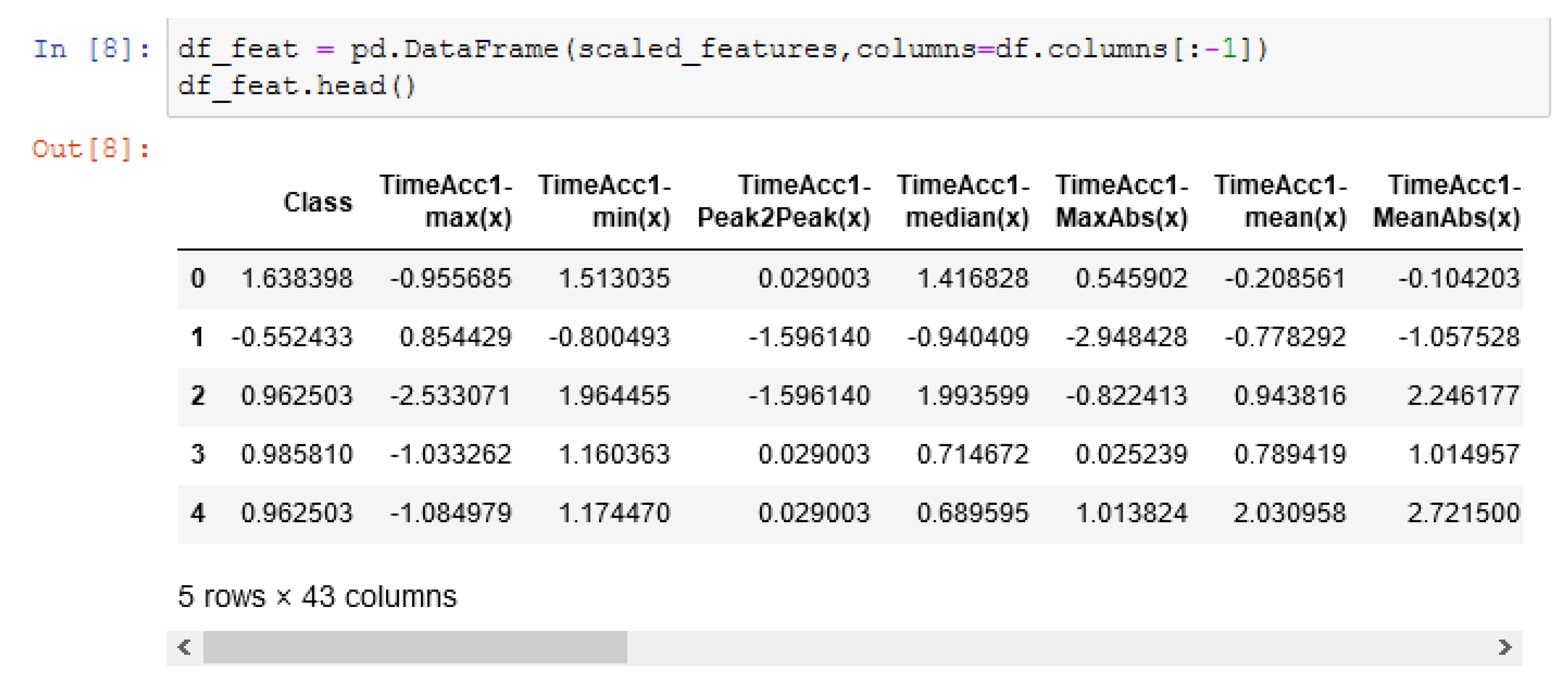
The aim of the research is a comparative analysis of selected algorithms for prediction and data analysis to determine the time and degree of tool usage in order to react early enough and avoid unwanted incidents affecting production optimization. The methods described in Section 2, i.e., K-nearest neighbors method, decision tree and linear regression, were used for data analysis and prediction. Apart from the selection of efficient classification methods, which can be used in real-time intelligent milling diagnostic systems, an important aspect is also the optimization of the time and quality of computation. This spectrum is strongly influenced by the parameters of these data mining algorithms, in particular, the learning process rate and the influence of the learning and testing set size value, which is also evaluated in this paper. Jupyter Notebook free software using Python programming language (Python Software Foundation, Wilmington, Delaware, USA) was used to create the algorithms based on the described methods [35,36]. The Numpy, pandas, matplotlib.puplot libraries were used for analysis. The sample data loaded for analysis in Jupyter were in the form presented in Figure 1. The data from the created set can be visualized in a line graph (Figure 2).
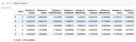
Figure 1.
Loading and presenting data in Jupyter software.

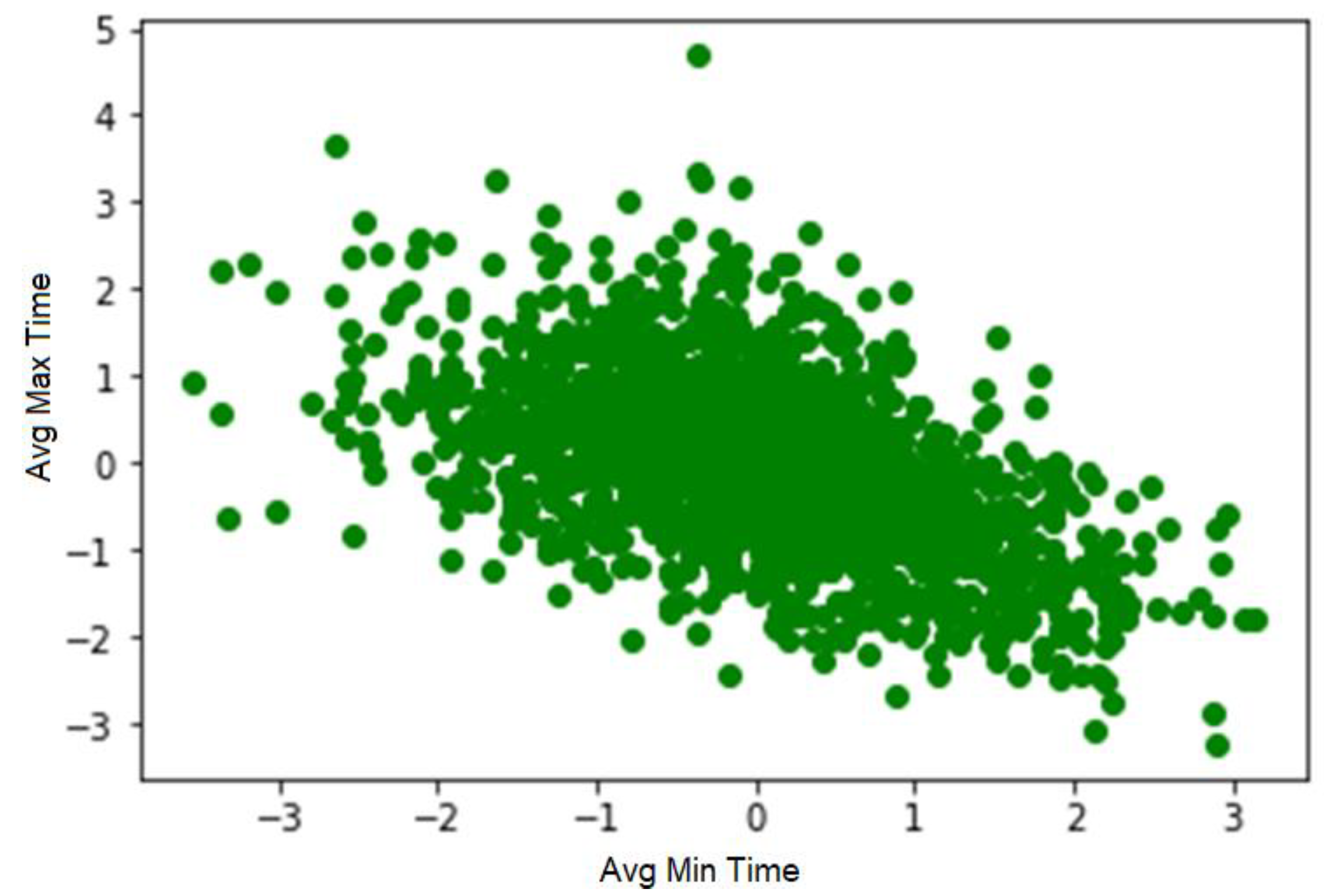
Figure 2.
Sample scatter plot visualization in Jupyter software.
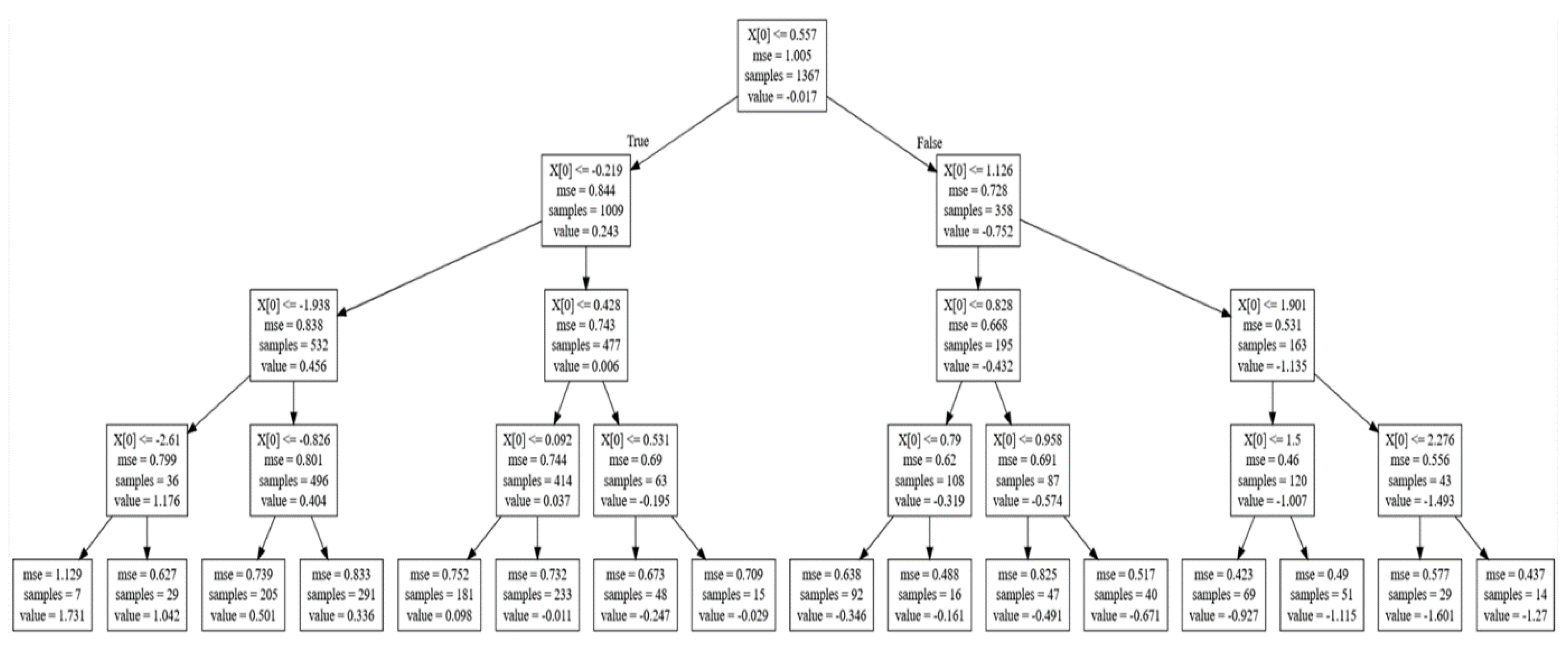
For the analyses based on the decision tree model, a feature function X was defined, which corresponds to the values found in the ‘TimeAcc1-min(x)’ column, and a goal function y, which is reflected in the ‘TimeAcc1-max(x)’ column. Next, a partitioning of the selected dataset into training and testing sets was performed, where the value of test_size = 0.2, which means that the testing set contains 20% of the total dataset and the training set contains 80% of the remaining data. Next, a regression decision tree model was built with parameters: max_depth = 4, min_samples_leaf 1. The generated decision tree in the form of a graph is illustrated in Figure 3.
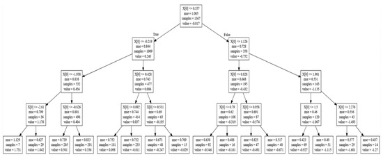
Figure 3.
The generated decision tree graph.
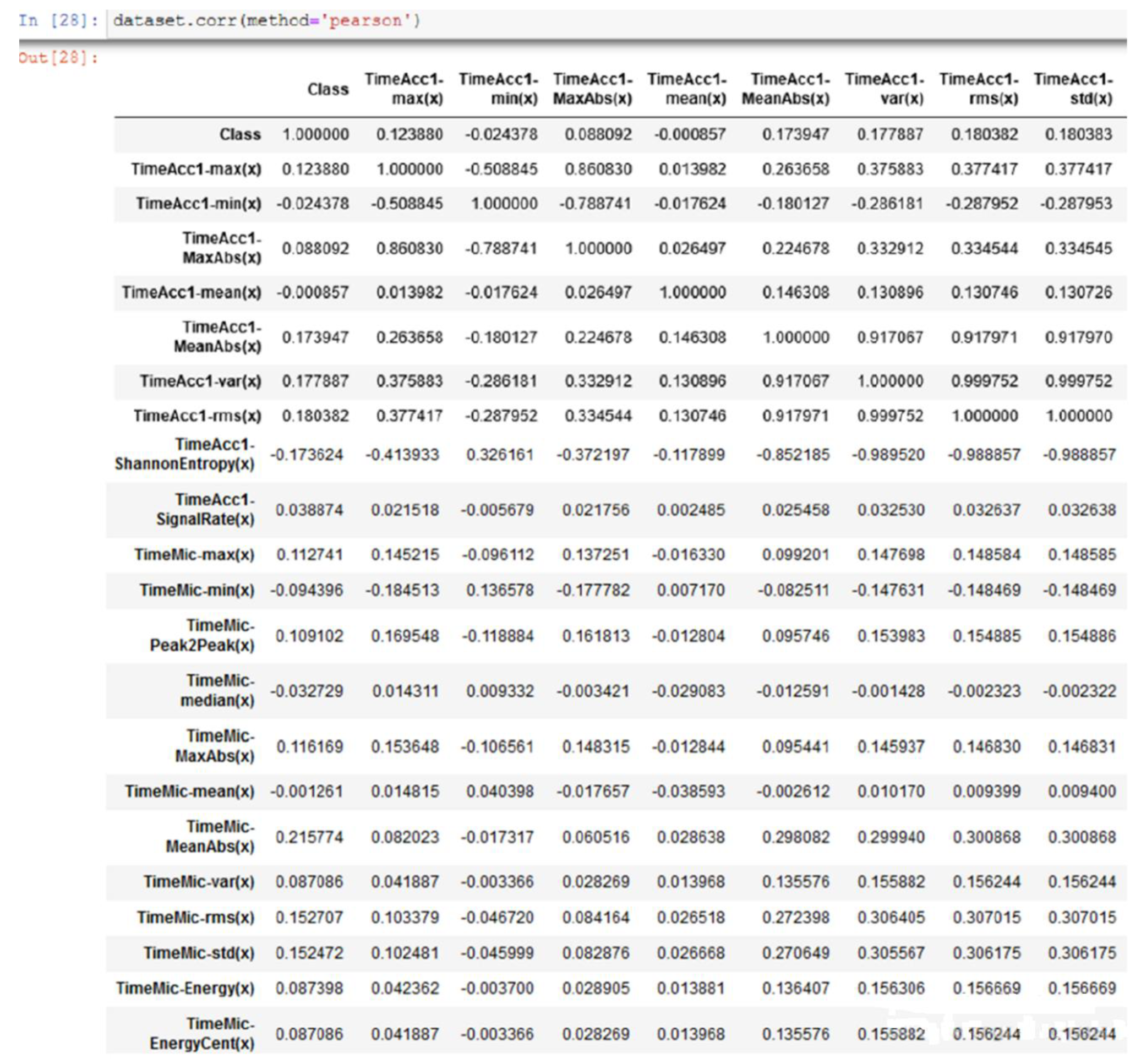
Jupyter Notebook application and Python programming language were also used to create a linear regression algorithm [35,36,37]. In the experiment, the Y value in the set of data values in the ‘TimeAcc1-median (x)’ column was subjected to prediction. In the next step, the correlation coefficient between the variables and the predictive variable was calculated. The correlation was performed using Pearson’s method, the results of which are illustrated in Figure 4.

Figure 4.
Correlation by Pearson’s method.
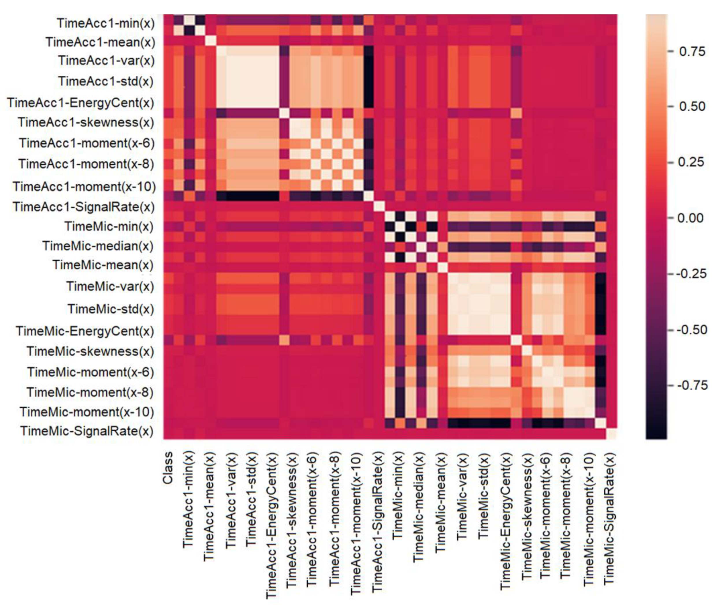
Moreover, a correlation table was generated for the above data—graphical visualization (see Figure 5).
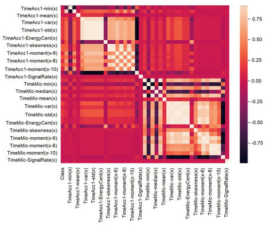
Figure 5.
Graphical visualization of the correlation table (Pearson’s method).
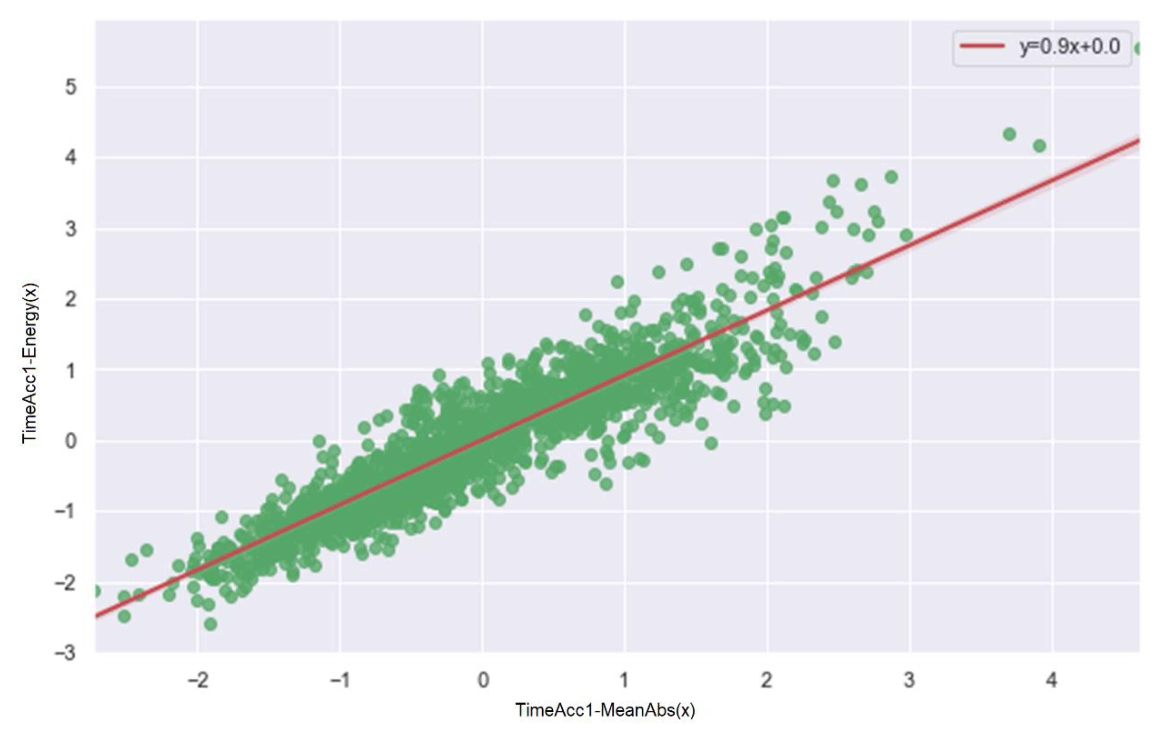
The statsmodel library was used to determine the variable that defines the value for the linear regression described [35,36,37]. For multiple linear regression, there are other techniques to narrow down the most important features or variables using what is called stepwise regression. Among these methods are techniques such as forward selection and backward elimination. A visualization of the linear regression determined on the analyzed set of data is shown in Figure 6. This graph was determined by using the libraries seaborn.regplot and scipy.stats.

Figure 6.
Linear regression graph.
In order to evaluate the obtained results and compare the correctness of linear regression data for ‘TimeACC1-mean(x)’ and ‘TimeAcc’ variables, Spearman’s monotonic correlation, Pearson’s linear correlation and Kendall’s monotonic correlation were used [35,36,37]. The obtained measurement results are presented in a summary Table 2.
Table 2.
Summary of results.
The computational speed analysis for each correlation was as follows:
- Spearman’s method = 25.2 ms ± 2.91 ms per loop (mean ± std dev of 7 runs, 10 loops each);
- Pearson’s method = 13.4 ms ± 2.93 ms per loop (mean ± std dev of 7 run, 10 loops each);
- Kendall’s method = 556 ms ± 51.9 ms per loop (mean ± std dev of 7 run, 1 loop each).
From the observed results, the best time was obtained by Pearson’s method, which was used in calculating the correlation for the linear regression algorithm.
The next step in the running of the K-nearest neighbors algorithm was to standardize the feature by removing the mean and scaling it to unit variance. This was done by centering and calibrating each feature using previously performed statistical calculations on samples in the learning sets. The results of this step are illustrated in Figure 7.

Figure 7.
Results of the standardization step.
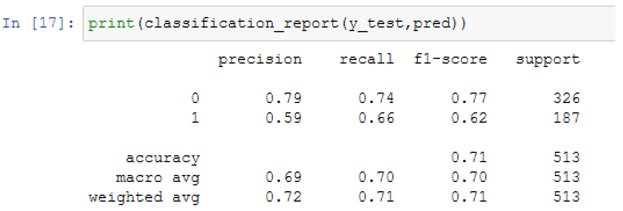
Partitioning of the selected dataset into training and testing sets was then performed. The analyses were performed for different ranges, which will be shown in detail in the next section. To illustrate the analysis process in detail, for the example, the value of test_size = 0.30 was determined, which means that the testing set contained 30% of the entire dataset and the training set contained 70% of the remaining data. In the next step, using the KNeighborsClassifier, the K-nearest neighbors classification was realized (and a text report was generated presenting all the classification metrics (see Figure 8). The metrics in the obtained report are described by columns:

Figure 8.
K-nearest neighbors classification results.
- Precision—defines the correctness of the classified elements;
- Recall—the number of classes in the given set;
- F1-score—the mean, harmonic between precision and sensitivity;
- Support—the number of occurrences of the class in the specified dataset.
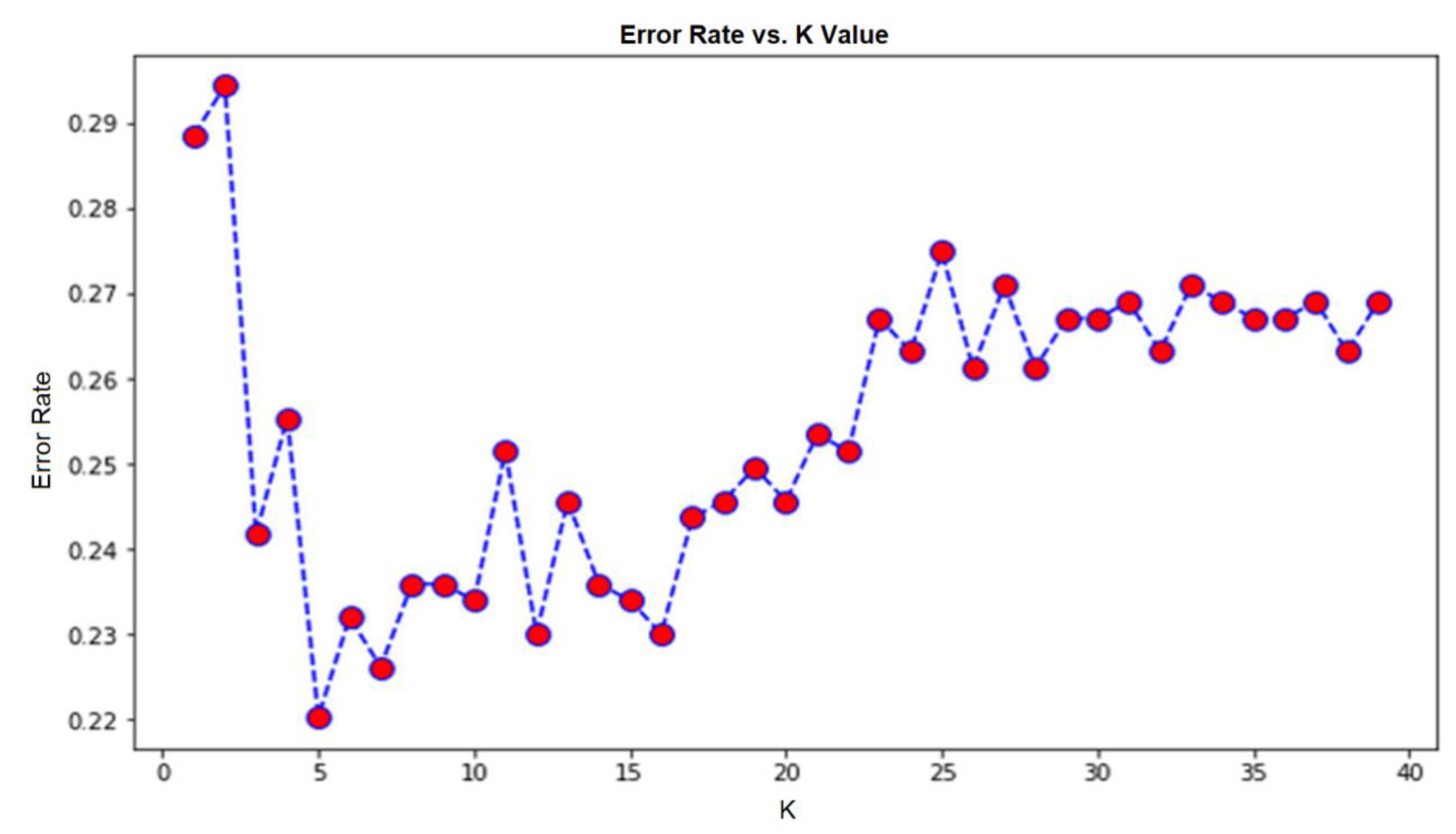
The error rate, including the value of K (1–40), is shown in Figure 9. The analysis of the obtained results shows that the minimum value of the error was 0.22.
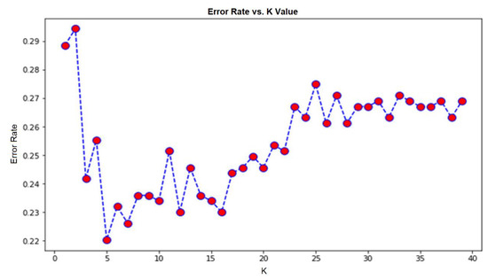
Figure 9.
The error rate graph.
In order to validate the measurements of the K-nearest neighbor method, an analysis was performed for different values of K, the results of which are shown in the table below (Table 3). The analysis was performed for K = 1, 200 and 800. The table lists the parameters that changed.
Table 3.
Results analysis for different K values.
Detailed analysis of the data shows that the accuracy (precision) decreased as the value of K of the group mean increased, while the percentage of the number of classes in a given set (recall) increased. For standard deviation, accuracy increased as the value of the number of classes in the collection decreased. It was also found that the harmonic mean for the mean group increased with the increase of the parameter K, while a significant decrease of these values for the standard deviation of the group was also observed. The number of occurrences of a given class in a given group had similar values. The numerical values of precision (accuracy), as well as weighted mean, were subject to change. Their values decreased with the increasing number of K.
5. Analysis of Models According to the Partition of the Test and Learning Set
The results obtained allow us to conclude that decision trees handle nonlinearity well in contrast to linear regression, which solves only linear equations. Having a large number of objects with fewer datasets (small amount of noise), one can find that linear regression is superior to decision trees in this aspect. In general cases, decision trees have better average (avg) accuracy, and independent qualitative variables will outperform linear regression. Comparing linear regression and K-nearest neighbors models, linear regression is a parametric model, unlike K-NN and decision trees, which are non-parametric. The big disadvantage of K-NN is its slow real-time performance, as the work of the algorithm consists of “tracking” all the learning data and finding the best neighboring node. The linear regression itself is characterized by the ease of extracting output from the tuned coefficients.
Figure 10, Figure 11, Figure 12, Figure 13, Figure 14, Figure 15, Figure 16, Figure 17, Figure 18 and Figure 19 present a summary of the results for testing and training values for each percentage.

Figure 10.
Summary of results for a testing dataset equal to 10% and training dataset of 90%.

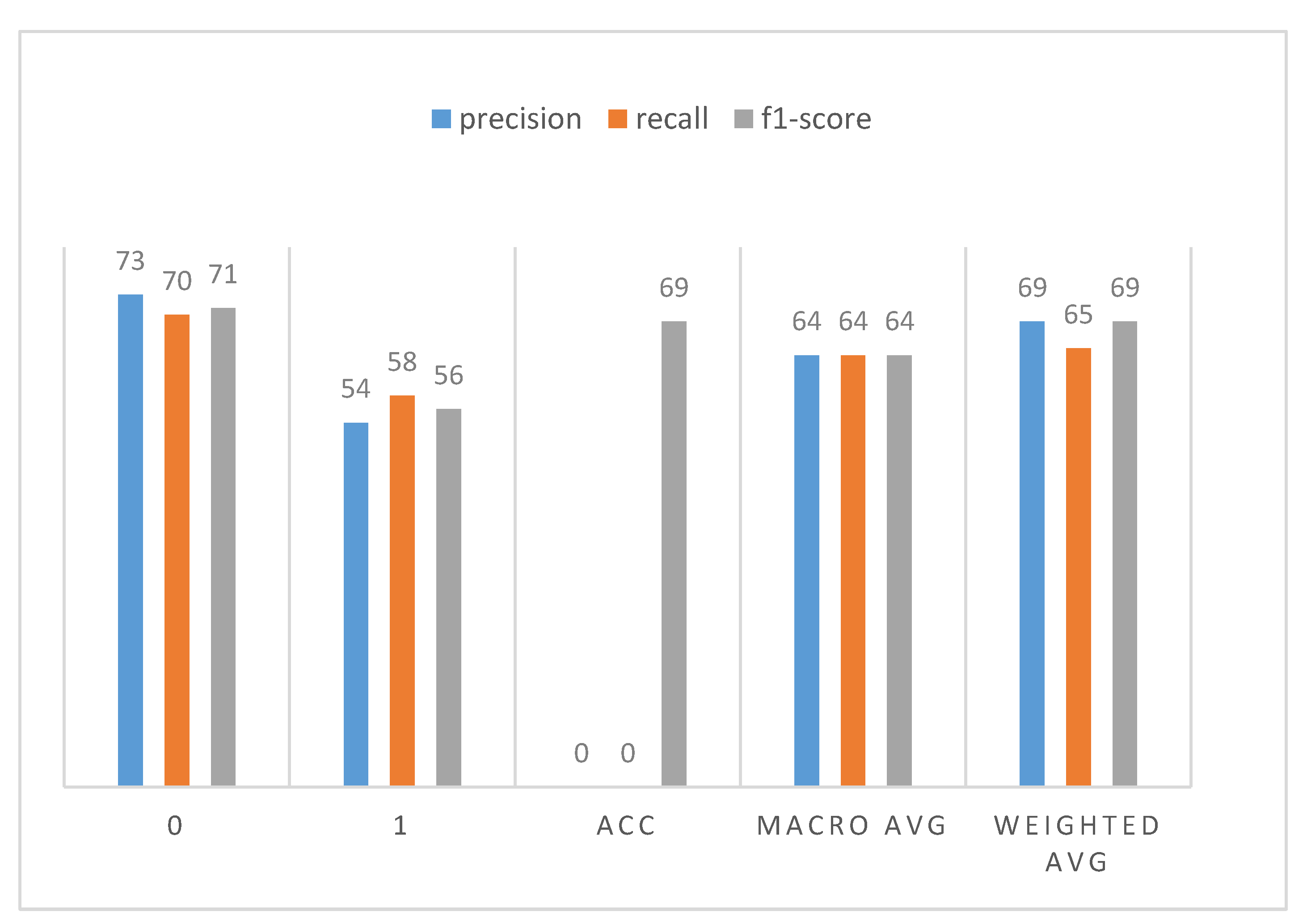
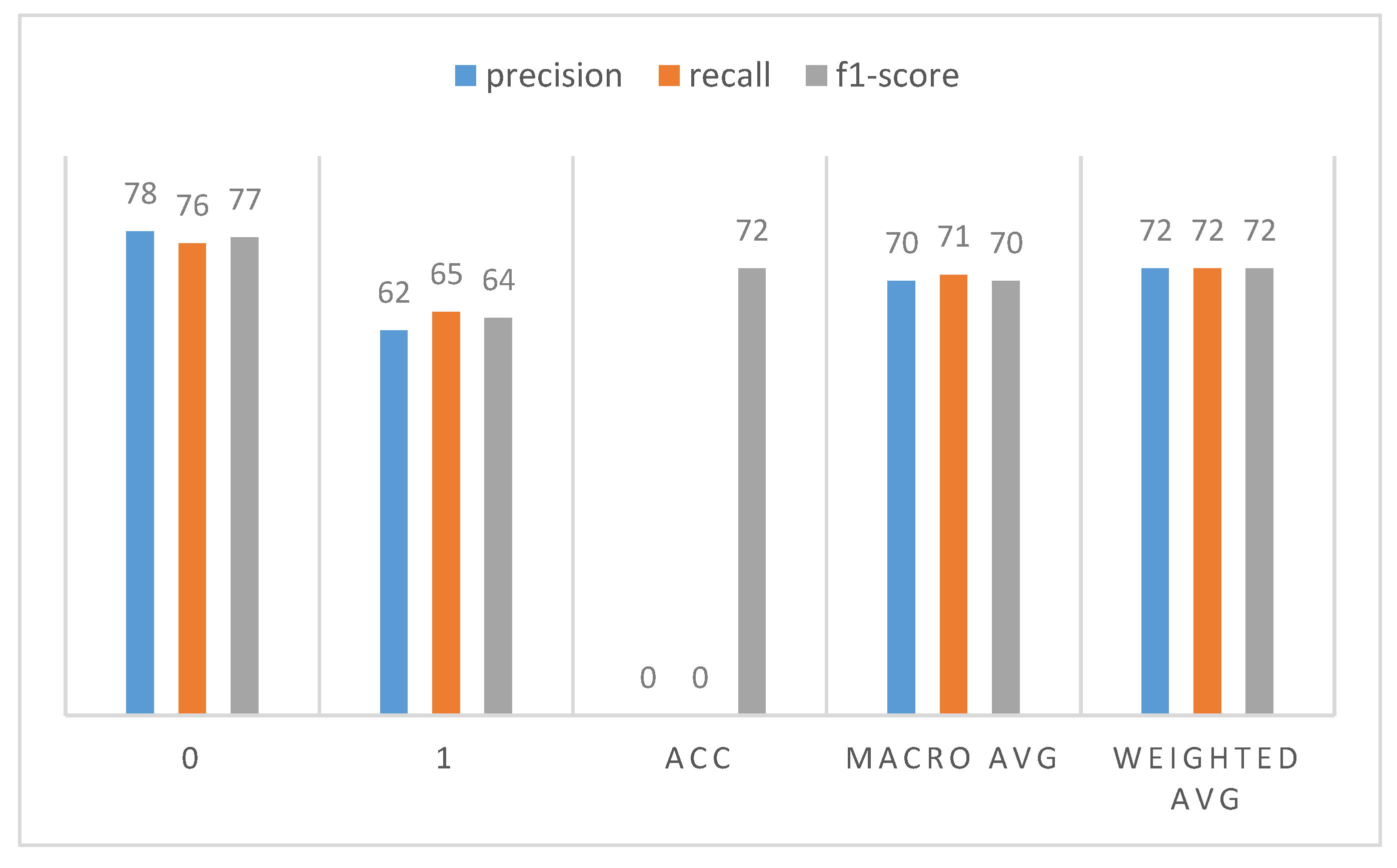
Figure 11.
Summary of results for a testing dataset equal to 20% and training dataset of 80%.

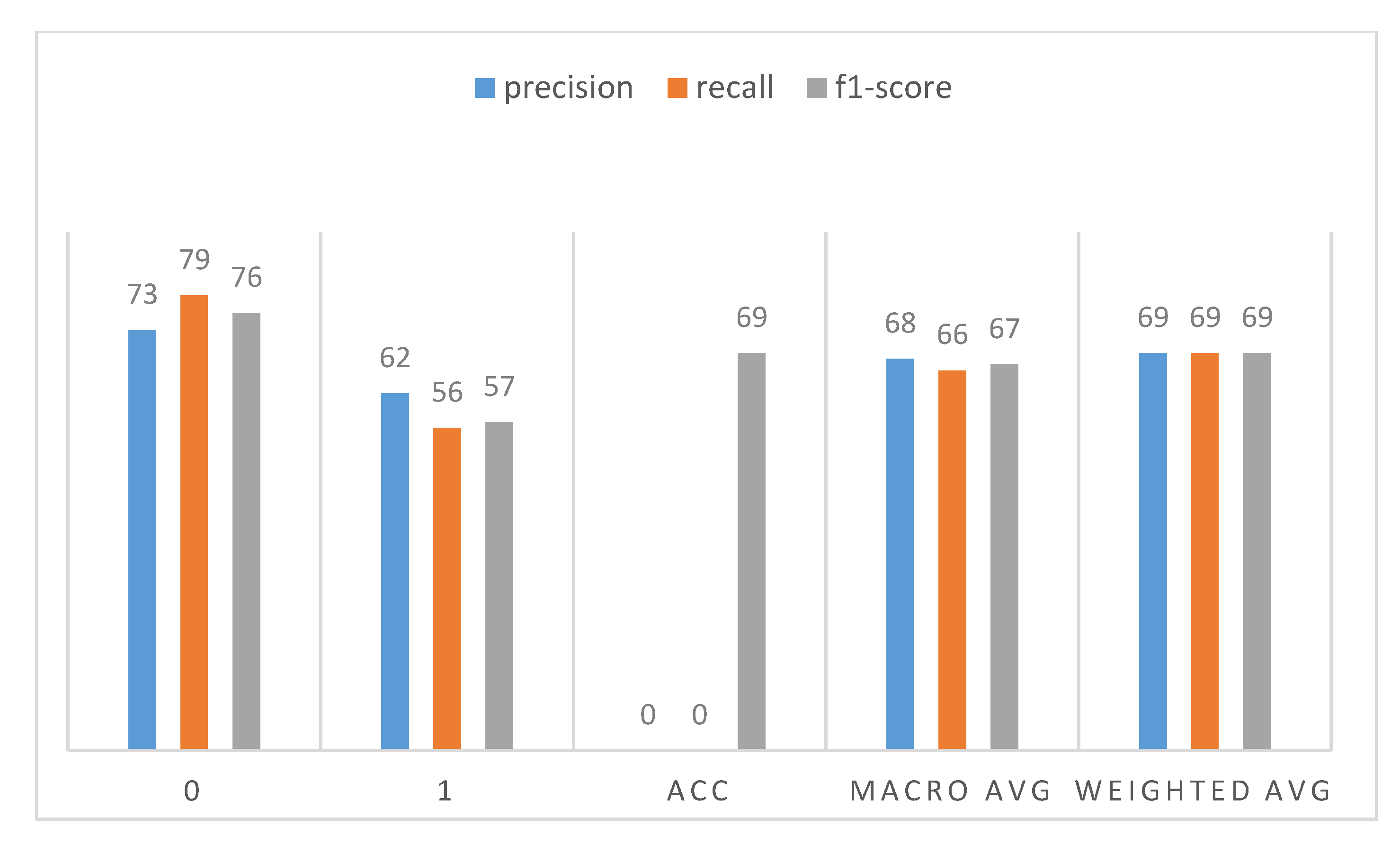
Figure 12.
Summary of results for a testing dataset equal to 30% and training dataset of 70%.

Figure 13.
Summary of results for a testing dataset equal to 40% and training dataset of 60%.

Figure 14.
Summary of results for a testing dataset equal to 50% and training dataset of 50%.

Figure 15.
Summary of results for a testing dataset equal to 60% and training dataset of 40%.

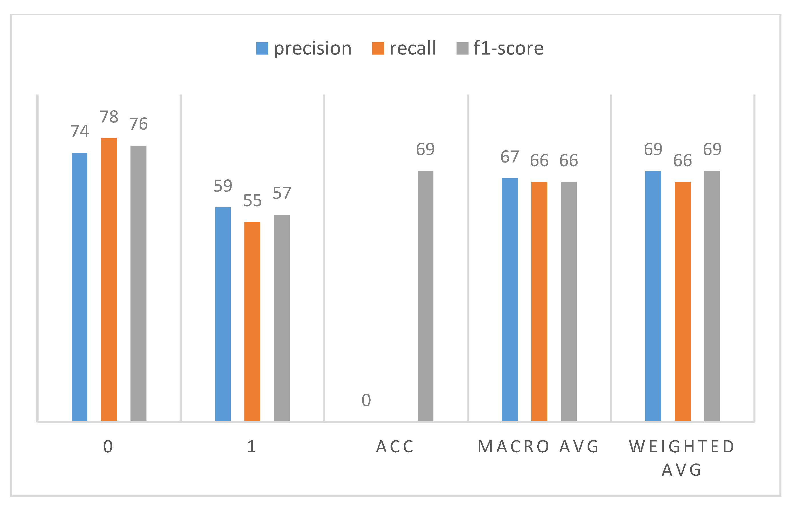
Figure 16.
Summary of results for a testing dataset equal to 70% and training dataset of 30%.

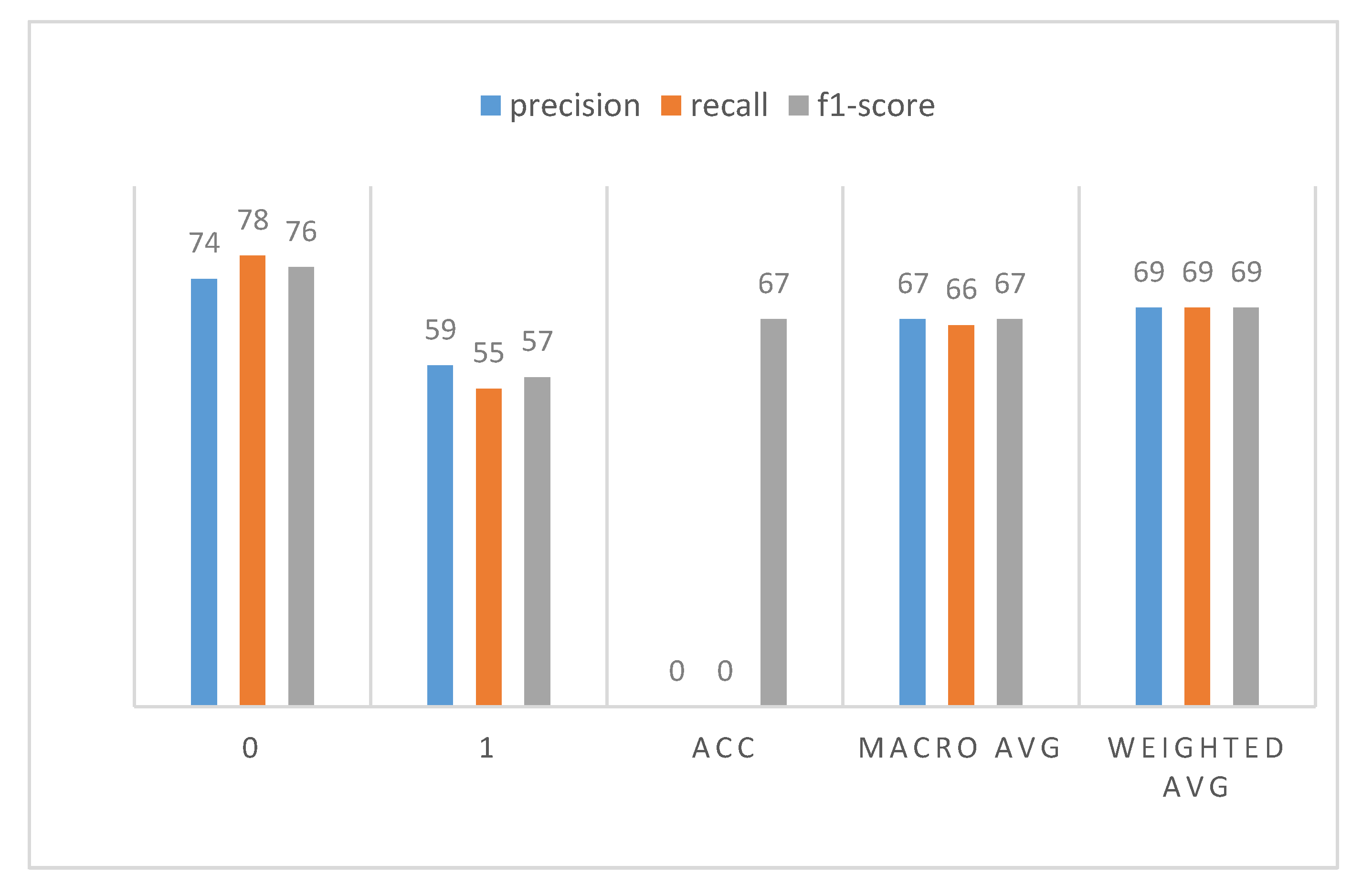
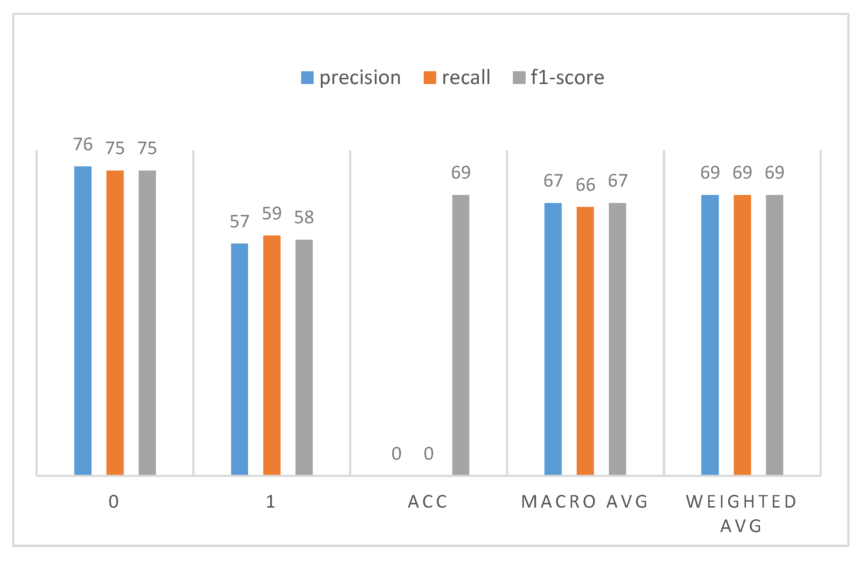
Figure 17.
Summary of results for a testing dataset equal to 80% and training dataset of 20%.

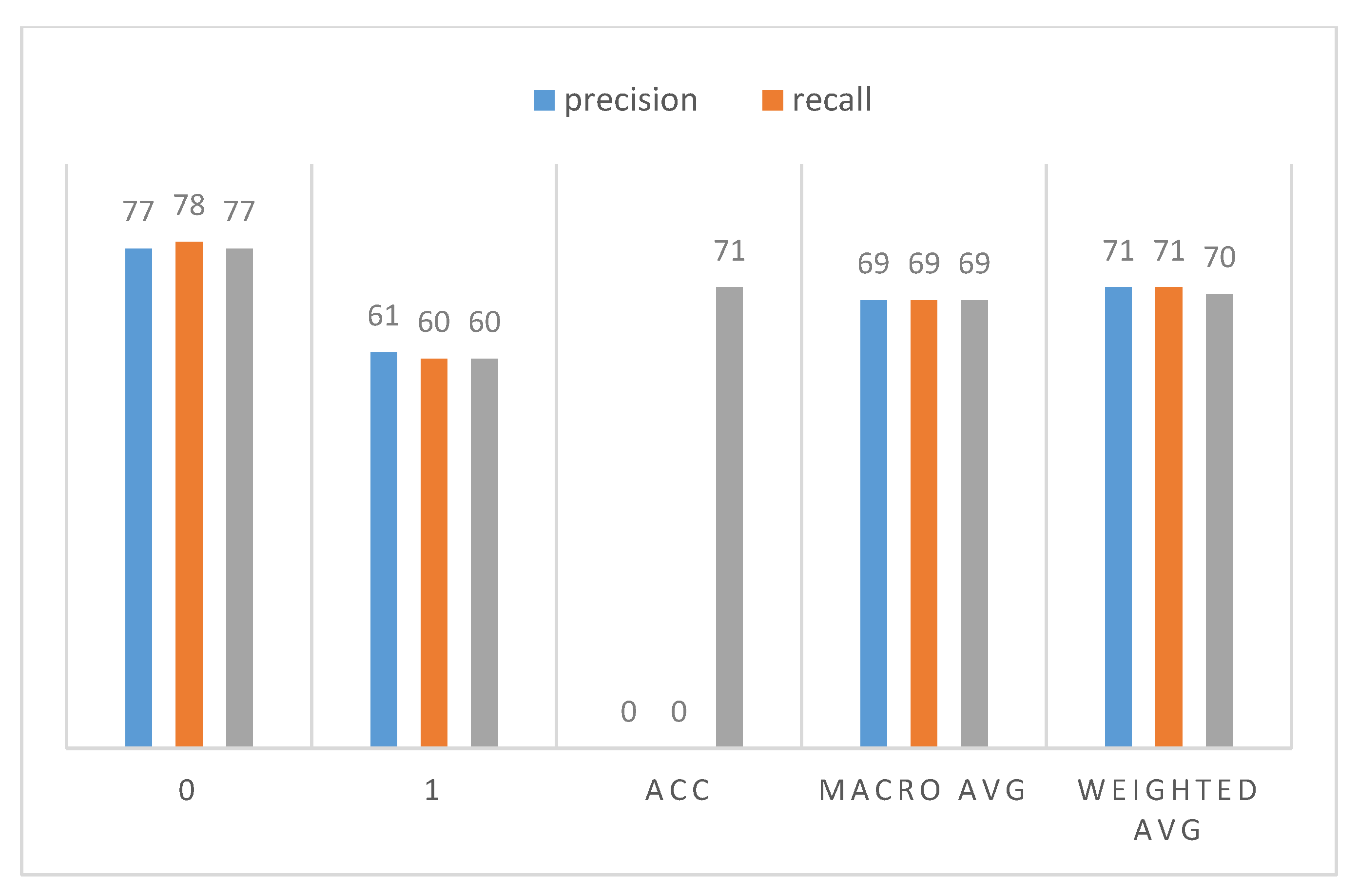
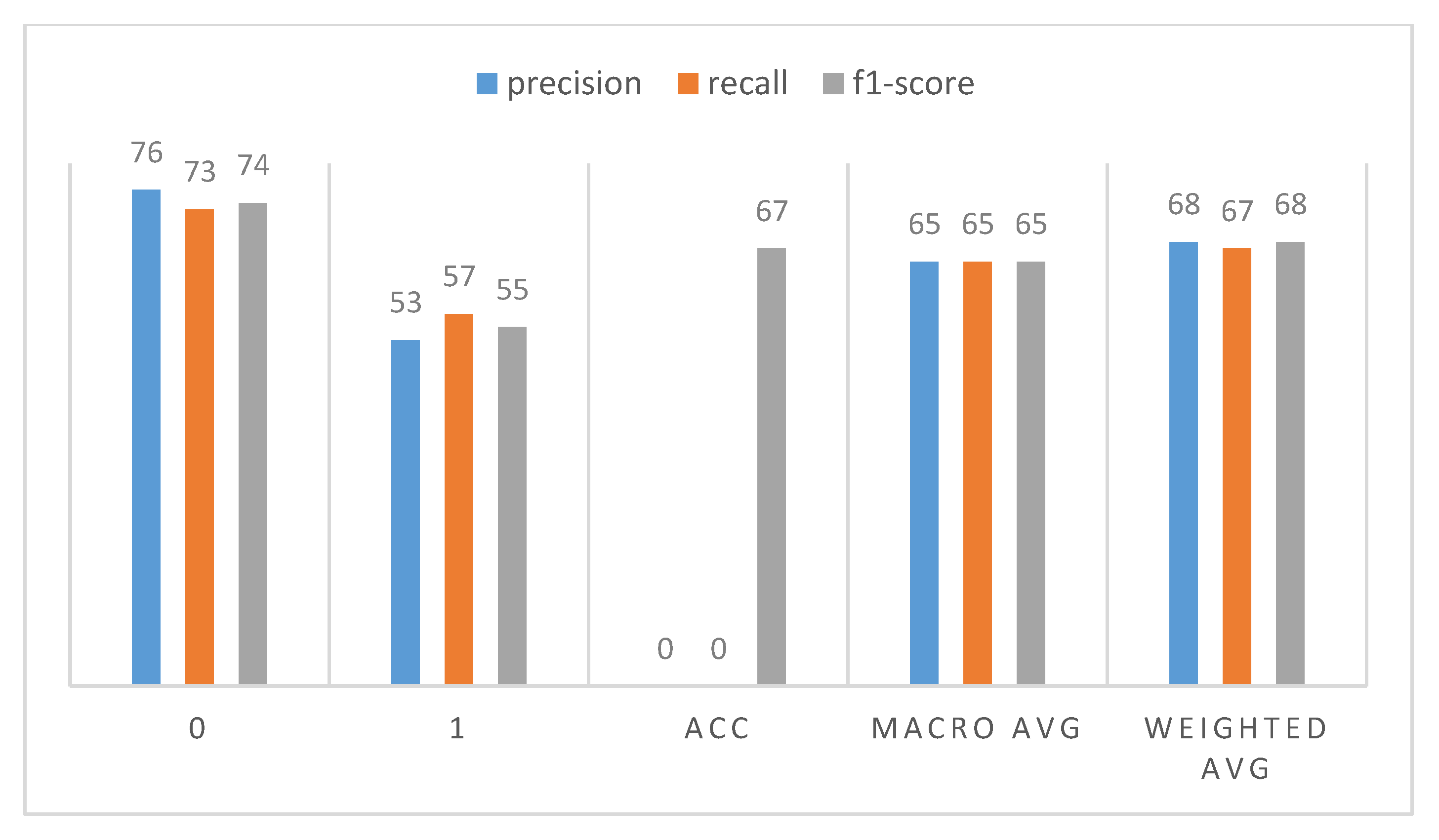
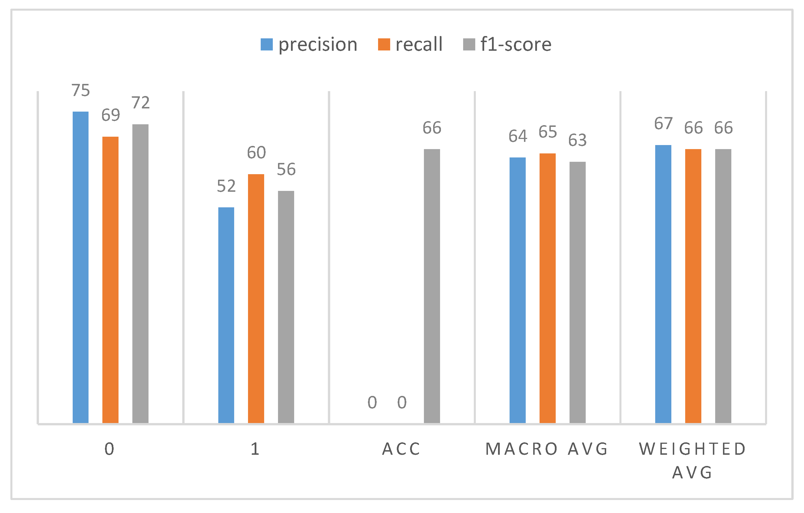
Figure 18.
Summary of results for a testing dataset equal to 90% and training dataset of 10%.

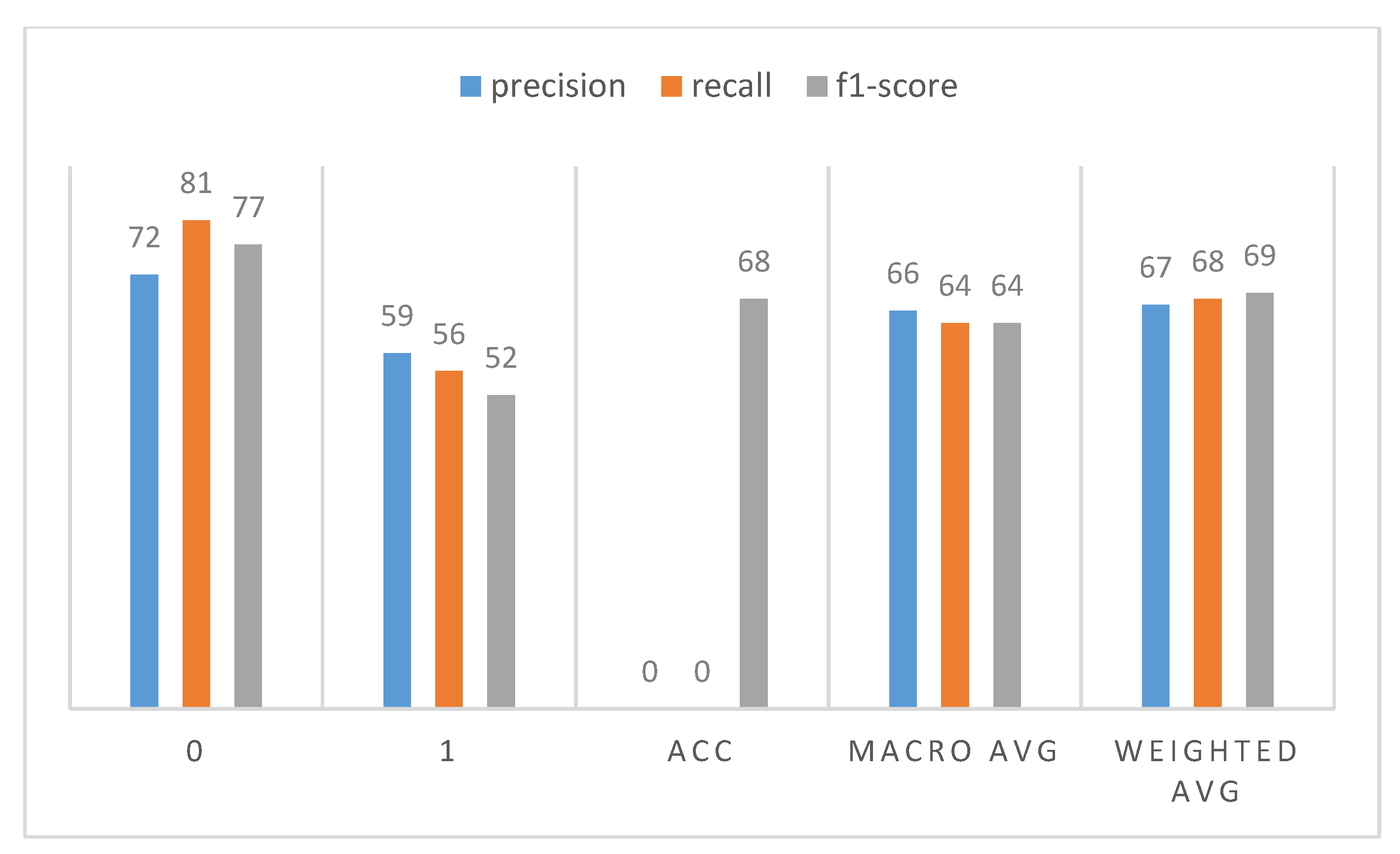
Figure 19.
Summary of results for a testing dataset equal to 99% and training dataset of 1%.
In Figure 10, it can be seen that the range for class (0) was the highest for the metrics used, in contrast to the range for class (1). The value of the macro mean remained constant, while the values of the weighted mean varied slightly for each parameter.
For the testing dataset size equal to 20% and 80% for training dataset values (Figure 11), the weighted average values leveled off, while the precision value for the lower limit increased from 54% to 62%.
For the testing dataset size of 30% and training dataset size of 70% (Figure 12), one parameter—precision for the lower limit—decreased. For the other values, there was no significant decrease or increase.
A greater difference between the specified parameters can be seen for the values of the test dataset equal to 40% and training dataset size 60% (Figure 13). As the percentage of testing data increased and the percentage of training data decreased, it was noted that the values for all parameters were at a consistently high level.
Figure 14 illustrates the best combination of results that were seen for the 50% testing and training datasets. No significant jumps for individual parameters were observed here.
With an increase in the percentage for the test dataset size to 60%, a significant decrease was noticed in Figure 15 for class 1, in contrast to the graph of Figure 14. The other parameters remained constant.
The results presented in Figure 16 are not significantly different from the graph presented in Figure 15. Changing the size of the training (30%) and testing (70%) dataset did not affect the values of the individual parameters to a large extent.
Figure 17 shows a summary of the results for a test dataset size of 80% and a training dataset size of 20%. It can be clearly seen that the percentage of the number of classes in a given set increased for class 0. For class 1, it decreased from 59% to 55%, which can also be seen in the individual graphs.
In Figure 18, an increase in the percentage of the number of classes in a given set for class 1 becomes apparent. The values for the macro average and weighted average decreased with a test dataset size of 90% and a training dataset size of 10%.
Figure 19 shows the largest decrease in all three parameters for class 1. With a testing dataset equal to 99% and the training dataset of 1%, the percentage of the number of classes in a given set for class 0 was the highest among all sets of results.
Interpreting the graphs above, it can be concluded that the range of precision for class (0) varied from 72% to 78%, thus concluding that the data had very similar values because they came from a very precise device. Class 1 was characterized by a lower limit, the so-called worst result, where the tolerance was already in the range from 52% to 62%. The weighted average was virtually identical, which may suggest a slight variation in the variables. The best set of parameters for the test and training data was the 50/50% range, as it gave the best upper range, precision range 78% and lower range 61%. The mean values were at the high level of 70–72%. The worst range for the experiments was 10% testing data and 90% training data. Despite the high precision of the upper range 75%, the lower range was 52%, which was not the worst value. These average values were significantly different, which may mean that too little testing data can affect the good interpretation and correctness of the algorithm performed. When interpreting the number of classes in the set values for each dataset percentage size, the results obtained were strongly similar. Analyzing the comparative data of the f1-score value for each dataset percentage size also showed that the 50/50% testing and training datasets gave the best results.
6. Conclusions
A comparative analysis of selected algorithms for prediction and data analysis is presented in this paper. The research is based on K-nearest neighbor, decision tree and linear regression algorithms on a set of data taken from a CNC milling machine.
The extraction of statistical parameters in the time and frequency domain from the cutting force signals allowed the determination of an effective and efficient classifier with minimum response time, which is the basis for the operation of the TCM process. The conducted analyses showed that there is a need for a detailed study of the nature of the signal and its relationship to the tool condition, especially in the case of an intermittent cutting process. The signal features such as statistical features, histogram features, empirical modal decomposition (EMD) features, discrete wavelet transform (DWT) features and artificial intelligence techniques, decision tree, fuzzy neural network, Bayesian network, Markov model are applied in the TCM system.
The satisfactory correlation of various signals such as cutting force, vibration, spindle current and sound signals is the success of the research. The analysis of vibration during milling will allow the prediction of tool damage, for example, using cutting force signals. RQA (quantitative recurrence analysis) parameters, such as entropy, laminarity percentage, capture time and repeatability percentage, are useful features for detecting wear on the cutting surface of a tool. The control system plays an equally important role in the cutting tool condition monitoring system. Research confirms that a system consisting of expert rule-based modules for selecting cutting parameters such as tool life, material removal rate, workpiece surface roughness and stability in the milling process is the basis for trouble-free machine operation.
Of the algorithms discussed, the decision tree provided the simplest and quickest way to explain the results. Most understand the hierarchical nature of the tree, and the clarity of the diagram can improve the quality of the results obtained. The decision tree algorithm has easy-to-use functions for identifying the most important dimensions, handling missing values and dealing with outliers. Although over-fitting is the main problem of this algorithm, it can be avoided by using the method of boosted trees or random forests. The fewer the number of branches of a given tree, the more accurate the results. Unlike the K-NN algorithm, decision trees can work directly on data tables without any preliminary design work. The advantage of this technique is that the classifiers are selected from the data table without the need to know them, which facilitates rapid implementation.
The advantage of the K-nearest neighbors algorithm is, as in the case of the tree, simplicity in use and implementation. K-NN is characterized by high robustness to isolated values by evaluating their nearest neighbors. The big problem with this algorithm is the memory requirements and the need to input K values. The larger the database, the longer the classification time. Linear regression is the most applicable method in everyday life. It is used in scientific fields by all researchers. The calculation can be done manually as well as with the help of various statistical applications.
Detailed analyses showed that accuracy (precision) decreased as the value of K of the group mean increased, while the percentage of the number of classes in a given set (recall) increased. For standard deviation, accuracy increased as the value of the number of classes in the collection decreased. It was also found that the harmonic mean for the mean group increased with an increase in the parameter K, while a significant decrease in these values was also observed for the standard deviation of the group. The numerical value of precision (accuracy) decreased with increasing K.
As the conducted research shows, the appropriate choice of algorithms, especially the proportion of dataset partitioning into a learning set and a test set, are crucial in advanced data analysis and mining. In further work, it is expected to use the obtained results for testing and detection of anomalies in the operation of CNC machines, which will allow for detecting in advance the impending damage to the tool on the basis of the monitored parameters to avoid costly downtime. Thus, the use of learning algorithms for data mining and prediction can significantly increase the efficiency of modern factories in the context of Industry 4.0.
Author Contributions
Methodology, P.D., S.B. and M.M.; software: formal analysis and investigation, P.D. and M.M.; conceptualization P.D. and M.M.; resources: P.D., S.B. and M.M.; writing—original draft preparation, P.D. and M.M; writing—review and editing, P.D. and M.M; visualization: P.D., S.B. and M.M.; supervision, P.D. and M.M; project administration, P.D. and M.M. All authors have read and agreed to the published version of the manuscript.
Funding
This research paper was developed under the project financed by the Minister of Education and Science of the Republic of Poland within the “Regional Initiative of Excellence” program for years 2019–2022. Project number 027/RID/2018/19, amount granted 11 999 900 PLN.
Institutional Review Board Statement
Not applicable.
Informed Consent Statement
Not applicable.
Data Availability Statement
Not applicable.
Conflicts of Interest
The authors declare no conflict of interest.
References
- Sedgewick, R.; Wayne, K. Algorytmy, Wydanie IV; Helion: Gliwice, Poland, 2012; 952p, ISBN 978-83-246-3536-8. [Google Scholar]
- Dymora, P.; Paszkiewicz, A. Performance Analysis of Selected Programming Languages in the Context of Supporting Decision-Making Processes for Industry 4.0. Appl. Sci. 2020, 10, 8521. [Google Scholar] [CrossRef]
- Ramadan, M.; Shuqqo, H.; Qtaishat, L.; Asmar, H.; Salah, B. Sustainable Competitive Advantage Driven by Big Data Analytics and Innovation. Appl. Sci. 2020, 10, 6784. [Google Scholar] [CrossRef]
- Mallak, A.; Fathi, M. A Hybrid Approach: Dynamic Diagnostic Rules for Sensor Systems in Industry 4.0 Generated by Online Hyperparameter Tuned Random Forest. Science 2020, 2, 75. [Google Scholar] [CrossRef]
- Serradilla, O.; Zugasti, E.; de Okariz, J.R.; Rodriguez, J.; Zurutuza, U. Adaptable and Explainable Predictive Maintenance: Semi-Supervised Deep Learning for Anomaly Detection and Diagnosis in Press Machine Data. Appl. Sci. 2021, 11, 7376. [Google Scholar] [CrossRef]
- Dymora, P.; Mazurek, M. An Innovative Approach to Anomaly Detection in Communication Networks Using Multifractal Analysis. Appl. Sci. 2020, 10, 3277. [Google Scholar] [CrossRef]
- Dymora, P.; Mazurek, M. Influence of Model and Traffic Pattern on Determining the Self-Similarity in IP Networks. Appl. Sci. 2020, 11, 190. [Google Scholar] [CrossRef]
- Martin, R.; Christian, L.; Roland, Z.; Andreas, R.; Andrea, H.; Gunther, R. Smart Grid for Industry Using Multi-Agent Reinforcement Learning. Appl. Sci. 2020, 10, 6900. [Google Scholar] [CrossRef]
- Byrne, G.; Dornfeld, D.; Inasaki, I.; Ketteler, G.; König, W.; Teti, R. Tool Condition Monitoring (TCM) The Status of Research and Industrial Application. CIRP Ann. 1995, 44, 541–567. [Google Scholar] [CrossRef]
- Narayanan, A.; Kanyuck, A.; Gupta, S.K.; Rachuri, S. Machine Condition Detection for Milling Operations Using Low Cost Ambient Sensors. In Proceedings of the ASME 11th International Manufacturing Science and Engineering Conference, Blacksburg, VA, USA, 27 June–1 July 2016. [Google Scholar]
- Ryabov, O.; Mori, K.; Kasashima, N.; Uehara, K. An In-Process Direct Monitoring Method for Milling Tool Failures Using a Laser Sensor. CIRP Ann. 1996, 45, 97–100. [Google Scholar] [CrossRef]
- LoCasto, S.; LoValvo, E.; Micari, F.; Ruisi, V.F. Tool wear measured by computer vision. C.S.M.E. Mech. Eng. Forum 1990, 3, 59–63. [Google Scholar]
- Park, J.-J.; Ulsoy, A.G. On-Line Flank Wear Estimation Using an Adaptive Observer and Computer Vision, Part 2: Experiment. J. Eng. Ind. 1993, 115, 37–43. [Google Scholar] [CrossRef]
- Wang, G.; Guo, Z.; Yang, Y. Force sensor based online tool wear monitoring using distributed Gaussian ARTMAP network. Sens. Actuators A Phys. 2013, 192, 111–118. [Google Scholar] [CrossRef]
- Elangovan, M.; Ramachandran, K.; Sugumaran, V. Studies on Bayes classifier for condition monitoring of single point carbide tipped tool based on statistical and histogram features. Expert Syst. Appl. 2010, 37, 2059–2065. [Google Scholar] [CrossRef]
- Madhusudana, C.; Kumar, H.; Narendranath, S. Condition monitoring of face milling tool using K-star algorithm and histogram features of vibration signal. Eng. Sci. Technol. Int. J. 2016, 19, 1543–1551. [Google Scholar] [CrossRef] [Green Version]
- Kusy, M.; Kluska, J.; Zajdel, R.; Zabiński, T. Fusion of Feature Selection Methods for Improving Model Accuracy in the Milling Process Data Classification Problem; IEEE: Piscatway, NJ, USA, 2020. [Google Scholar]
- Goebel, K.; Yan, W. Feature Selection for Tool Wear Diagnosis Using Soft Computing Techniques. ASME Int. Mech. Eng. Congr. Exhib. 2000, 157–163. [Google Scholar] [CrossRef]
- Dymora, P.; Mazurek, M. Comparison of Selected Algorithms of Traffic Modelling and Prediction in Smart City—Rzeszów. In Theory and Engineering of Dependable Computer Systems and Networks. DepCoS-RELCOMEX 2021. Advances in Intelligent Systems and Computing; Zamojski, W., Mazurkiewicz, J., Sugier, J., Walkowiak, T., Kacprzyk, J., Eds.; Springer: Cham, Switzerland, 2021; Volume 1389. [Google Scholar] [CrossRef]
- Gangadhar, N.; Kumar, H.; Narendranath, S. Condition monitoring of single point cutting tool through vibration signals using decision tree algorithm. J. Vib. Anal. 2015, 3, 34–43. [Google Scholar]
- Painuli, S.; Elangovan, M.; Sugumaran, V. Tool condition monitoring using K-star algorithm. Expert Syst. Appl. 2014, 41, 2638–2643. [Google Scholar] [CrossRef]
- Sakthivel, N.R.; Nair, B.B.; Elangovan, M.; Sugumaran, V.; Saravanmurugan, S. Comparison of dimensionality reduction techniques for the fault diagnosis of monoblock centrifugal pump using vibration signals. Eng. Sci. Technol. Int. J. 2014, 17, 30–38. [Google Scholar]
- Sugumaran, V.; Ramachandran, K. Fault diagnosis of roller bearing using fuzzy classifier and histogram features with focus on automatic rule learning. Expert Syst. Appl. 2011, 38, 4901–4907. [Google Scholar] [CrossRef]
- Sugumaran, V.; Muralidharan, V.; Ramachandran, K. Feature selection using Decision Tree and classification through Proximal Support Vector Machine for fault diagnostics of roller bearing. Mech. Syst. Signal Process. 2007, 21, 930–942. [Google Scholar] [CrossRef]
- Alonso, F.J.; Salgado, D.R. Analysis of the structure of vibration signals for tool wear detection. Mech. Syst. Signal Proces. 2008, 22, 735–748. [Google Scholar] [CrossRef]
- Mirończuk, M. Przegląd i klasyfikacja zastosowań, metod oraz technik eksploracji danych. Politech. Białostocka Studia Mater. Inform. Stosow. 2010, 2, 35–46. [Google Scholar]
- Wachla, D. Odkrywanie wiedzy w bazach danych jako proces identyfikacji modeli diagnostycznych. Diagnostics 2004, 30, 175–178. [Google Scholar]
- Bahri, A.; Sugumaran, V.; Devasenapati, S.B. Misfire detection in IC engine using Kstar algorithm. arXiv 2013, arXiv:1310.3717. [Google Scholar]
- Breiman, L.; Freidman, J.H.; Olshen, R.A.; Stone, C.J. Classification and Regression Trees; CRC Press: Boca Raton, FL, USA, 1984. [Google Scholar]
- Dymora, P.; Mazurek, M.; Łannik, D. Analiza wpływu wybranych implementacji algorytmu drzewa decyzyjnego na wydajność systemu komputerowego. In Monografia pt. Social and Technical Aspects of Security; Oficyna Wydawnicza Politechniki Rzeszowskiej: Rzeszów, Poland, 2020; ISBN 978-83-7934-354-6. [Google Scholar]
- Brownlee, J. Master Machine Learning Algorithms. Discover How They Work and Implement Them from Scratch; Machine Learning Mastery: San Juan, Puerto Rico, 2016; p. 163. [Google Scholar]
- Brownlee, J. Simple Linear Regression Tutorial for Machine Learning. 2016. Available online: https://machinelearningmastery.com/simple-linear-regression-tutorial-for-machine-learning/ (accessed on 1 August 2021).
- Rubikowska, B.; Włodarczyk, M. Regresja Logistyczna Algorytm Estymacji Współczynników i Przykład Zastosowania w Pakiecie Statystycznym R; Uniwersytet Warszawski: Warsaw, Poland, 2012. [Google Scholar]
- Jupyter. Available online: https://jupyter.org/ (accessed on 1 August 2021).
- Galea, A. Applied Data Science with Python and Jupyter; Packt: Birmingham, UK, 2019. [Google Scholar]
- Ascher, D.; Lutz, M. Python. Wprowadzenie; Helion: Gliwice, Poland, 2020; 368p, ISBN 83-719-7596-1. [Google Scholar]
- Jianqiang, Z.; Xiaolin, G. Comparison Research on Text Pre-processing Methods on Twitter Sentiment Analysis. IEEE Access 2017, 5, 2870–2879. [Google Scholar] [CrossRef]

Publisher’s Note: MDPI stays neutral with regard to jurisdictional claims in published maps and institutional affiliations. |
© 2022 by the authors. Licensee MDPI, Basel, Switzerland. This article is an open access article distributed under the terms and conditions of the Creative Commons Attribution (CC BY) license (https://creativecommons.org/licenses/by/4.0/).