1. Introduction
In recent years, the decrease of CO
emissions from power generation has been the main concern to improve the environment [
1]. In common with the many ways to generate energy, grid-connected inverters are frequently found in this type of system to regulate the grid voltage or frequency. The grid-connected inverters are devices that can integrate the electrical grid to the renewable energy source for distributed generation (DG) systems [
2].
In [
3], a proportional resonant (PR) control approach is used through a dual-loop current to link the inverter to the electrical grid. The model is based on a grid with an LCL-filter connected between the grid and the inverter in discrete domain under a stationary frame; this presents the practicality and robustness of the proportional PR. The authors in [
4] propose a controller that through grid current feedback active damping can provide the desired bandwidth and robustness against the parameter variation. Another type of controller that can be considered uses a proportional and integral controller with the resonant part that can achieve zero steady-state error [
5]. These examples of controllers are part of countless types of controllers that can be divided into classic controllers, predictive controllers, repetitive controllers, robust controllers, and non-linear controllers. All of them can be single-input and single-output (SISO) and multiple-input-multiple-output (MIMO) [
6].
The model predictive control (MPC) is a class of controllers that predicts the behavior of specific variables of the system through the model and chooses the controller outputs minimizing the cost function [
7]. This type of controller is limited in the number of voltage vectors, which results in a variable switching frequency that interferes with the filters for grid-connected systems [
8]. The MPC can be implemented using a pulse width modulation (PWM) to solve the variation frequency problem that exists in the finite control set (FCS). The MPC technique has been proposed for induction motor drives [
9], doubly-fed induction generators [
10], or inverters.
Repetitive control (RC) [
11] is based on the internal model [
12] using a transfer function (TF), which is a mathematical representation of the system relating the output and the input in the frequency domain. Another way to represent the system is the state-space (SS) model using the input to output the state variables correlated to the first-order differential of the states (most commonly uses the current and voltage); in the cases of both TF or SS, it is using a periodic signal as a reference [
6]. The internal model can provide a zero-error tracking of the reference. For this, it is necessary to include a polynomial equation for the controller [
13]. Applications for robotic and power electronics can use this controller [
14,
15,
16].
A conventional MPC can be susceptible to parameter variation. To improve the robustness of an MPC, a compensated RC scheme is combined to the system as in [
17]. The idea of parameter variation can also be solved through robust control as in [
18], where the approach focuses on robust predictive control with space vector modulation (SVM).
In contrast, ref. [
19] features robust predictive control, but using discrete space vector modulation (DSVM), which provides a finite combination of the eight inverter voltage vectors. Still discussing robust control for grid connected systems in [
20], the authors analyze the robustness of the controller for possible grid-impedance variations, which justify the effort to study this subject. One of the application examples is in [
21,
22]. These articles demonstrated the use of robust controls in a doubly fed induction generator (DFIG), which can be found in wind energy systems. When a robust control is applied in this kind of system, the benefits can be the guarantee of a good performance from uncertain parameter values and disturbances that occur in practical situations. These disturbances may include an unbalanced and distorted voltage, which is the focus of [
23]. In addition to robust control, the authors use a phase locked loop (PLL) scheme to extract a filtered wave form to use as a reference.
This article focuses on the union of predictive and robust control techniques that can provide an effective combination to obtain a controller that has robustness to the parametric uncertainties of the system and the optimization of the cost function that will provide the voltage value to be applied to the grid to obtain the smallest error between reference and control signal. The predictive portion of the controller is based on future values and on the converter model, which simplifies the control design by being model-based, as long as the mathematical model is compatible with the physical plant. In addition to being able to follow the reference sinusoidal signal and show robustness to parameter variation, this type of controller allows for the rejection of disturbances in the network, such as a weak grid where harmonics can be found due to non-linear loads. The experimental results present the performance of the controller, which was evaluated according to the IEEE Std 1547.2-2008 [
24].
2. Modeling of the Grid-Connected Inverter
In the model for the grid-connected inverter, there is the filter between the inverter and the grid, which is an inductance and resistance; this resistance is parasitic due to the physical performance of the inductor. The model is based on the amplitude of grid voltage and current.
This is represented in the following equation [
25].
where,
and
are the voltage vectors of the converter and the grid, respectively;
is the grid current vector; and
and
are the inductances and resistances of the filter, respectively.
One of the important parts of the system is the filter
, which filters the high-frequency noise present in the grid current. The filter can be calculated by the following equation [
26]:
where
represents the switching frequency,
expresses the effective value of the mains voltage, and
represents the current variation in the inductor. Equation (
2) represents what inductance in henries (
H) the filter must have to obtain a low-pass filter for the high frequency provided by the inverter commutation. The choice of values for each variable of the equation must be done carefully so that the filter operates with the right cut-off frequency so that only the fundamental frequencies are delivered to the grid.
Active (
P) and reactive (
Q) power are expressed by:
The superscript * represents the conjugate complex.
3. Finite Control Set for the Grid Side
Finite control set (FCS) is based on the model to obtain the future behavior of the system and then minimize the error through a cost function [
10]. The control aims to control the active and reactive power injected into the grid through the inverter voltage vectors according to
Table 1.
Figure 1 presents the block diagram of the control system for the grid.
The discrete form of the system model in the stationary reference frame
can be obtained by the discretization of (
1) using a zero-order-hold (ZOH) technique [
27]. Equation (9) presents the discretized model.
where,
The elements
and
of the grid current vector references in the fundamental frequency. The active and reactive power references
,
and the fundamental frequency of the grid voltage vector
are use to compose the current references [
28]:
The fundamental component frequency of grid voltage is considered to calculate the voltage vector of the inverter in a stationary reference frame using Equation (
1).
This voltage vector is the input of the three vector modulation algorithm as space vector modulation that will be presented in the following sections [
29].
Finally, Equation (
8) has the system control law and when minimized, the optimal solution is obtained.
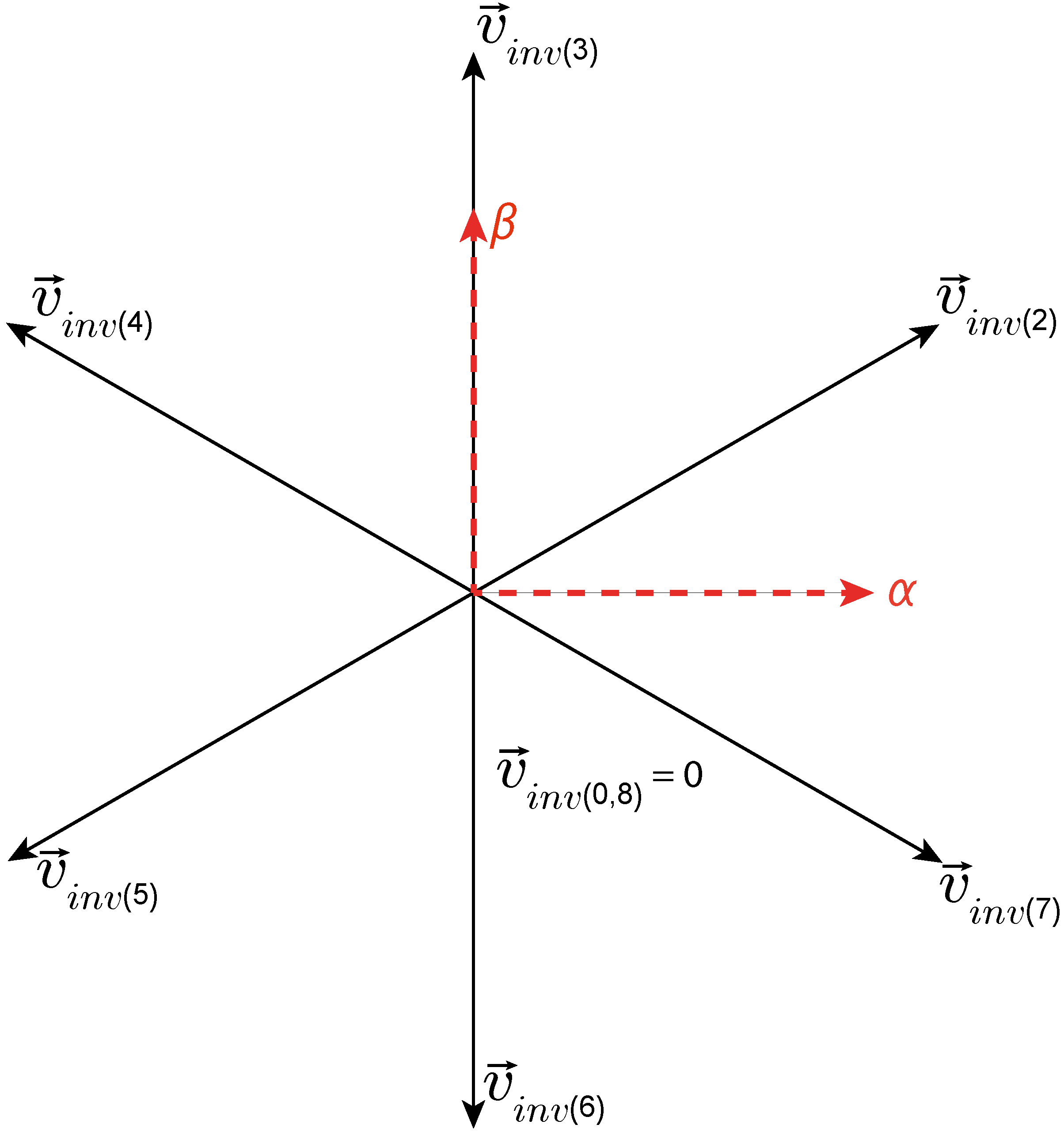
5. Three Vector Modulation (TVM)
The first cost function that should be solved for each pair of vectors corresponding to the sextant in
Figure 2 and
Table 1 is (
19).
Figure 2 refers to the voltage vectors available for the VSI in the
plane.
Figure 2 is divided into six sectors with their related two adjacent vectors; the first sector, as an example, is between vector
and vector
presented in
Table 1 and their respective voltage generated vectors.
Based on the classical predictive control method,
Figure 1 presents a method that uses the same prediction of the load current indicated in (
10). In addition to the main contribution, the proposed techniques use two active vectors in order to maintain a fixed switching frequency. For this to be achieved it is necessary to solve the predictive cost functions separately.
First, the cost function
is solved for each vector existing in VSI according to
Table 1. As an example, for sector II, the cost function is evaluated for both vectors
and
based on (
10) that will change according to the grid voltage. Finally, the duty cycle for each vector is calculated by solving:
where
is the duty cycle of a null vector (
or
) that must be solved only once;
and
are the duty cycles for the adjacent vectors referring to the sector chosen by the algorithm. The duty cycle unit in this case is seconds (
s), as the sampling time (
) is equal to the sum of the duty cycles so that the entire switching period has some voltage vector selected. It is possible to obtain the equation for
K solving the system of (
20), and they are presented below:
From the predicted actions of the power employing Equation (
10), the cost function is calculated in order to select the voltage vectors of the inverter that allows the modulated MPC-FCS as presented before:
where
and
are the cost function with minor values and
and
are the duty clyces computed using Equation (
23).
6. Results Obtained in Experimental Setup
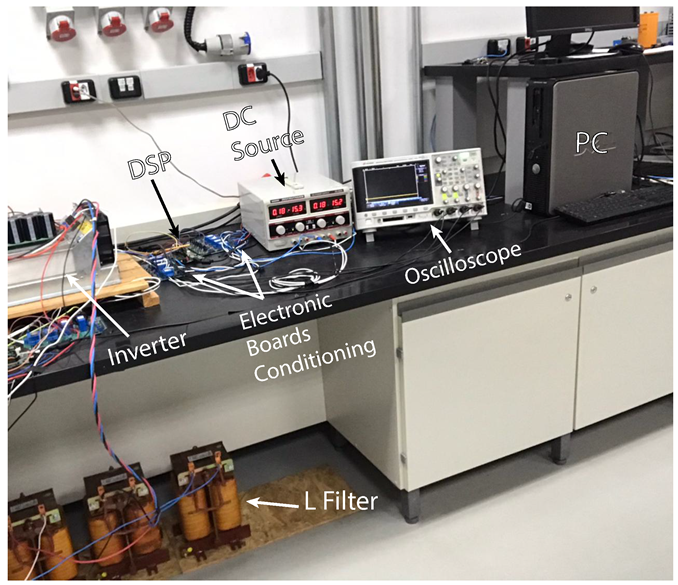
Figure 3 presents the experimental workbench used to evaluate the proposed grid current control using the control robust strategy, which is composed of electronic boards to acquire the voltage (
v) and current (
i) variables, a digital signal processor (DSP) Texas Instruments model TMS320F28335 to implement the controller proposed here and a back-to-back inverter of the model “Semikron SKS20F (B6CI)2P+E1CIF+B6U 14V12” connected to the grid. The parameters of the system are presented in
Table 2.
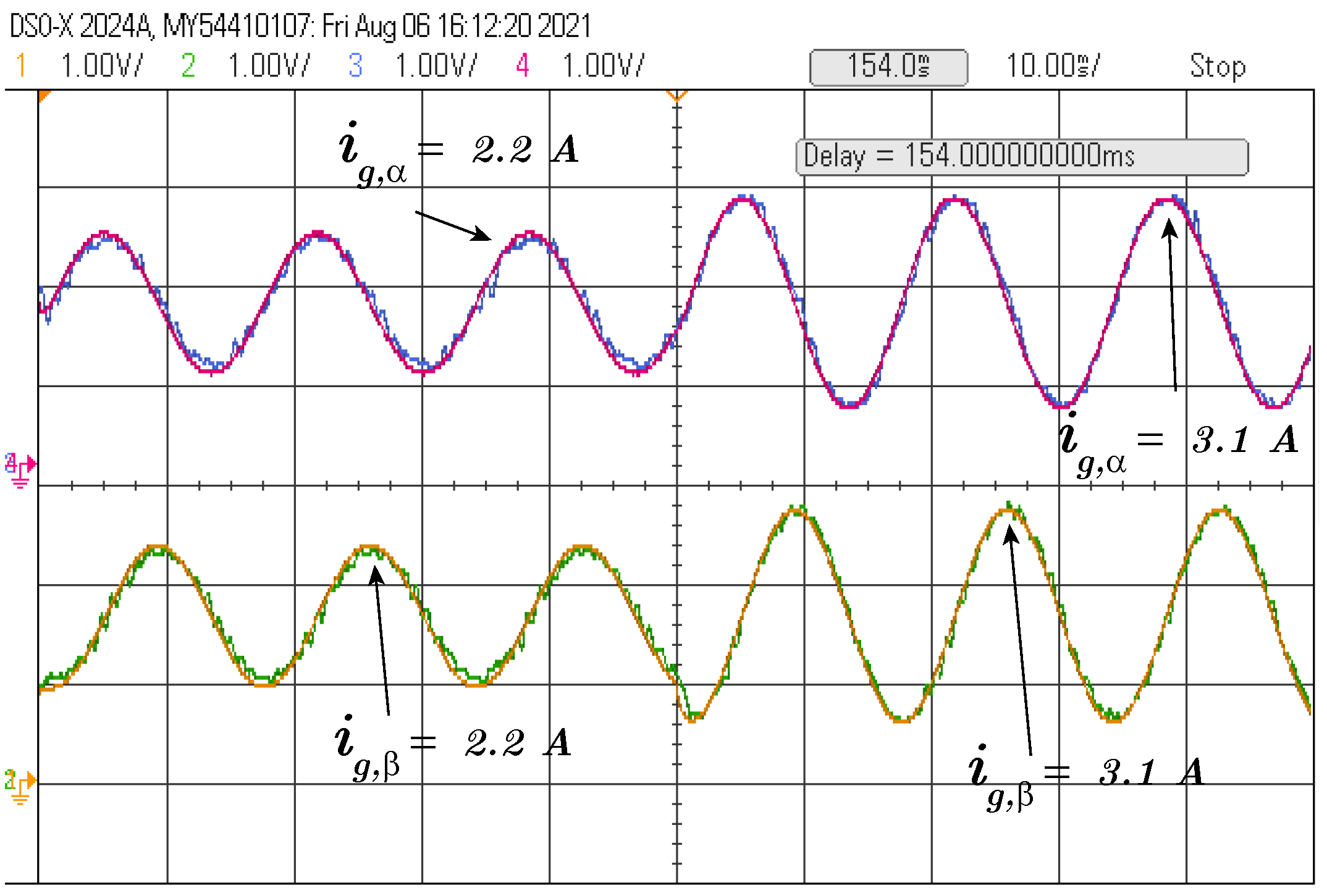
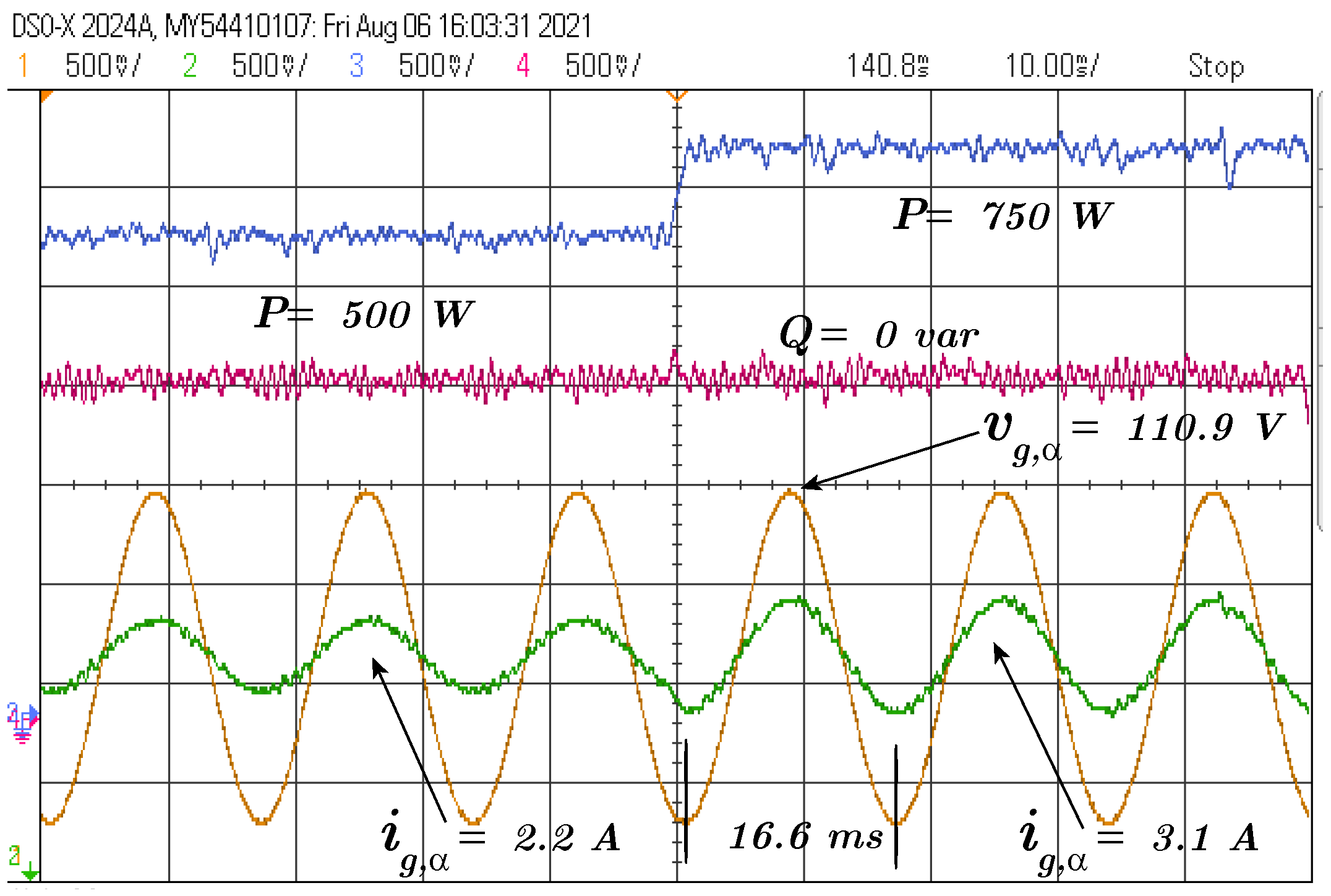
6.1. Results Obtained in Experimental Setup
The first tests were carried out using a degree of active power from 500 W to 750 W with a focus on analyses of the current
and the reference. Notice that the controller is capable of tracking the reference successfully and there is little oscillation around the reference.
Figure 4 presents this first test.
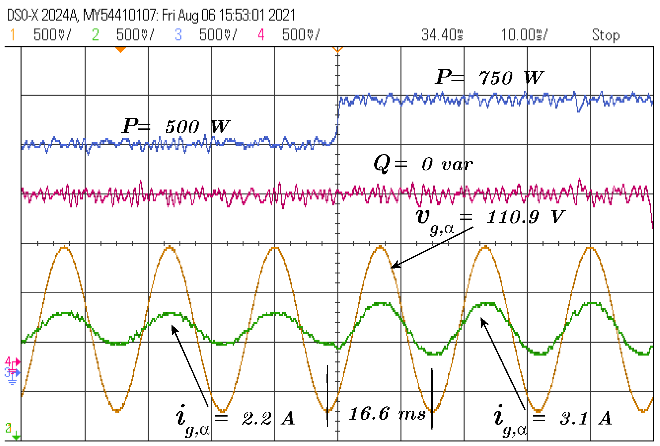
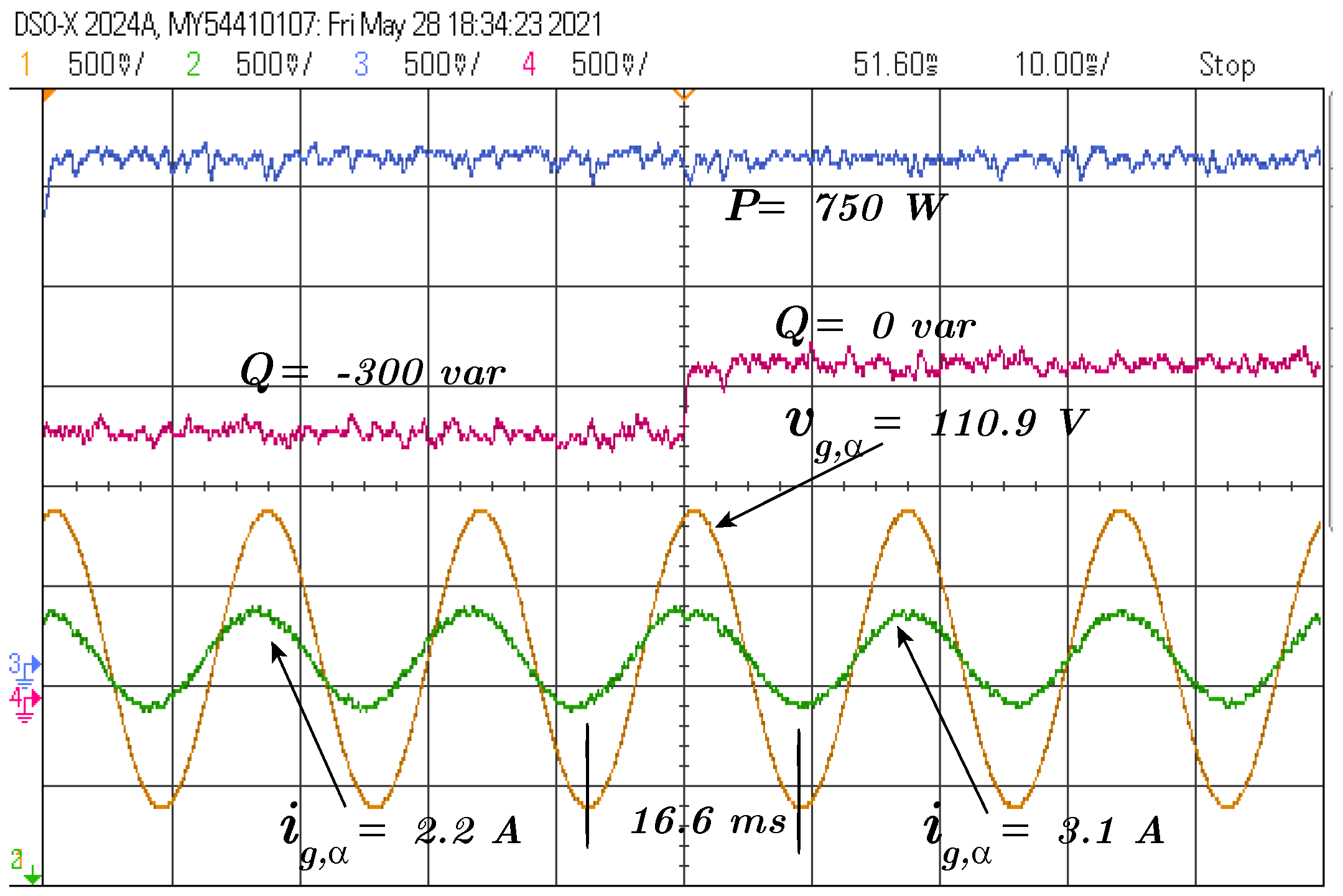
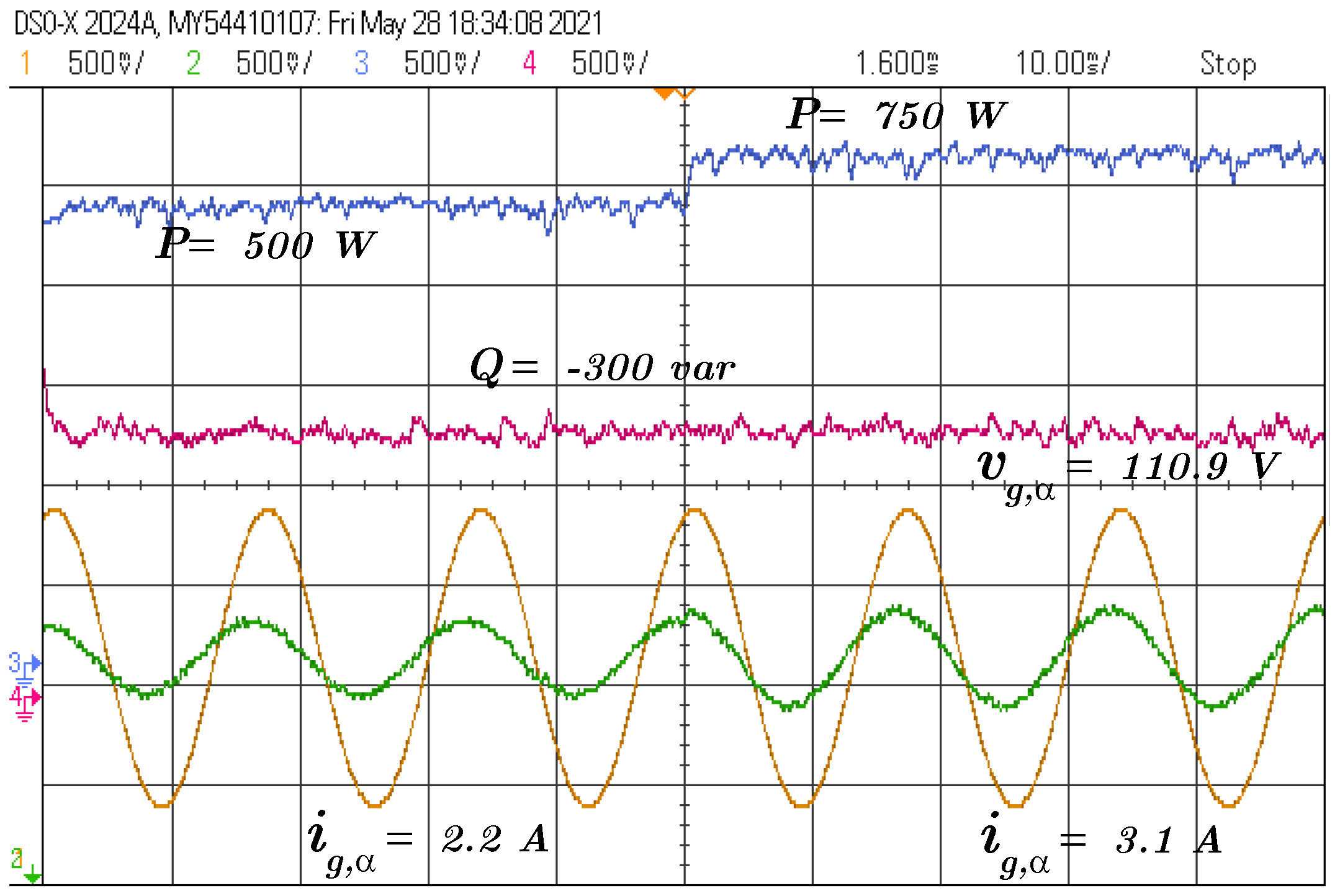
The second test is performed with the same degree of active power, but now it is presented in
Figure 5 with the active and reactive power together with the voltage and current signal.
The following test is a step of reactive power reference
from
var to 0 var, and the active power reference
is maintained at 750 W, as depicted in
Figure 6.
All the tests performed in this subsection present the controller in normal operation connected to the grid. It is noted that the performance of the controller presents satisfactory results and produces a quality current. The following subsections will approach the parameter variation to demonstrate the controller robustness and the total harmonic distortion (THD) to evaluate the quality current injected to the grid.
6.2. Current Test Performance Parameter Variation
This subsection presents the experimental test for parameter variation. The test consists of the parameter change from
to
in five steps, increasing
in each step.
Figure 7 depicts the (
) current under parameter variation.
Notice that even under parameter variation, the current signal maintains a sinusoidal shape; the quality is affected but the controller is still capable of tracking the reference. The next subsection will present a fixed parameter variation to make a deeper analysis of the dynamic response and the quality of the current signal injected into the grid.
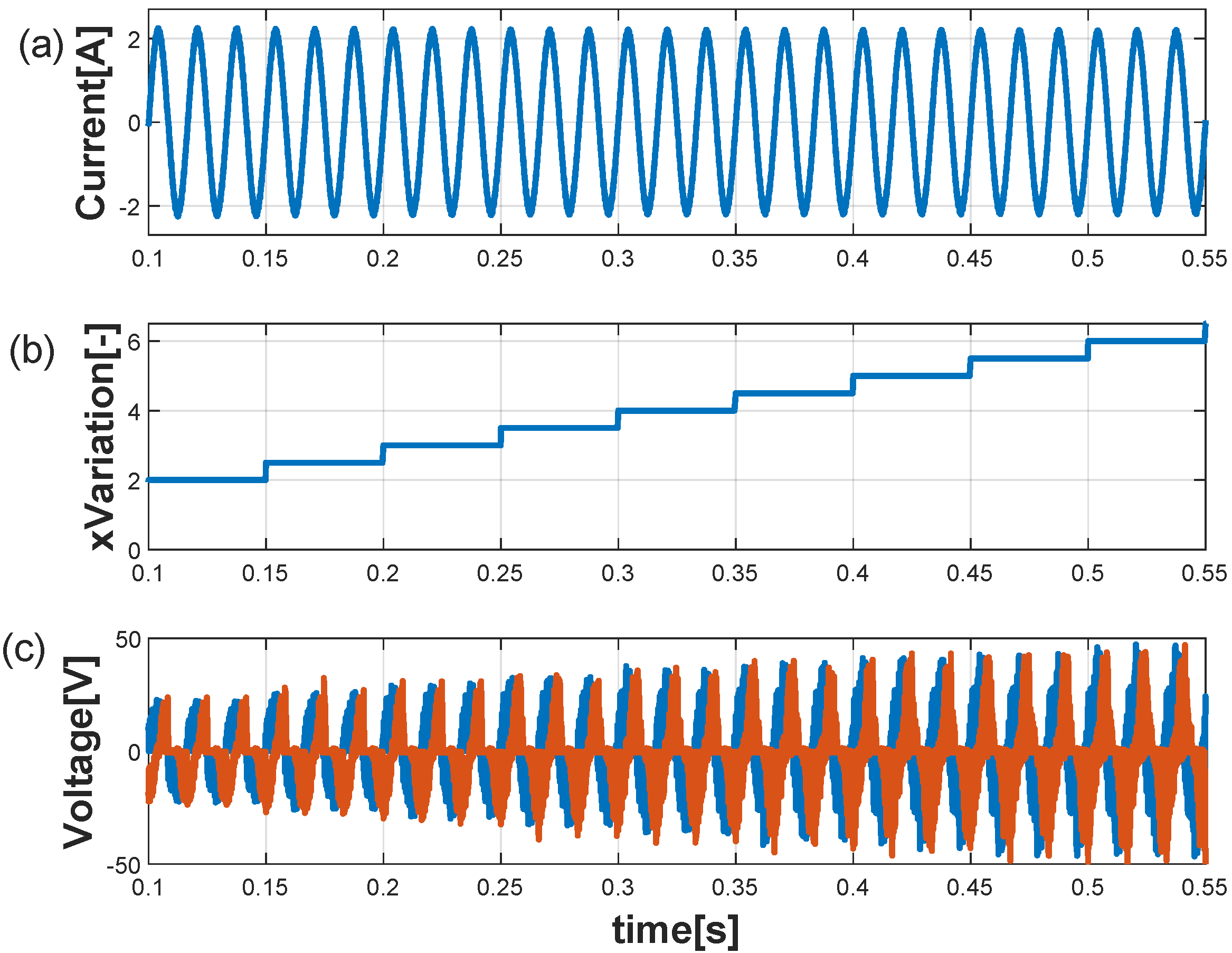
Figure 8 presents a simulation of the controller proposed in MATALB for a variation from 100% to 600%. In addition to the alpha current (
), the robust plots are presented, demonstrating that as a variation appears between the plant and the estimated model, this plot increases and compensates for the variation.
6.3. Test as 160% of Nominal Parameter
This subsection focuses on observing the behavior of the proposed control with
increase of inductance and resistance.
Figure 9 shows the current and the reference under parameter variation.
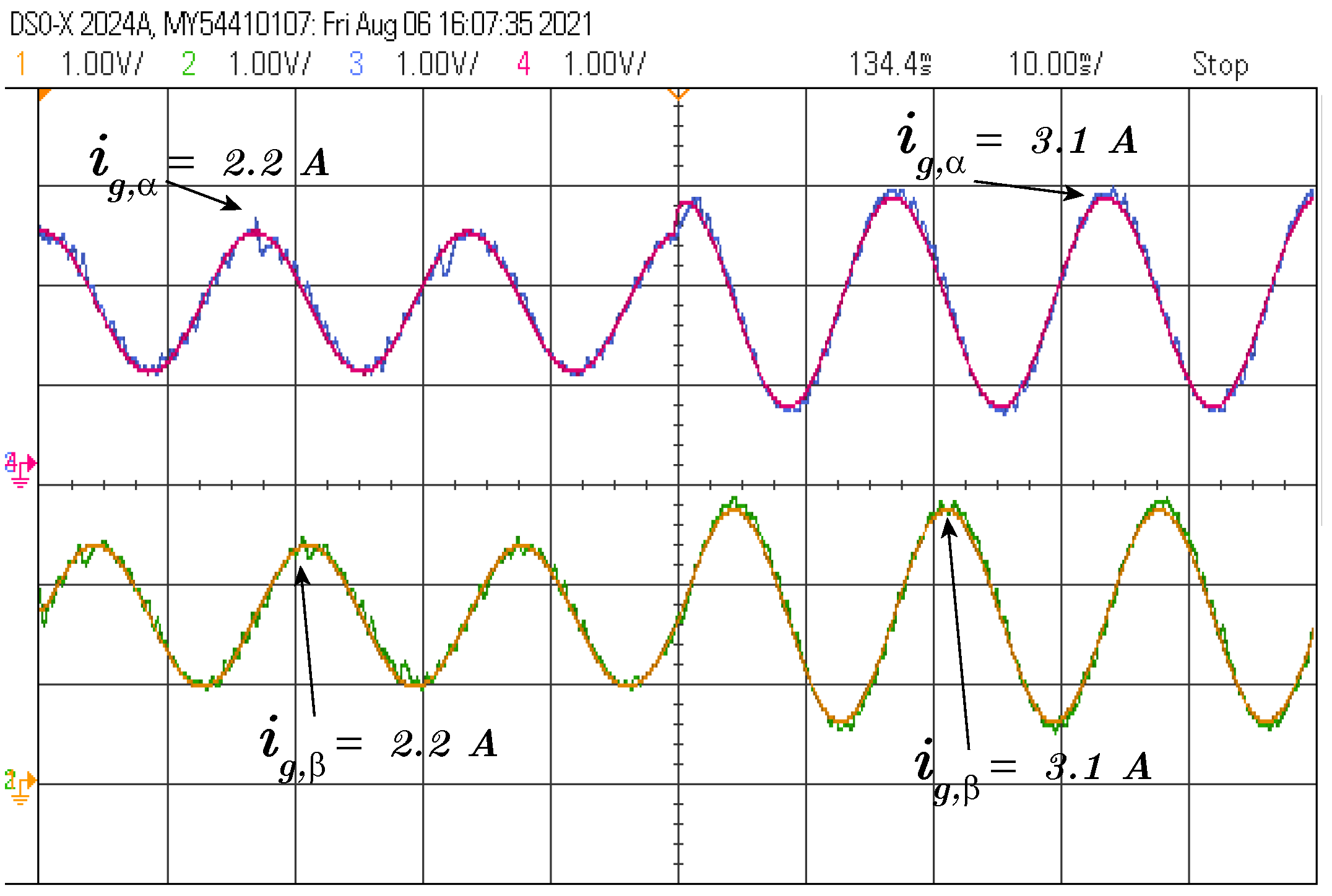
It is possible to observe that the controller achieves the reference; however, it is also noticeable that there is a small increase in the oscillation around the reference due to the variation in the parameters. The next result in
Figure 10 presents the same test in
Figure 5, but now the inductance and the reference are increased by
.
The dynamic response of the system is apparently not affected, as observed in
Figure 10. To obtain a deeper analysis of the result, the CSV data were extracted and plotted using MATLAB to observe the details and the comparison between the system in normal operation and the operation under parameter variation.
This comparison is presented in
Figure 11. To represent a 60% increase in the parameter value, the ×1.6 multiplier (blue line) was used, in the same way the ×1.0 multiplier (red line) represents the parameters in nominal values.
Notice that in both cases the rise time is approximately
ms. This value of dynamic response is considered good when compared to the same dynamic response presented in [
30]. The only visible difference is in the fact that there is a different minimum stationary error in the two cases due to the variation of the parameters, but still not enough to affect the system performance. The result supports the idea that the proposed controller is capable of maintaining the system dynamic response even under parameter variation.
Figure 12 presents the dynamic response from the CSV data obtained through the test bench for MPC and the RFCS to illustrate the performance for both controllers. For the same test conditions, the RFCS achieved
ms and the MPC
ms, which demonstrates the acceptable dynamic response for the proposed controller.
6.4. Test as 60% of Nominal Parameter
To evaluate the behavior of the system when the inductance is 40%,
Figure 13 presents the system response with the variation. It is noticeable that there is greater noise reproduced in the systems because, with a smaller inductance, the filter has a smaller effect on the system, and the switching noise is less attenuated. However, even with the variation of the parameters, the system still operates efficiently.
6.5. Total Harmonic Distortion (THD)
To analyze the quality of current injected to the grid, the CSV data obtained by the experimental test was used to plot the THD graphic using MATLAB tools.
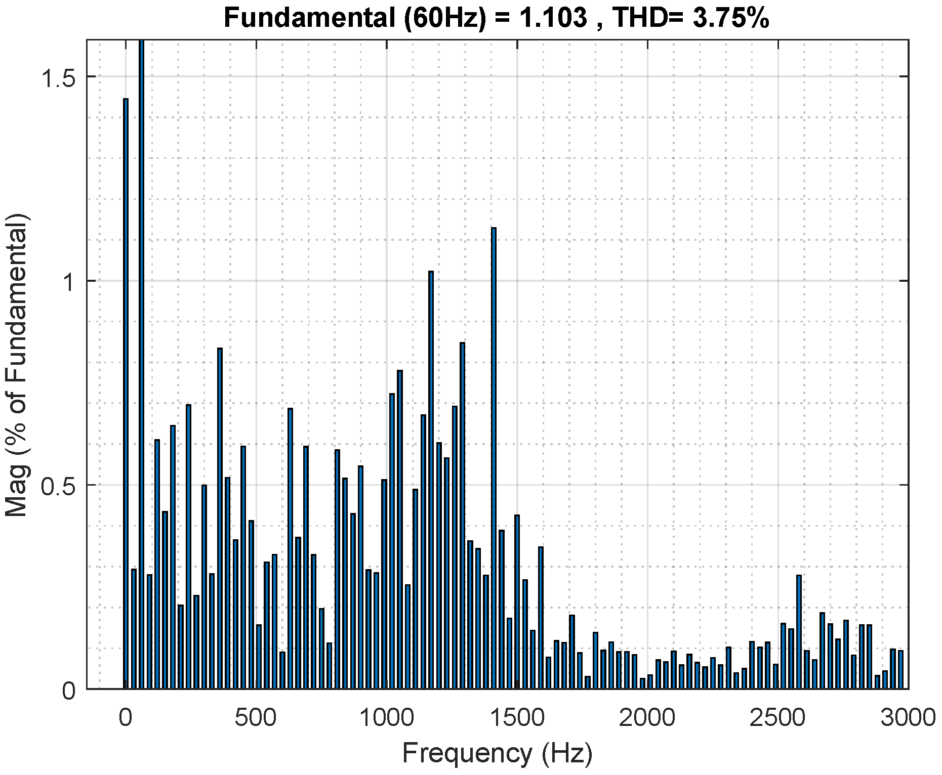
Figure 14 presents the THD result for the current produced by the system in normal operation.
The THD result for the current is
, in accordance with the grid requirements of IEEE Std 1547.2-2008 [
24], for which it is necessary to be below
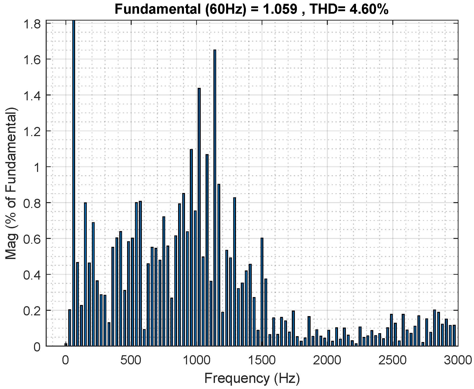
. The next THD analysis is for the current with the system under parameter variation, for which the resistance and inductance were increased in
, presented in
Figure 15.
Notice that the THD value increases to , but it is still in accordance with IEEE Std 1547.2-2008. To conclude the evaluation about the quality of current injected to the grid in both cases, normal operation and parameter variation, the controller is robust enough to produce the current under , which is required by the standard.
7. Conclusions
A predictive robust controller and its practical implementation were presented in the article. To evaluate the controller performance, dynamic response analyses and THD graphics were presented. The methodology to implement the proposed controller step by step was presented in each section. Furthermore, the mathematical elaboration of the robust portion and plant modeling were also presented so the reader can understand the theory used to elaborate the controller. The proposal is based on the robust controllers handling systems with possible parameter variation, which is a daily problem for control systems.
The experimental results of the system connected to the grid show that the rise time for normal operation and under parameter variation have almost the same values, approximately ms, with no overshoot and a low stationary error. The robustness of the controller was validated when the results for normal operation and under parameter variation were still in accordance with IEEE Std 1547.2-2008 for current injected to the grid.
Finally, it is conclusive that this proposed controller has great performance, which makes it eligible for energy application for solar or wind energy systems, which are the trends for environmentally friendly systems. The biggest disadvantage of the controller that should be highlighted is that it is a limited controller in its prediction and control horizons, being only a prediction step in the present proposed control. For future work, it may be possible to change the predictive controller to another type that uses the state-space model and other control and prediction horizons.


 ,
, 


