Vertical Dynamic Impedance of a Viscoelastic Pile in Arbitrarily Layered Soil Based on the Fictitious Soil Pile Model

Abstract

The vertical vibration of a viscoelastic pile immersed in arbitrarily layered soil is investigated by taking the interaction among pile, pile surrounding soil (PSS) and pile end soil (PES) into account. Firstly, considering both the stratification and stress wave effect of soil, a mathematical model of the pile–soil system is established based on the fictitious soil pile (FSP) model. Then, utilizing the impedance function transfer method and Laplace transform technique, the analytical solutions of the vertical dynamic impedance of pile are derived in the frequency domain. The analytical solutions are validated by comparing them with other existing solutions. Finally, a parametric study is put forward to investigate the properties of PES on the vertical dynamic impedance of pile. The results reveal that the properties of PES have a significant effect on the vertical dynamic impedance of pile, but there is a critical influence thickness for this effect. For the cases of the PES thickness exceeding the critical influence thickness, further increase of PES thickness will not affect the dynamic behavior of the pile–soil system.

1. Introduction

The vibration theory of pile foundation is the theoretical basis for the dynamic design of the foundations of wind turbines, bridges and other facilities, which has received extensive attention from scholars in the past few decades [1,2,3,4]. Throughout the development of the vibration theory of pile foundation, it can be seen that the pile–soil dynamic interaction models are alwaysthe main line of research regarding the vibration problems of pile foundation. In the field of the dynamic interaction between pile and PSS, there are three typical models, namely, the dynamic Winkler model [5,6,7,8,9,10,11,12,13], plain-strain model [14,15,16,17,18,19,20,21,22] and three-dimensional axisymmetric continuum model [23,24,25,26,27,28,29,30,31,32,33,34]. These models greatly promote the development of pile foundation dynamics. It can be concluded that the types of interaction models between pile and PES are very rich and complex, and the various characteristics of PSS that can be considered are also relatively comprehensive [35].

As it is well known, like the influencing factors of pile bearing capacity, the vibration behavior of pile is also controlled by the interaction among pile, PSS and PES, and the higher the end bearing ratio, the greater the effect of PES [36]. Many research results have also shown that the bearing conditions of PES have an important effect on the dynamic behavior of the pile–soil system. For example, the support stiffness of PES directly determines the vertical and torsional resonance frequencies of pile head, which are little affected by PSS [37,38,39]. Therefore, in many engineering cases, PES would be the main control factor of pile vibration characteristics. Studying and accurately reflecting on itseffect, the vibration characteristics of pile foundation are very important to the development of the vibration theory of pile foundation. However, due to the difficulty of establishing a strict coupling model for the dynamic interaction of pile and its end soil, the research on the effect of PES on the vibration behavior of pile is still insufficient. Through literature research, it is found that two typical models are the most widely utilized. The first one is the rigid model, which assumes the PES to be a fixed boundary [6,14,23,25,26,30,33,35]. The rigid model is only suitable for end-bearing piles. The second one is the elastic model (simulated by a linear spring) [12,27,37,38] or viscoelastic model (simulated by a Voigt model) [7,9,10,11,17,18,19,21,39]. Although these models are convenient to use in engineering, the values of model parameters are mostly determined by an empirical formula, which lacks connection with the PES properties.

In recent years, to overcome the deficiencies of the existing support models of pile bottom, Wu et al. [40] put forward the FSP model where the soil column between the pile end and the bedrock (i.e., the soil column within the projection range of the pile cross-section) is regarded as a ‘soil pile’. The parameters of the ‘soil pile’ take the parameters of actual soil layers, and its deformation is assumed to conform to the plane section assumption. In view of the small deformation of the bedrock, the bottom boundary of FSP can be regarded as a rigid boundary. According to the layered characteristics of the PES and whether there is sediment or compaction at the pile end, FSP can be divided into several sections along the vertical direction; that is, the layered characteristics of the PES can be considered in the FSP model. In recent years, the FSP model was also utilized to study the torsional vibration and settlement problems of pile foundation [22,29,41,42,43,44,45]. However, to popularize the model in engineering, the FSP model needs to be applied to more engineering cases to verify its rationality.

In light of this, this paper introduces the FSP model to study the vertical vibration problem of a viscoelastic pile by taking both the stratification and stress wave effect of soil into account. Firstly, the vertical vibration model of the pile–soil system is established by utilizing the FSP model and a simplified dynamic interaction model between adjacent soil layers [41]. Then, the analytical solutions for the vertical dynamic impedance of pile are derived in the frequency domain by adopting the Laplace transform technique and impedance function transfer method. The present solutions are verified by comparing with some existing simplified answers. Finally, a parametric study is also put forward to study the effect of the properties of PES on the vertical dynamic impedance of pile. The research results of this paper can provide theoretical support for the dynamic design of pile–soil systems considering the strict coupling interaction among pile, PSS and PES. The present model can also provide reference ideas for other complex vibration problems of the pile–soil system.

2. Mathematical Model Construction

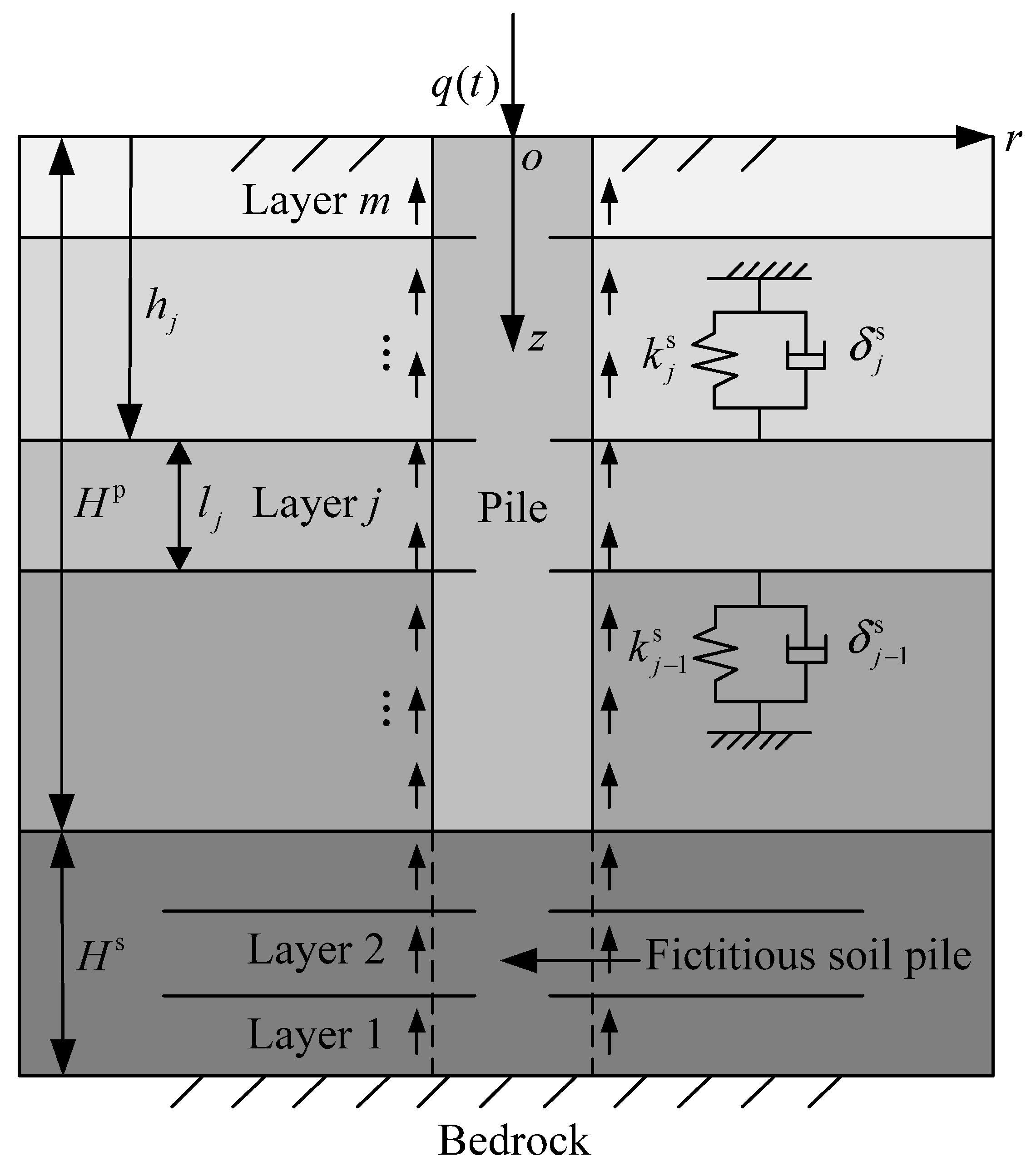
2.1. Geometry of Pile–Soil System

In this paper, the vertical vibration behavior of a viscoelastic pile immersed in arbitrary layered soil is studied based on the FSP model. The stress wave effect of soil in the vertical direction is considered, and the viscoelastic pile is rigorous coupled with its surrounding soil and end soil. The geometry of the pile–soil interaction model is illustrated in Figure 1. Considering the layered characteristics of soil and the variation of the properties (i.e., modulus or sectional area) of pile, the pile–soil system is decomposed into a total of m segments (layers), which are marked by 1, 2, …, j, …, m from the FSP bottom to pile head. $l_j$ and $h_j$ denote the thickness and top surface depth of the jth ($1\le j\le m$) pile–soil segment, respectively. The properties of the pile and soil layer are assumed to be homogeneous within each segment or layer, respectively, but may vary from segment to segment or layer to layer [40]. The radius of the jth pile segment (including FSP) is defined as $r_j^{\mathrm{p}}$. $H^{\mathrm{p}}$ and $H^{\mathrm{s}}$ represent the length of pile shaft and the thickness of PES, respectively. The vertical harmonic force acting on the pile head can be expressed as $q(t)$.

The main assumptions of this paper are given as follows:

(1) The soil surrounding and the underlying pile is viscoelastic, infinite in the radial direction and arbitrarily layered in the vertical direction. The viscous damping coefficient of the jth soil layer is represented by ${\eta }_j^{\mathrm{s}}$ which is in direct proportion to velocity.

(2) There are no normal or shear stresses at the top surface of the soil. The bottom of the PES is the bedrock which can be regarded as a rigid boundary.

(3) The dynamic interaction between adjacent soil layers can be simulated as a distributed Voigt model [41]. The spring constant and damping coefficient of the distributed Voigt model between the jth soil layer and its upper adjacent soil layer can be defined as $k_j^{\mathrm{s}}$ and ${\delta }_j^{\mathrm{s}}$, and the corresponding parameters between the jth soil layer and its lower adjacent soil layer can be denoted by $k_{j-1}^{\mathrm{s}}$ and ${\delta }_{j-1}^{\mathrm{s}}$, respectively.

(4) The stress wave effect of PSS in the vertical direction is considered, and the radial displacement of PSS can be ignored during the vibration of the pile–soil system.

(5) The pile (including FSP) is vertical, viscoelastic and circular in cross-section. During vibration, the pile and PSS, pile and PES are in continuous contact, which results in the stress and displacement at the interface of pile and soil being continuous.

(6) During vibration, the deformations and strains of the whole pile–soil system are relatively small.

2.2. Dynamic Equilibrium Equations of the Pile–Soil System

The vertical displacement of the jth soil layer at any point corresponding to time t is denoted as $w_j=w_j(r,z,t)$. Based on the viscoelastic dynamic theory, the dynamic equilibrium equations of the jth soil layer undergoing vertical axisymmetric excitation about the z-axis of a cylindrical polar coordinate system can be derived as:

$$\begin{array}{l}({\lambda }_j^{\mathrm{s}}+2G_j^{\mathrm{s}})\frac{{\partial }^2{w}_j}{\partial z^2}+G_j^{\mathrm{s}}(\frac{1}{r}\frac{\partial w_j}{\partial r}+\frac{{\partial }^2{w}_j}{\partial r^2})+{\eta }_j^{\mathrm{s}}\frac{\partial }{\partial t}(\frac{{\partial }^2{w}_j}{\partial z^2})+\\ {\eta }_j^{\mathrm{s}}\frac{\partial }{\partial t}(\frac{1}{r}\frac{\partial w_j}{\partial r}+\frac{{\partial }^2{w}_j}{\partial r^2})={\rho }_j^{\mathrm{s}}\frac{{\partial }^2{w}_j}{\partial t^2}\end{array}$$

(1)

where ${\lambda }_j^{\mathrm{s}}$ and $G_j^{\mathrm{s}}$ are the Lame’s constants of the jth soil layer and satisfy ${\lambda }_j^{\mathrm{s}}=E_j^{\mathrm{s}}{\mu }_j^{\mathrm{s}}/[(1+{\mu }_j^{\mathrm{s}})(1-2{\mu }_j^{\mathrm{s}})]$ and $G_j^{\mathrm{s}}={\rho }_j^{\mathrm{s}}{(V_j^{\mathrm{s}})}^2$, respectively; $E_j^{\mathrm{s}}$, ${\rho }_j^{\mathrm{s}}$, $V_j^{\mathrm{s}}$ and ${\mu }_j^{\mathrm{s}}$ are the elastic modulus, density, shear wave velocity and Poisson’s ratio of the jth soil layer, respectively. For the viscoelastic soil, the vertical shear stress amplitude at an arbitrary point in the jth soil layer can be expressed as:

$${\tau }_{rzj}^{\mathrm{s}}=G_j^{\mathrm{s}}\frac{\partial w_j}{\partial r}+{\eta }_j^{\mathrm{s}}\frac{{\partial }^2{w}_j}{\partial t\partial r}$$

(2)

Introducing the Euler–Bernoulli theory, the dynamic equilibrium equations of the jth pile (including FSP) segment can be founded as:

$$E_j^{\mathrm{p}}{A}_j^{\mathrm{p}}\frac{{\partial }^2{u}_j}{\partial z^2}+A_j^{\mathrm{p}}{\eta }_j^{\mathrm{p}}\frac{{\partial }^3{u}_j}{\partial t\partial z^2}-m_j^{\mathrm{p}}\frac{{\partial }^2{u}_j}{\partial t^2}-2\mathsf{\pi }{r}_j^{\mathrm{p}}{\tau }_{rzj}^{\mathrm{s}}(r_j^{\mathrm{p}},z,t)=0$$

(3)

where $u_j=u_j(z,t)$ represents the vertical displacement of the jth pile (including FSP) segment. ${\tau }_{rzj}^{\mathrm{s}}(r_j^{\mathrm{p}},z,t)$ denotes the per unit area shear stress of the jth soil layer acting on the pile shaft at the interface of the pile–soil system. $E_j^{\mathrm{p}}$, ${\eta }_j^{\mathrm{p}}$, $m_j^{\mathrm{p}}$ and $A_j^{\mathrm{p}}$ denote the elastic modulus, viscous damping coefficient, unit mass and cross-section area of the jth pile (including FSP) segment.

2.3. Boundary Conditions (BCs) and Initial Conditions (ICs)

Based on the basic assumptions, the BCs and ICs of the pile-soil system can be obtained in the global coordinate system.

(1) BCs for the jth soil layer can be given as:

At the top surface of the jth soil layer:

$$E_j^{\mathrm{s}}{\frac{\partial w_j}{\partial z}|}_{z=h_j}={(k_j^{\mathrm{s}}{w}_j+{\delta }_j^{\mathrm{s}}\frac{\partial w_j}{\partial t})|}_{z=h_j}$$

(4)

At the bottom surface of the jth soil layer:

$$E_j^{\mathrm{s}}{\frac{\partial w_j}{\partial z}|}_{z=h_j+l_j}=-{(k_{j-1}^{\mathrm{s}}{w}_j+{\delta }_{j-1}^{\mathrm{s}}\frac{\partial w_j}{\partial t})|}_{z=h_j+l_j}$$

(5)

As $r\to \infty$, the shear stress and bounded displacement of the jth soil layer can be written as:

$${\sigma }_j(\infty ,z)=0;\hspace{1em}{w}_j(\infty ,z)=0$$

(6)

(2) BCs for the jth pile (including FSP) segment can be given as:

At the top surface of the jth pile segment:

$${\frac{\partial u_j}{\partial z}|}_{z=h_j}=-{\frac{Z_j^{}(s)u_j}{E_j^{\mathrm{p}}{A}_j^{\mathrm{p}}}|}_{z=h_j}$$

(7)

At the bottom surface of the jth pile segment:

$${\frac{\partial u_j}{\partial z}|}_{z=h_j+l_j}=-{\frac{Z_{j-1}^{}(s)u_j}{E_j^{\mathrm{p}}{A}_j^{\mathrm{p}}}|}_{z=h_j+l_j}$$

(8)

where $Z_{j-1}^{}(s)$ and $Z_j^{}(s)$ represent the vertical dynamic impedance at the bottom and top surface of the jth pile segment, respectively.

(3) BCs at the interface of the pile–soil system can be expressed as:

$$w(r_j^{\mathrm{p}},z,t)=u_j(z,t)$$

(9)

(4) ICs of the pile–soil system can be built as:

The ICs of the jth soil layer:

$${w_j|}_{t=0}=0;\hspace{1em}{\frac{\partial w_j}{\partial t}|}_{t=0}=0;\hspace{1em}{\frac{{\partial }^2{w}_j}{\partial t^2}|}_{t=0}=0$$

(10)

The ICs of the jth pile segment:

$${u_j|}_{t=0}=0;\hspace{1em}{\frac{\partial u_j}{\partial t}|}_{t=0}=0$$

(11)

3. Solutions of Pile Surrounding Soil

Denoting $W_j(r,z,s)={\int }_0^{+\infty }{w}_j(r,z,t)e^{-st}\mathrm{d}t$ as the Laplace transform of $w_j(r,z,t)$ with respect to time and combining with the ICs (Equation (10)), applying the Laplace transform (two-sided) to Equation (1) yields:

$$({\lambda }_j^{\mathrm{s}}+2G_j^{\mathrm{s}}+{\eta }_j^{\mathrm{s}}\cdot s)\frac{{\partial }^2{W}_j}{\partial z^2}+(G_j^{\mathrm{s}}+{\eta }_j^{\mathrm{s}}\cdot s)(\frac{1}{r}\frac{\partial W_j}{\partial r}+\frac{{\partial }^2{W}_j}{\partial r^2})={\rho }_j^{\mathrm{s}}{s}^2{W}_j$$

(12)

where s denotes the Laplace constant.

Applying the separation of variables technique, substituting the single-variable function $W_j(r,z,s)=R_j(r)Z_j(z)$ into Equation (12) gives:

$$\begin{array}{l}({\lambda }_j^{\mathrm{s}}+2G_j^{\mathrm{s}}+{\eta }_j^{\mathrm{s}}\cdot s)\frac{1}{Z_j(z)}\frac{{\partial }^2{Z}_j(z)}{\partial z^2}+\\ (G_j^{\mathrm{s}}+{\eta }_j^{\mathrm{s}}\cdot s)\frac{1}{R_j(r)}(\frac{1}{r}\frac{\partial R_j(r)}{\partial r}+\frac{{\partial }^2{R}_j(r)}{\partial r^2})={\rho }_j^{\mathrm{s}}{s}^2\end{array}$$

(13)

Then, Equation (13) can be divided into the following equations:

$$\frac{{\mathrm{d}}^2{R}_j(r)}{\mathrm{d}{r}^2}+\frac{1}{r}\frac{\mathrm{d}{R}_j(r)}{\mathrm{d}r}-{\xi }_j^2{R}_j(r)=0$$

(14)

$$\frac{{\mathrm{d}}^2{Z}_j(z)}{\mathrm{d}{z}^2}+{\beta }_j^2{Z}_j(z)=0$$

(15)

where ${\xi }_j$ and ${\beta }_j$ are eigenvalues whose relationship is given as:

$$-({\lambda }_j^{\mathrm{s}}+2G_j^{\mathrm{s}}+{\eta }_j^{\mathrm{s}}\cdot s){\beta }_j^2+(G_j^{\mathrm{s}}+{\eta }_j^{\mathrm{s}}\cdot s){\xi }_j^2={\rho }_j^{\mathrm{s}}{s}^2$$

(16)

Equation (16) can be further rewritten as:

$${\xi }_j^2=\frac{({\lambda }_j^{\mathrm{s}}+2G_j^{\mathrm{s}}+{\eta }_j^{\mathrm{s}}\cdot s){\beta }_j^2+{\rho }_j^{\mathrm{s}}{s}^2}{G_j^{\mathrm{s}}+{\eta }_j^{\mathrm{s}}\cdot s}$$

(17)

The general solutions of Equations (14) and (15) can be derived as:

$$R_j(r)=A_j{\mathrm{K}}_0({\xi }_{j}r)+B_j{\mathrm{I}}_0({\xi }_{j}r)$$

(18)

$$Z_j(z)=C_j\sin ({\beta }_{j}z)+D_j\cos ({\beta }_{j}z)$$

(19)

where ${\mathrm{I}}_0(\cdot )$ and ${\mathrm{K}}_0(\cdot )$ are the modified Bessel functions of order zero of the first and second kinds, respectively. $A_j$, $B_j$, $C_j$ and $D_j$ are undetermined constants that can be obtained by utilizing boundary conditions.

Combining Equations (18) and (19), the general solution of Equation (13) can be derived as:

$$W_j(r,z,s)=[A_j{\mathrm{K}}_0({\xi }_{j}r)+B_j{\mathrm{I}}_0({\xi }_{j}r)][C_j\sin ({\beta }_{j}z)+D_j\cos ({\beta }_{j}z)]$$

(20)

The local coordinate system is established for mathematical convenience. To realise that, the global coordinate is transferred into m local coordinates, the origins of which are set at the top surface of each pile segment, and the z-axis of the local coordinate system coincides with that of the global coordinate system. Then, $z=h_j$ and $z=h_j+l_j$ in the global system are transferred to $z^{\prime }=0$ and $z^{\prime }=l_j$ in the local coordinate system, respectively. Taking the Laplace transform of boundary conditions (Equations (4) and (5)) yields:

$$[\frac{(k_j^{\mathrm{s}}+{\delta }_j^{\mathrm{s}}\cdot s)}{E_j^{\mathrm{s}}}{W}_j(r,z^{\prime },s)-{\frac{\partial W_j(r,z^{\prime },s)}{\partial z^{\prime }}]|}_{z^{\prime }=0}=0$$

(21)

$$[\frac{(k_{j-1}^{\mathrm{s}}+{\delta }_{j-1}^{\mathrm{s}}\cdot s)}{E_j^{\mathrm{s}}}{W}_j(r,z^{\prime },s)+{\frac{\partial W_j(r,z^{\prime },s)}{\partial z^{\prime }}]|}_{z^{\prime }=l_j}=0$$

(22)

$${\overline{\sigma }}_j(\infty ,z^{\prime })=0;\hspace{1em}{W}_j(\infty ,z^{\prime })=0$$

(23)

Based on the particular characters of Bessel function as $r\to \infty$, ${\mathrm{I}}_n(\cdot )\to \infty$, ${\mathrm{K}}_n(\cdot )\to 0$ with boundary condition (Equation (23)), the value of $B_j$ can be obtained as: $B_j=0$. Combining Equations (21) and (22) yields:

$$\tan ({\beta }_j{l}_j)=\frac{(\frac{k_j^{\mathrm{s}}+{\delta }_j^{\mathrm{s}}\cdot s}{E_j^{\mathrm{s}}}{l}_j+\frac{k_{j-1}^{\mathrm{s}}+{\delta }_{j-1}^{\mathrm{s}}\cdot s}{E_j^{\mathrm{s}}}{l}_j){\beta }_j{l}_j}{{({\beta }_j{l}_j)}^2-(\frac{k_j^{\mathrm{s}}+{\delta }_j^{\mathrm{s}}\cdot s}{E_j^{\mathrm{s}}}{l}_j)(\frac{k_{j-1}^{\mathrm{s}}+{\delta }_{j-1}^{\mathrm{s}}\cdot s}{E_j^{\mathrm{s}}}{l}_j)}=\frac{({\overline{K}}_j+{\overline{K}}_j{}^{\prime }){\beta }_j{l}_j}{{({\beta }_j{l}_j)}^2-{\overline{K}}_j{\overline{K}}_j{}^{\prime }}$$

(24)

where ${\overline{K}}_j=\frac{k_j^{\mathrm{s}}+{\delta }_j^{\mathrm{s}}\cdot s}{E_j^s}{l}_j$ and ${\overline{K}}_j{}^{\prime }=\frac{k_{j-1}^{\mathrm{s}}+{\delta }_{j-1}^{\mathrm{s}}\cdot s}{E_j^s}{l}_j$ represent the dimensionless complex stiffness at the top and bottom surface of the jth soil layer, respectively. Substituting $s=\mathrm{i}\omega$ into the transcendental Equation (24), the eigenvalue ${\beta }_{jn}$ can be obtained by means of the bisection method in the frequency domain, where $\mathrm{i}=\sqrt{-1}$ is the imaginary unit and $\omega =2\mathsf{\pi }f$ is the circular frequency, in which $f$ is the general frequency. Then, substituting ${\beta }_{jn}$ into Equation (17), the corresponding eigenvalue ${\xi }_{jn}$ can be derived.

Then, the general solution of Equation (13) can be written as:

$$W_j(r,z^{\prime },s)=\sum _{n=1}^{\infty }{A}_{jn}{\mathrm{K}}_0({\xi }_{jn}r)\sin ({\beta }_{jn}{z}^{\prime }+{\varphi }_{jn})\hspace{0.17em}$$

(25)

where ${\varphi }_{jn}=\arctan ({\beta }_{jn}{l}_j/{\overline{K}}_j)$, $A_{jn}$ is the undetermined coeffcients which can be derived from the boundary conditions.

Combined with Equation (25), the per unit area shear stress of the jth soil layer acting on the pile shaft can be further expressed as:

$${\tau }_{rzj}^{\mathrm{s}}(r_j^{\mathrm{p}},z^{\prime },s)=(G_j^{\mathrm{s}}+{\eta }_j^{\mathrm{s}}\cdot s)\sum _{n=1}^{\infty }{A}_{jn}{\xi }_{jn}{\mathrm{K}}_1({\xi }_{jn}{r}_j^{\mathrm{p}})\sin ({\beta }_{jn}{z}^{\prime }+{\varphi }_{jn})\hspace{0.17em}$$

(26)

4. Solutions of Pile and Fictitious Soil Pile

4.1. Solutions for the First FSP Segment

Applying the Laplace transform to Equation (3) on both sides and converting the global coordinates to the local coordinates yields:

$$\begin{array}{l}{(V_1^{\mathrm{p}})}^2(1+\frac{{\eta }_1^{\mathrm{p}}}{E_1^{\mathrm{p}}}\cdot s)\frac{{\partial }^2{U}_1}{\partial z^{\prime }{}^2}-s^2{U}_1-\\ \frac{2\mathsf{\pi }{r}_1^{\mathrm{p}}}{{\rho }_1^{\mathrm{p}}{A}_1^{\mathrm{p}}}(G_1^{\mathrm{s}}+{\eta }_1^{\mathrm{s}}\cdot s){\displaystyle \sum _{n=1}^{\infty }{A}_{1n}{\xi }_{1n}{\mathrm{K}}_1({\xi }_{1n}{r}_1^{\mathrm{p}})}\sin ({\beta }_{1n}{z}^{\prime }+{\varphi }_{1n})\hspace{0.17em}=0\end{array}$$

(27)

where $U_1(z,s)$ is the Laplace transform of $u_1(z,t)$ with respect to time, $V_1^{\mathrm{p}}=\sqrt{E_1^{\mathrm{p}}/{\rho }_1^{\mathrm{p}}}$ denotes the one-dimensional elastic longitudinal wave velocity of the first FSP segment. The general solution of homogeneous equation Equation (27) can be obtained as:

$$U_1^{\#}=M_1\cos ({\overline{\lambda }}_1{z}^{\prime }/l_1)+N_1\sin ({\overline{\lambda }}_1{z}^{\prime }/l_1)$$

(28)

where ${\overline{\lambda }}_1$ is the dimensionless eigenvalue, which can be obtained as:

$${\overline{\lambda }}_1=\sqrt{-\frac{s^2{t}_1^2}{1+\frac{{\eta }_1^{\mathrm{p}}}{E_1^{\mathrm{p}}}\cdot s}}$$

(29)

where $t_1=l_1/V_1^{\mathrm{p}}$ is the propagation time of elastic longitudinal wave propagating in the first FSP segment.

Based on the theory of partial differential equations, the particular solution of Equation (27) can be assumed as:

$$U_1^{*}={\displaystyle \sum _{n=1}^{\infty }{\gamma }_{1n}}\sin ({\beta }_{1n}{z}^{\prime }+{\varphi }_{1n})$$

(30)

where,

$${\gamma }_{1n}=-\frac{2\mathsf{\pi }{r}_1^{\mathrm{p}}(G_1^{\mathrm{s}}+{\eta }_1^{\mathrm{s}}\cdot s)A_{1n}{\xi }_{1n}{\mathrm{K}}_1({\xi }_{1n}{r}_1^{\mathrm{p}})}{{\rho }_1^{\mathrm{p}}{A}_1^{\mathrm{p}}[{({\beta }_{1n}{V}_1^{\mathrm{p}})}^2(1+\frac{{\eta }_1^{\mathrm{p}}}{E_1^{\mathrm{p}}}\cdot s)+s^2]}$$

(31)

Combining Equations (28) and (39), the vertical displacement $U_1$ of the first FSP segment can be obtained as:

$$U_1=U_1^{\#}+U_1^{*}=M_1\cos ({\overline{\lambda }}_1{z}^{\prime }/l_1)+N_1\sin ({\overline{\lambda }}_1{z}^{\prime }/l_1)+{\displaystyle \sum _{n=1}^{\infty }{\gamma }_{1n}}\sin ({\beta }_{1n}{z}^{\prime }+{\varphi }_{1n})$$

(32)

Applying the Laplace transform (two-sided) to Equation (9) and combining the displacement continuity condition (Equation (9)) with Equations (25) and (32) yields:

$$\begin{array}{l}{M}_1\cos ({\overline{\lambda }}_1{z}^{\prime }/l_1)+N_1\sin ({\overline{\lambda }}_1{z}^{\prime }/l_1)+{\displaystyle \sum _{n=1}^{\infty }{\gamma }_{1n}}\sin ({\beta }_{1n}{z}^{\prime }+{\varphi }_{1n})=\\ {\displaystyle \sum _{n=1}^{\infty }{A}_{1n}{\mathrm{K}}_0({\xi }_{1n}{r}_1^{\mathrm{p}})}\sin ({\beta }_{1n}{z}^{\prime }+{\varphi }_{1n})\hspace{0.17em}\end{array}$$

(33)

Merging the similar terms, Equation (33) can be reduced as:

$$M_1\cos ({\overline{\lambda }}_1{z}^{\prime }/l_1)+N_1\sin ({\overline{\lambda }}_1{z}^{\prime }/l_1)={\displaystyle \sum _{n=1}^{\infty }{A}_{1n}{\phi }_{1n}}\sin ({\beta }_{1n}{z}^{\prime }+{\varphi }_{1n})\hspace{0.17em}$$

(34)

where,

$${\phi }_{1n}={\mathrm{K}}_0({\xi }_{1n}{r}_1^{\mathrm{p}})+\frac{2\mathsf{\pi }{r}_1^{\mathrm{p}}(G_1^{\mathrm{s}}+{\eta }_1^{\mathrm{s}}\cdot s){\xi }_{1n}{\mathrm{K}}_1({\xi }_{1n}{r}_1^{\mathrm{p}})}{{\rho }_1^{\mathrm{p}}{A}_1^{\mathrm{p}}[{({\beta }_{1n}{V}_1^{\mathrm{p}})}^2(1+\frac{{\eta }_1^{\mathrm{p}}}{E_1^{\mathrm{p}}}\cdot s)+s^2]}$$

(35)

The systems of eigenfunctions $\sin ({\beta }_{1n}{z}^{\prime }+{\varphi }_{1n})\hspace{0.17em}$ are orthogonal over the interval $z=\left[0,l_1\right]$ and satisfy the following relationship:

$$\{\begin{array}{l}{\int }_0^{l_1}\sin ({\beta }_{1n}{z}^{\prime }+{\varphi }_{1n})\hspace{0.17em}\sin ({\beta }_{1m}{z}^{\prime }+{\varphi }_{1m})\hspace{0.17em}\mathrm{d}{z}^{\prime }=0,m\ne n\\ {\int }_0^{l_1}\sin ({\beta }_{1n}{z}^{\prime }+{\varphi }_{1n})\hspace{0.17em}\sin ({\beta }_{1m}{z}^{\prime }+{\varphi }_{1m})\hspace{0.17em}\mathrm{d}{z}^{\prime }\ne 0,m=n\end{array}$$

(36)

Multiplying $\sin ({\beta }_{1k}{z}^{\prime }+{\varphi }_{1k})\hspace{0.17em}$ on Equation (34) (two-sided) and integrating over range $z=\left[0,l_i\right]$ yields:

$$\begin{array}{l}-\frac{M_1}{2}[\frac{\cos [({\beta }_{1n}+\frac{{\overline{\lambda }}_1}{l_1})l_1+{\varphi }_{1n}]-\cos {\varphi }_{1n}}{{\beta }_{1n}+\frac{{\overline{\lambda }}_1}{l_1}}+\frac{\cos [({\beta }_{1n}-\frac{{\overline{\lambda }}_1}{l_1})l_1+{\varphi }_{1n}]-\cos {\varphi }_{1n}}{{\beta }_{1n}-\frac{{\overline{\lambda }}_1}{l_1}}]\\ -\frac{N_1}{2}[\frac{\sin [({\beta }_{1n}+\frac{{\overline{\lambda }}_1}{l_1})l_1+{\varphi }_{1n}]-\sin {\varphi }_{1n}}{{\beta }_{1n}+\frac{{\overline{\lambda }}_1}{l_1}}-\frac{\sin [({\beta }_{1n}-\frac{{\overline{\lambda }}_1}{l_1})l_1+{\varphi }_{1n}]-\sin {\varphi }_{1n}}{{\beta }_{1n}-\frac{{\overline{\lambda }}_1}{l_1}}]\\ =A_{1n}{\phi }_{1n}{\int }_0^{l_1}{\sin }^2({\beta }_{1n}{z}^{\prime }+{\varphi }_{1n})\mathrm{d}{z}^{\prime }\end{array}$$

(37)

To obtain the vertical displacement amplitude of the first FSP segment, substituting Equation (37) into Equation (32) gives:

$$\begin{array}{l}{U}_1=M_1[\cos ({\overline{\lambda }}_1{z}^{\prime }/l_1)+{\displaystyle \sum _{n=1}^{\infty }{\chi }_{1n}^{\prime }}\sin ({\beta }_{1n}{z}^{\prime }+{\varphi }_{1n})\hspace{0.17em}]+\\ N_1[\sin ({\overline{\lambda }}_1{z}^{\prime }/l_1)+{\displaystyle \sum _{n=1}^{\infty }{\chi }_{1n}^{″}}\sin ({\beta }_{1n}{z}^{\prime }+{\varphi }_{1n})\hspace{0.17em}\hspace{0.17em}]\end{array}$$

(38)

where,

$${\chi }_{1n}^{\prime }={\chi }_{1n}[\frac{\cos ({\overline{\beta }}_{1n}+{\overline{\lambda }}_1+{\varphi }_{1n})-\cos {\varphi }_{1n}}{{\overline{\beta }}_{1n}+{\overline{\lambda }}_1}+\frac{\cos ({\overline{\beta }}_{1n}-{\overline{\lambda }}_1+{\varphi }_{1n})-\cos {\varphi }_{1n}}{{\overline{\beta }}_{1n}-{\overline{\lambda }}_1}]$$

(39)

$${\chi }_{1n}^{″}={\chi }_{1n}[\frac{\sin ({\overline{\beta }}_{1n}+{\overline{\lambda }}_1+{\varphi }_{1n})-\sin {\varphi }_{1n}}{{\overline{\beta }}_{1n}+{\overline{\lambda }}_1}-\frac{\sin ({\overline{\beta }}_{1n}-{\overline{\lambda }}_1+{\varphi }_{1n})-\sin {\varphi }_{1n}}{{\overline{\beta }}_{1n}-{\overline{\lambda }}_1}]$$

(40)

$${\chi }_{1n}=\frac{(G_1^{\mathrm{s}}+{\eta }_1^{\mathrm{s}}\cdot s){\overline{\xi }}_{1n}{\mathrm{K}}_1({\overline{\xi }}_{1n}{\overline{r}}_1^{\mathrm{p}})t_1^2}{{\rho }_1^{\mathrm{p}}{l}_1{\overline{r}}_1^{\mathrm{p}}[{\overline{\beta }}_{1n}^2(1+\frac{{\eta }_1^{\mathrm{p}}}{E_1^{\mathrm{p}}}\cdot s)+s^2{t}_1^2]{\phi }_{1n}{L}_{1n}}$$

(41)

$${\phi }_{1n}={\mathrm{K}}_0({\overline{\xi }}_{1n}{\overline{r}}_1^{\mathrm{p}})+\frac{2(G_1^{\mathrm{s}}+{\eta }_1^{\mathrm{s}}\cdot s){\overline{\xi }}_{1n}{\mathrm{K}}_1({\overline{\xi }}_{1n}{\overline{r}}_1^{\mathrm{p}})t_1^2}{{\rho }_1^{\mathrm{p}}{l}_1^2{\overline{r}}_1^{\mathrm{p}}[{\overline{\beta }}_{1n}^2(1+\frac{{\eta }_1^{\mathrm{p}}}{E_1^{\mathrm{p}}}\cdot s)+s^2{t}_1^2]}$$

(42)

$$L_{1n}={\int }_0^{l_1}{\sin }^2({\beta }_{1n}{z}^{\prime }+{\varphi }_{1n})\mathrm{d}{z}^{\prime }$$

(43)

where ${\overline{\beta }}_{1n}={\beta }_{1n}{l}_1$, ${\overline{\xi }}_{1n}={\xi }_{1n}{l}_1$ and ${\overline{r}}_1^{\mathrm{p}}=r_1^{\mathrm{p}}/l_1$ are dimensionless parameters.

The undetermined constants $M_1$ and $N_1$ can be obtained by the BCs for the top and bottom surface of the first FSP segment. Applying the Laplace transform (two-sided) to BCs (Equations (7) and (8)) and converting Equations (7) and (8) from the global coordinates to the local coordinates yields:

$${\frac{\partial U_1}{\partial z^{\prime }}|}_{z^{\prime }=0}=-{\frac{Z_1^{}(s)U_1}{E_1^{\mathrm{p}}{A}_1^{\mathrm{p}}}|}_{z^{\prime }=0}$$

(44)

$${\frac{\partial U_1}{\partial z^{\prime }}|}_{z^{\prime }=l_1}=-{\frac{Z_0^{}(s)U_1}{E_1^{\mathrm{p}}{A}_1^{\mathrm{p}}}|}_{z^{\prime }=l_1}$$

(45)

For the first FSP segment, the bottom can be regarded as a rigid boundary, that is, $Z_0^{}(s)=\infty$. Substituting $Z_0^{}(s)=\infty$ and Equation (38) into Equation (45) yields:

$$\frac{M_1}{N_1}=-\frac{\sin {\overline{\lambda }}_1+{\displaystyle \sum _{n=1}^{\infty }{\chi }_{1n}^{″}}\sin ({\overline{\beta }}_{1n}+{\varphi }_{1n})}{\cos {\overline{\lambda }}_1+{\displaystyle \sum _{n=1}^{\infty }{\chi }_{1n}^{\prime }}\sin ({\overline{\beta }}_{1n}+{\varphi }_{1n})}$$

(46)

Then, substituting Equation (38) into Equation (44) yields:

$$\begin{array}{ll}{Z}_1(s)& =\frac{{-E_1^{\mathrm{p}}{A}_1^{\mathrm{p}}\frac{\partial U_1}{\partial z^{\prime }}|}_{z^{\prime }=0}}{{U_1|}_{z^{\prime }=0}}\\ & =-\frac{E_1^{\mathrm{p}}{A}_1^{\mathrm{p}}}{l_1}\frac{\frac{M_1}{N_1}{\displaystyle \sum _{n=1}^{\infty }{\chi }_{1n}^{\prime }{\overline{\beta }}_{1n}}\cos {\varphi }_{1n}+{\overline{\lambda }}_1+{\displaystyle \sum _{n=1}^{\infty }{\chi }_{1n}^{″}{\overline{\beta }}_{1n}}\cos {\varphi }_{1n}}{\frac{M_1}{N_1}[1+{\displaystyle \sum _{n=1}^{\infty }{\chi }_{1n}^{\prime }\sin {\varphi }_{1n}}]+{\displaystyle \sum _{n=1}^{\infty }{\chi }_{1n}^{″}}\sin {\varphi }_{1n}}\end{array}$$

(47)

Substituting Equation (46) into Equation (47), the analytical solution for the displacement impedance at the top surface of the first FSP segment can be gained.

4.2. Solutions for the Viscoelastic Pile in Arbitrarily Layered Soil

The function of displacement impedance of the jth pile segment head during vibration can be derived by utilizing a similar method for the first FSP segment. Then, the displacement of the jth pile segment head is derived as:

$$\begin{array}{l}{U}_j=M_j[\cos ({\overline{\lambda }}_j{z}^{\prime }/l_j)+{\displaystyle \sum _{n=1}^{\infty }{\chi }_{jn}^{\prime }}\sin ({\beta }_{jn}{z}^{\prime }+{\varphi }_{jn})\hspace{0.17em}]+\\ N_j[\sin ({\overline{\lambda }}_j{z}^{\prime }/l_j)+{\displaystyle \sum _{n=1}^{\infty }{\chi }_{jn}^{″}}\sin ({\beta }_{jn}{z}^{\prime }+{\varphi }_{jn})\hspace{0.17em}\hspace{0.17em}]\end{array}$$

(48)

where,

$${\chi }_{jn}^{\prime }={\chi }_{jn}[\frac{\cos ({\overline{\beta }}_{jn}+{\overline{\lambda }}_j+{\varphi }_{jn})-\cos {\varphi }_{jn}}{{\overline{\beta }}_{jn}+{\overline{\lambda }}_j}+\frac{\cos ({\overline{\beta }}_{jn}-{\overline{\lambda }}_j+{\varphi }_{jn})-\cos {\varphi }_{jn}}{{\overline{\beta }}_{jn}-{\overline{\lambda }}_j}]$$

(49)

$${\chi }_{jn}^{″}={\chi }_{jn}[\frac{\sin ({\overline{\beta }}_{jn}+{\overline{\lambda }}_j+{\varphi }_{jn})-\sin {\varphi }_{jn}}{{\overline{\beta }}_{jn}+{\overline{\lambda }}_j}-\frac{\sin ({\overline{\beta }}_{jn}-{\overline{\lambda }}_j+{\varphi }_{jn})-\sin {\varphi }_{jn}}{{\overline{\beta }}_{jn}-{\overline{\lambda }}_j}]$$

(50)

$${\chi }_{jn}=\frac{(G_j^{\mathrm{s}}+{\eta }_j^{\mathrm{s}}\cdot s){\overline{\xi }}_{jn}{\mathrm{K}}_1({\overline{\xi }}_{jn}{\overline{r}}_j^{\mathrm{p}})t_j^2}{{\rho }_j^{\mathrm{p}}{l}_j{\overline{r}}_j^{\mathrm{p}}[{\overline{\beta }}_{jn}^2(1+\frac{{\eta }_j^{\mathrm{p}}}{E_j^{\mathrm{p}}}\cdot s)+s^2{t}_j^2]{\phi }_{jn}{L}_{jn}}$$

(51)

$${\phi }_{jn}={\mathrm{K}}_0({\overline{\xi }}_{jn}{\overline{r}}_j^{\mathrm{p}})+\frac{2(G_j^{\mathrm{s}}+{\eta }_j^{\mathrm{s}}\cdot s){\overline{\xi }}_{jn}{\mathrm{K}}_1({\overline{\xi }}_{jn}{\overline{r}}_j^{\mathrm{p}})t_j^2}{{\rho }_j^{\mathrm{p}}{l}_j^2{\overline{r}}_j^{\mathrm{p}}[{\overline{\beta }}_{jn}^2(1+\frac{{\eta }_j^{\mathrm{p}}}{E_j^{\mathrm{p}}}\cdot s)+s^2{t}_j^2]}$$

(52)

$$L_{jn}={\int }_0^{l_j}{\sin }^2({\beta }_{jn}{z}^{\prime }+{\varphi }_{jn})\mathrm{d}{z}^{\prime }$$

(53)

where ${\overline{\lambda }}_j=\sqrt{-\frac{s^2{t}_j^2}{1+\frac{{\eta }_j^{\mathrm{p}}}{E_j^{\mathrm{p}}}\cdot s}}$, ${\overline{\beta }}_{jn}={\beta }_{jn}{l}_j$, ${\overline{\xi }}_{jn}={\xi }_{jn}{l}_j$ and ${\overline{r}}_j^{\mathrm{p}}=r_j^{\mathrm{p}}/l_j$ are dimensionless parameters. $t_j=l_j/V_j^{\mathrm{p}}$ denotes the propagation time of elastic longitudinal wave propagating in the jth pile segment.

Based on the BCs (Equations (7) and (8)), the function of displacement impedance of the jth pile segment head can be expressed in the local coordinate system as:

$$\begin{array}{ll}{Z}_j(s)& =\frac{{-E_j^{\mathrm{p}}{A}_j^{\mathrm{p}}\frac{\partial U_j}{\partial z^{\prime }}|}_{z^{\prime }=0}}{{U_j|}_{z^{\prime }=0}}\\ & =-\frac{E_j^{\mathrm{p}}{A}_j^{\mathrm{p}}}{l_j}\frac{\frac{M_j}{N_j}{\displaystyle \sum _{n=1}^{\infty }{\chi }_{jn}^{\prime }{\overline{\beta }}_{jn}}\cos {\varphi }_{jn}+{\overline{\lambda }}_j+{\displaystyle \sum _{n=1}^{\infty }{\chi }_{jn}^{″}{\overline{\beta }}_{jn}}\cos {\varphi }_{jn}}{\frac{M_j}{N_j}(1+{\displaystyle \sum _{n=1}^{\infty }{\chi }_{jn}^{\prime }\sin {\varphi }_{jn}})+{\displaystyle \sum _{n=1}^{\infty }{\chi }_{jn}^{″}}\sin {\varphi }_{jn}}\end{array}$$

(54)

where,

$$\frac{M_j}{N_j}=-\frac{\begin{array}{l}{\displaystyle \sum _{n=1}^{\infty }{\chi }_{jn}^{″}}{\overline{\beta }}_{jn}\cos ({\overline{\beta }}_{jn}+{\varphi }_{jn})+{\overline{\lambda }}_j\cos {\overline{\lambda }}_j+\\ \frac{Z_{j-1}(s)l_j}{E_j^{\mathrm{p}}{A}_j^{\mathrm{p}}}[\sin {\overline{\lambda }}_j+{\displaystyle \sum _{n=1}^{\infty }{\chi }_{jn}^{″}}\sin ({\overline{\beta }}_{jn}+{\varphi }_{jn})]\end{array}}{\begin{array}{l}{\displaystyle \sum _{n=1}^{\infty }{\chi }_{jn}^{\prime }}{\overline{\beta }}_{jn}\cos ({\overline{\beta }}_{jn}+{\varphi }_{jn})-{\overline{\lambda }}_j\sin {\overline{\lambda }}_j+\\ \frac{Z_{j-1}(s)l_j}{E_j^{\mathrm{p}}{A}_j^{\mathrm{p}}}[\cos {\overline{\lambda }}_j+{\displaystyle \sum _{n=1}^{\infty }{\chi }_{jn}^{\prime }}\sin ({\overline{\beta }}_{jn}+{\varphi }_{jn})]\end{array}}$$

(55)

Through the transfer function technique [10], the function of displacement impedance of pile head (i.e., the mth pile segment) is derived in the local coordinate system as:

$$Z_m(s)=\frac{{-E_m^{\mathrm{p}}{A}_m^{\mathrm{p}}\frac{\partial U_m}{\partial z^{\prime }}|}_{z^{\prime }=0}}{{U_m|}_{z^{\prime }=0}}=-\frac{E_m^{\mathrm{p}}{A}_m^{\mathrm{p}}}{l_m}{Z}_m^{\prime }(s)$$

(56)

where $Z_m^{\prime }(s)$ is the dimensionless function of displacement impedance of pile head which can be obtained as:

$$Z_m^{\prime }(s)=\frac{\frac{M_m}{N_m}{\displaystyle \sum _{n=1}^{\infty }{\chi }_{mn}^{\prime }{\overline{\beta }}_{mn}}\cos {\varphi }_{mn}+{\overline{\lambda }}_m+{\displaystyle \sum _{n=1}^{\infty }{\chi }_{mn}^{″}{\overline{\beta }}_{mn}}\cos {\varphi }_{mn}}{\frac{M_m}{N_m}(1+{\displaystyle \sum _{n=1}^{\infty }{\chi }_{mn}^{\prime }\sin {\varphi }_{mn}})+{\displaystyle \sum _{n=1}^{\infty }{\chi }_{mn}^{″}}\sin {\varphi }_{mn}}$$

(57)

where,

$$\frac{M_m}{N_m}=-\frac{\begin{array}{l}{\displaystyle \sum _{n=1}^{\infty }{\chi }_{mn}^{″}}{\overline{\beta }}_{mn}\cos ({\overline{\beta }}_{mn}+{\varphi }_{mn})+{\overline{\lambda }}_m\cos {\overline{\lambda }}_m+\\ \frac{Z_{m-1}(s)l_m}{E_m^{\mathrm{p}}{A}_m^{\mathrm{p}}}[\sin {\overline{\lambda }}_m+{\displaystyle \sum _{n=1}^{\infty }{\chi }_{mn}^{″}}\sin ({\overline{\beta }}_{mn}+{\varphi }_{mn})]\end{array}}{\begin{array}{l}{\displaystyle \sum _{n=1}^{\infty }{\chi }_{mn}^{\prime }}{\overline{\beta }}_{mn}\cos ({\overline{\beta }}_{mn}+{\varphi }_{mn})-{\overline{\lambda }}_m\sin {\overline{\lambda }}_m+\\ \frac{Z_{m-1}(s)l_m}{E_m^{\mathrm{p}}{A}_m^{\mathrm{p}}}[\cos {\overline{\lambda }}_m+{\displaystyle \sum _{n=1}^{\infty }{\chi }_{mn}^{\prime }}\sin ({\overline{\beta }}_{mn}+{\varphi }_{mn})]\end{array}}$$

(58)

$${\chi }_{mn}^{\prime }={\chi }_{mn}[\frac{\cos ({\overline{\beta }}_{mn}+{\overline{\lambda }}_m+{\varphi }_{mn})-\cos {\varphi }_{mn}}{{\overline{\beta }}_{mn}+{\overline{\lambda }}_m}+\frac{\cos ({\overline{\beta }}_{mn}-{\overline{\lambda }}_m+{\varphi }_{mn})-\cos {\varphi }_{mn}}{{\overline{\beta }}_{mn}-{\overline{\lambda }}_m}]$$

(59)

$${\chi }_{mn}^{″}={\chi }_{mn}[\frac{\sin ({\overline{\beta }}_{mn}+{\overline{\lambda }}_m+{\varphi }_{mn})-\sin {\varphi }_{mn}}{{\overline{\beta }}_{mn}+{\overline{\lambda }}_m}-\frac{\sin ({\overline{\beta }}_{mn}-{\overline{\lambda }}_m+{\varphi }_{mn})-\sin {\varphi }_{mn}}{{\overline{\beta }}_{mn}-{\overline{\lambda }}_m}]$$

(60)

$${\chi }_{mn}=\frac{(G_m^{\mathrm{s}}+{\eta }_m^{\mathrm{s}}\cdot s){\overline{\xi }}_{mn}{\mathrm{K}}_1({\overline{\xi }}_{mn}{\overline{r}}_m^{\mathrm{p}})t_m^2}{{\rho }_m^{\mathrm{p}}{l}_m{\overline{r}}_m^{\mathrm{p}}[{\overline{\beta }}_{mn}^2(1+\frac{{\eta }_m^{\mathrm{p}}}{E_m^{\mathrm{p}}}\cdot s)+s^2{t}_m^2]{\phi }_{mn}{L}_{mn}}$$

(61)

$${\phi }_{mn}={\mathrm{K}}_0({\overline{\xi }}_{mn}{\overline{r}}_m^{\mathrm{p}})+\frac{2(G_m^{\mathrm{s}}+{\eta }_m^{\mathrm{s}}\cdot s){\overline{\xi }}_{mn}{\mathrm{K}}_1({\overline{\xi }}_{mn}{\overline{r}}_m^{\mathrm{p}})t_m^2}{{\rho }_m^{\mathrm{p}}{l}_m^2{\overline{r}}_m^{\mathrm{p}}[{\overline{\beta }}_{mn}^2(1+\frac{{\eta }_m^{\mathrm{p}}}{E_m^{\mathrm{p}}}\cdot s)+s^2{t}_m^2]}$$

(62)

$$L_{mn}={\int }_0^{l_m}{\sin }^2({\beta }_{mn}{z}^{\prime }+{\varphi }_{mn})\mathrm{d}{z}^{\prime }$$

(63)

where ${\overline{\lambda }}_m=\sqrt{-\frac{s^2{t}_m^2}{1+\frac{{\eta }_m^{\mathrm{p}}}{E_m^{\mathrm{p}}}\cdot s}}$, ${\overline{\beta }}_{mn}={\beta }_{mn}{l}_m$, ${\overline{\xi }}_{mn}={\xi }_{mn}{l}_m$ and ${\overline{r}}_m^{\mathrm{p}}=r_m^{\mathrm{p}}/l_m$ are dimensionless parameters. $t_m=l_m/V_m^{\mathrm{p}}$ is the propagation time of elastic longitudinal wave propagating in the mth pile segment. ${\varphi }_{mn}$ and ${\beta }_{mn}$ are parameters determined by the following equations:

$${\varphi }_{mn}=\arctan ({\beta }_{mn}{l}_m/{\overline{K}}_m)$$

(64)

$$\tan ({\beta }_m{l}_m)=\frac{({\overline{K}}_m+{\overline{K}}_m{}^{\prime }){\beta }_m{l}_m}{{({\beta }_m{l}_m)}^2-{\overline{K}}_m{\overline{K}}_m{}^{\prime }}$$

(65)

where ${\overline{K}}_m=\frac{k_m^{\mathrm{s}}+{\delta }_m^{\mathrm{s}}\cdot s}{E_m^{\mathrm{s}}}{l}_m$ and ${\overline{K}}_m{}^{\prime }=\frac{k_{m-1}^{\mathrm{s}}+{\delta }_{m-1}^{\mathrm{s}}\cdot s}{E_m^{\mathrm{s}}}{l}_m$ denote the dimensionless complex stiffness at the top and bottom surface of the mth soil layer, respectively. $l_m$ is the thickness of the mth soil layer.

The dimensionless displacement impedance of the pile head is further expressed as:

$$K_d=Z_m^{\prime }(\mathrm{i}\omega )=K+\mathrm{i}C$$

(66)

where the real part $K$ indicates the dynamic stiffness, which reflects the resistance capacity to deformation, and the imaginary part $C$ denotes the dynamic damping reflecting energy consumption.

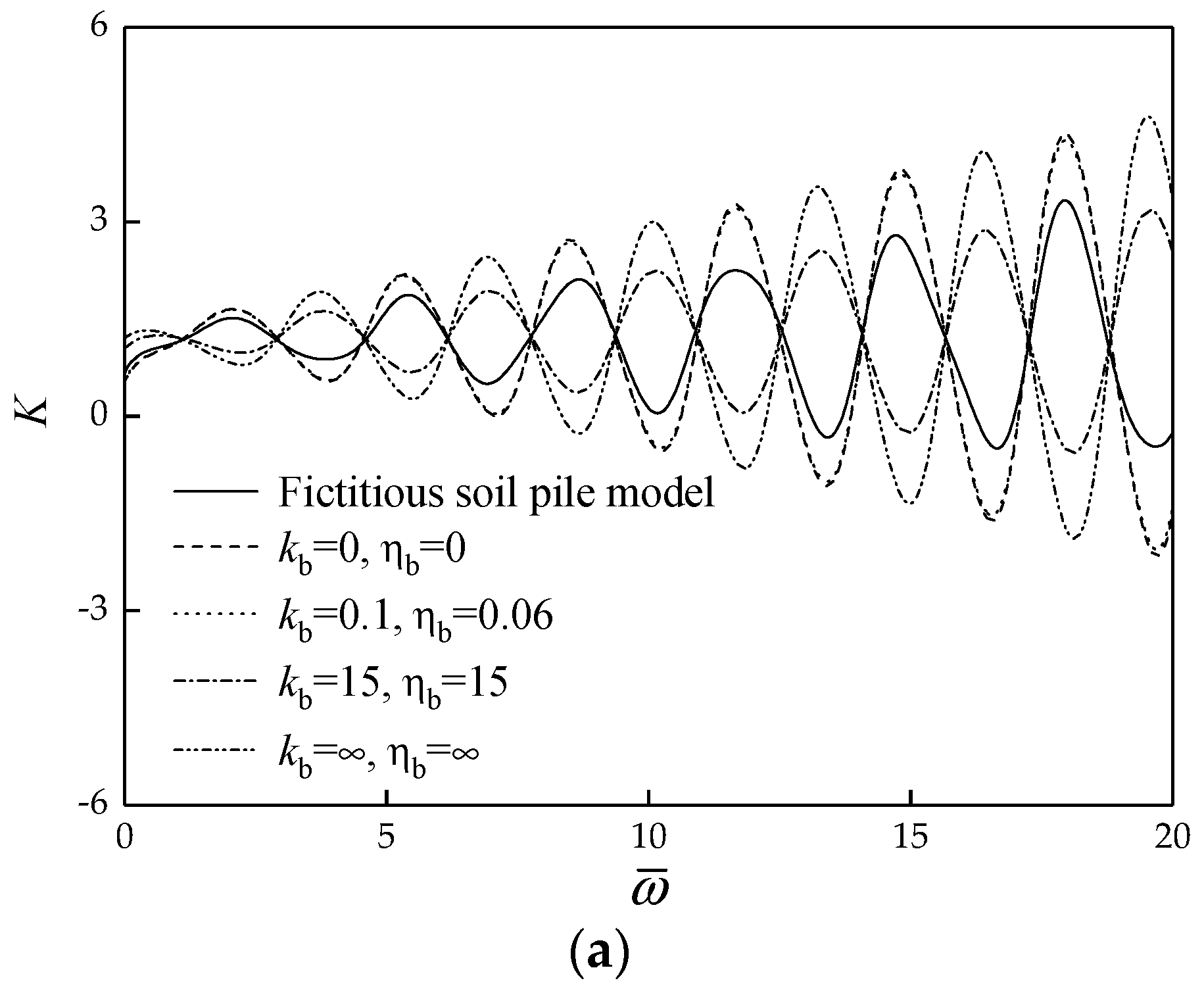
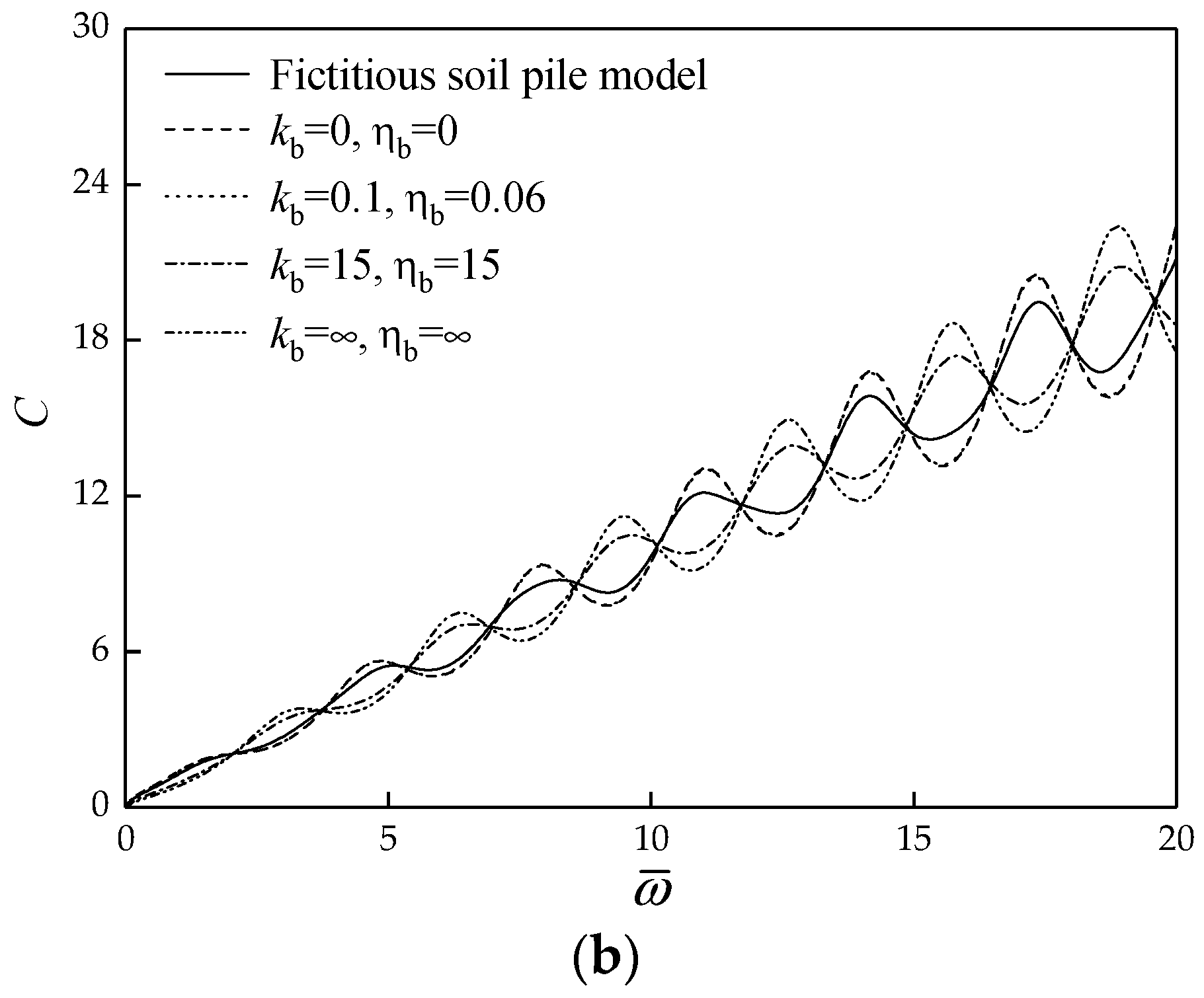
5. Rationality Analysis of the Present Solutions

Through literature research, it is found that the support models of PES to pile are summarized into four categories: ① rigid support, ② free support, ③ viscoelastic support or elastic support and ④ semi-infinite space support. These support models can be generally expressed in the form of complex stiffness $Z_{\mathrm{b}}$, that is:

$$Z_{\mathrm{b}}=k_{\mathrm{b}}+{\delta }_{\mathrm{b}}\cdot \mathrm{i}\omega$$

(67)

where ${\delta }_{\mathrm{b}}$ and $k_{\mathrm{b}}$ denote the damping coefficient and stiffness constant of the support model of pile end, respectively. In the existing literature, many scholars studied the calculation methods of these two parameters. For example, Lysmer and Richart proposed the simulation formula method [46], Novak and Beredugo presented the constant value method [47], Meyerholf obtained the theoretical method of ultimate bearing capacity [48], and Liang and Husein provided the curve equation method [49]. These methods can not consider the thickness and layered properties of PES, which are very empirical. Since the FSP model can consider the thickness and layered properties of PES, it has good application potential in the analysis of dynamic interaction between the pile and its end soil. Next, the FSP model is compared with the existing support models of PES. The calculation parameters are set as: the length, elastic longitudinal wave velocity, density and radius of the pile are 15 m, 3800 $\mathrm{m}/\mathrm{s}$, 2500 ${\mathrm{kg}/\mathrm{m}}^3$ and 0.5 m, respectively. The PES thickness is two times that of the pile diameter. In Figure 2, the different values of $k_{\mathrm{b}}$ and ${\delta }_{\mathrm{b}}$ reflect the other models of the dynamic interaction between pile and PES, namely, $k_{\mathrm{b}}=\infty$ and ${\delta }_{\mathrm{b}}=\infty$ represent rigid support, $k_{\mathrm{b}}=0$ and ${\delta }_{\mathrm{b}}=0$ represent free support, and the other values are viscoelastic support.

Figure 2 illustrate the FSP model with other models. For the viscoelastic support model, the phase difference of resonance frequency between rigid support and free support is 180°, while the resonance frequency obtained by the FSP model is between the calculated results of rigid support and free support. It was also found that the dynamic stiffness and dynamic damping obtained by selecting appropriate material parameters for the FSP model according to the PES properties fall among the calculated values determined by the other existing support models. The result means that the FSP model is reasonable and can be simulated in other models by selecting appropriate parameters of the soil underlying pile end. Furthermore, the FSP model can take the stratification and construction disturbance effect of PES into account, and the parameters of the FSP model can directly take the material parameters of PES without empirical formula calculation. Therefore, the FSP model is more rigorous in theory, for it can more accurately reflect the support effect of PES on pile.

6. Parametric Study

The effect of the PES properties on the vertical dynamic impedance of pile is systemically investigated in this section. Unless otherwise stated, the parameters of the pile–soil system are set as: the length, radius, density and elastic longitudinal wave velocity of the pile are 15 m, 0.5 m, 2500 ${\mathrm{kg}/\mathrm{m}}^3$ and 3800 $\mathrm{m}/\mathrm{s}$, respectively; the density, shear wave velocity, Poisson’s ratio and viscoelastic damping coefficient of PSS are 1800 ${\mathrm{kg}/\mathrm{m}}^3$, 180 $\mathrm{m}/\mathrm{s}$, 0.4 and 1000 $\mathrm{N}\cdot {\mathrm{m}}^{-3}\cdot \mathrm{s}$, respectively. The stiffness constant of the Voigt model between the adjacent soil layers is set as the elastic modulus of the lower soil, and the damping coefficient is set to 10,000 $\mathrm{N}\cdot {\mathrm{m}}^{-3}\cdot \mathrm{s}$ [41].

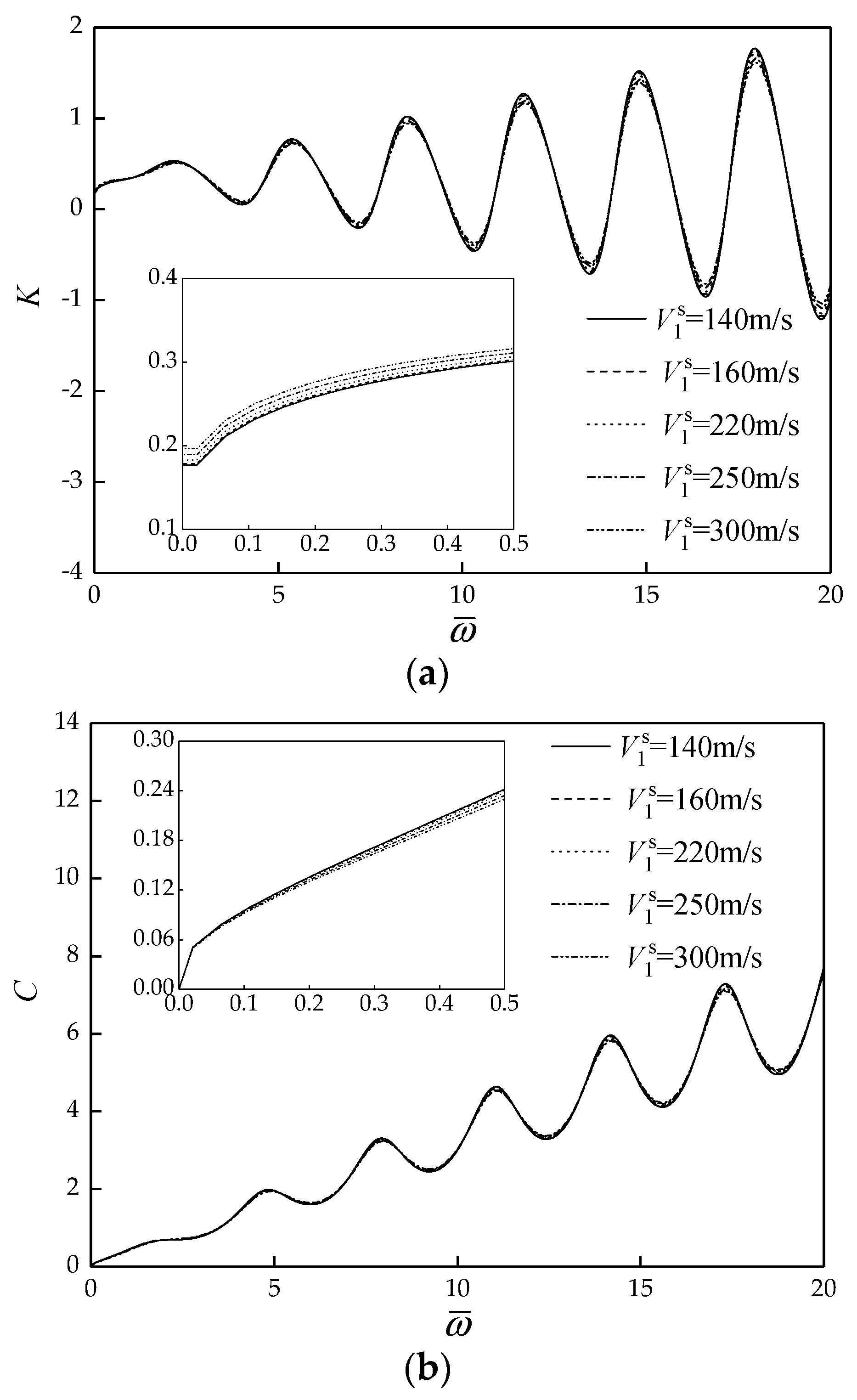
6.1. Effect of Single Homogeneous PES Layer on the Vertical Dynamic Impedance of Pile

In order to more clearly study the effect of PES properties on the vertical dynamic impedance of pile, the cases of a single homogeneous PES layer are analyzed first. In other words, the soil is divided into two layers, i.e., PSS and PES, of which the PES is regarded as homogeneous single media. The density, shear wave velocity, Poisson’s ratio and viscous damping coefficient of PES are 2000 $\mathrm{kg}/{\mathrm{m}}^3$, 220 $\mathrm{m}/\mathrm{s}$, 0.35 and 1000 $\mathrm{N}\cdot {\mathrm{m}}^{-3}\cdot \mathrm{s}$, respectively. $d$ is denoted as the diameter of pile, and the PES thickness can be written as $l_1=0.5d,1d,3d,5d,10d$ when discussing the effect of PES thickness on the vertical dynamic impedance of pile, respectively.

From Figure 3, it can be found that the dynamic stiffness curves and dynamic damping curves trend to convergent with the increase of PES thickness. The result indicates that there is a critical influence depth of PES adjoining to the pile bottom, which has an obvious effect on the vertical dynamic impedance of pile. If the PES thickness exceeds the critical influence thickness, further increase of PES thickness can barely affect the vertical dynamic impedance of pile. Obviously, the vertical dynamic impedance curves of pile should be different for different PES layers. Nevertheless, repeated trial calculation indicates that there is a limited zone of PES which has an effect on the vertical dynamic impedance of pile. In other words, one just needs to focus on the effect of soil properties in a certain range underlying the pile end on the vertical dynamic response of pile.

When discussing the effect of PES shear wave velocity on the vertical dynamic impedance of pile, the density, Poisson’s ratio, viscous damping coefficient, thickness and shear wave velocity of PES are set to 2000 ${\mathrm{kg}/\mathrm{m}}^3$, 0.35, 1000 $\mathrm{N}\cdot {\mathrm{m}}^{-3}\cdot \mathrm{s}$, $3d$ and $V_1^{\mathrm{s}}=140 \mathrm{m}/\mathrm{s},160 \mathrm{m}/\mathrm{s},220 \mathrm{m}/\mathrm{s},250 \mathrm{m}/\mathrm{s},300 \mathrm{m}/\mathrm{s}$, respectively.

Figure 4 display the effect of PES shear wave velocity on the vertical dynamic impedance of pile. It is noted that the formant amplitude in dynamic stiffness curves and dynamic damping curves increases with the decrease of PES shear wave velocity, while the resonant frequency remains basically unchanged. In the low-frequency range which is of interest for dynamic foundation design, the dynamic stiffness of pile gradually increases, and the dynamic damping of pile gradually decreases with the increase of PES shear wave velocity.

When analyzing the effect of PES density on the vertical dynamic impedance of pile, the thickness, shear wave velocity, Poisson’s ratio, viscous damping coefficient and density of PES are $3d$, 220 $\mathrm{m}/\mathrm{s}$, 0.35, 1000 $\mathrm{N}\cdot {\mathrm{m}}^{-3}\cdot \mathrm{s}$, and ${\rho }_1^{\mathrm{s}}={1600 \mathrm{kg}/\mathrm{m}}^3{,1800 \mathrm{kg}/\mathrm{m}}^3{,2000 \mathrm{kg}/\mathrm{m}}^3{,2200 \mathrm{kg}/\mathrm{m}}^3{,2400\mathrm{kg}/\mathrm{m}}^3$, respectively.

Figure 5 indicate the effect of PES density on the vertical dynamic impedance of pile. It is shown that the formant amplitude in dynamic stiffness curves and dynamic damping curves decreases within a small range as the PES density increases. The resonant frequency is hardly affected by the change of PES density. In the low-frequency range which is of interest for dynamic foundation design, the dynamic stiffness of pile gradually increases, and the dynamic damping of pile gradually decreases with the increase of PES density, but the change range is small.

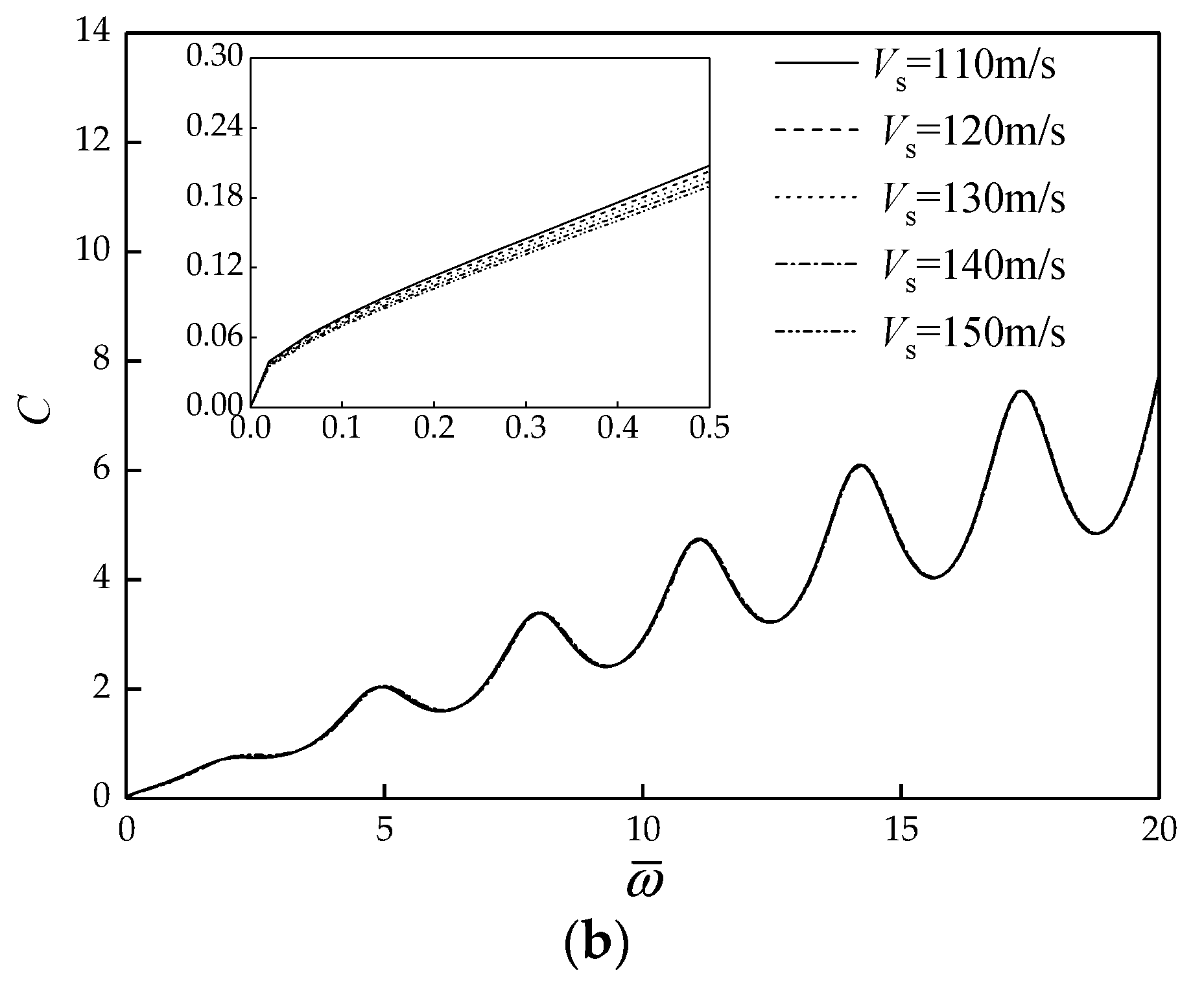
6.2. Effect of Two PES Layers on the Vertical Dynamic Impedance of Pile

In the design of pile foundation, the pile end is usually required to have a certain thickness of bearing stratum, which can ensure that the bearing characteristics of the pile are not affected by the properties of the soil layers below the bearing stratum. In light of this, the effect of soft subsoil below bearing stratum on the vertical dynamic impedance of pile is investigated. The soil is divided into three layers, namely PSS, bearing stratum and soft subsoil from top to bottom. The thickness, density, shear wave velocity, Poisson’s ratio and viscous damping coefficient of bearing stratum are 3 m, 2000 ${\mathrm{kg}/\mathrm{m}}^3$, 220 $\mathrm{m}/\mathrm{s}$, 0.35 and 1000 $\mathrm{N}\cdot {\mathrm{m}}^{-3}\cdot \mathrm{s}$, respectively. The density, shear wave velocity, Poisson’s ratio, viscous damping coefficient and thickness of soft subsoil are 1700 ${\mathrm{kg}/\mathrm{m}}^3$, 100 $\mathrm{m}/\mathrm{s}$, 0.4, 1000 $\mathrm{N}\cdot {\mathrm{m}}^{-3}\cdot \mathrm{s}$ and $l_1=0d,1d,3d,5d,10d$, respectively.

Figure 6 display the effect of thickness of soft subsoil on the vertical dynamic impedance of pile. It is evident that when the bearing stratum is deep enough, the variation of thickness of soft subsoil has little effect on the vertical dynamic impedance of pile. The effects of shear wave velocity and density of soft subsoil on the vertical dynamic impedance of pile are also analyzed in detail, and it is also found that these two parameters basically do not affect the vertical dynamic impedance of pile if the thickness of the bearing stratum is large enough. The figures of the two parameters analysis are not given here because they are basically consistent with Figure 6.

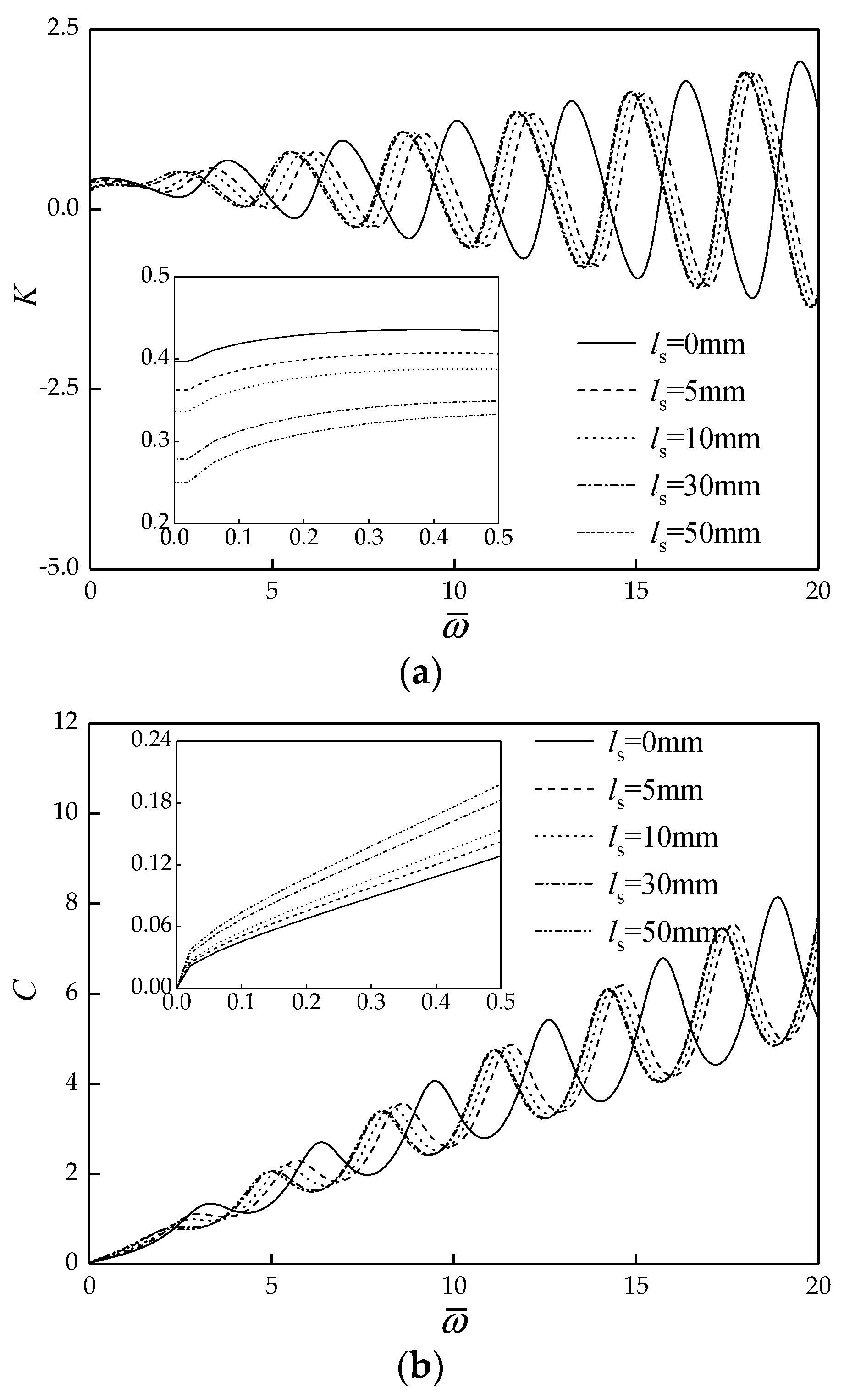
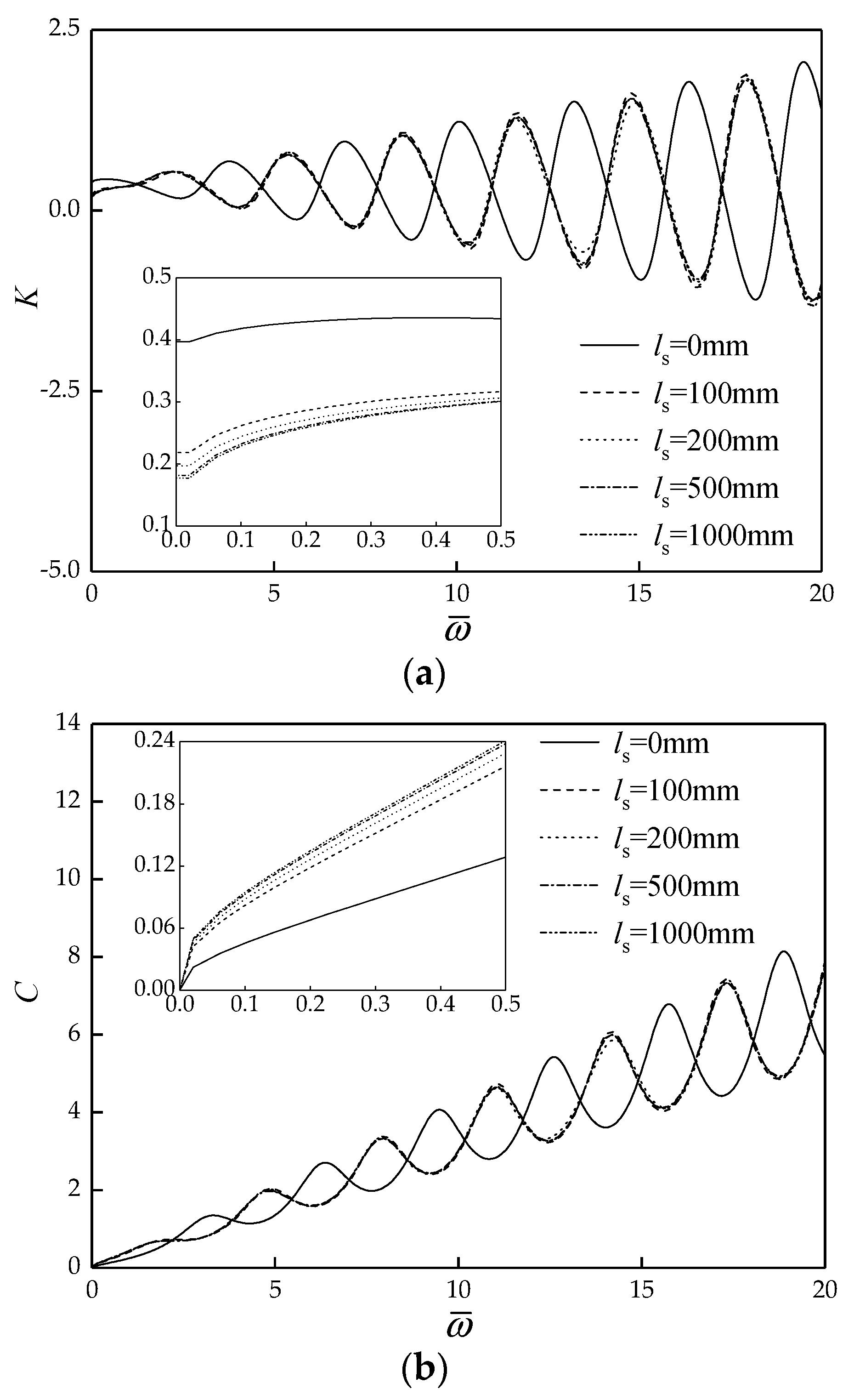
6.3. Effect of Sediment on the Vertical Dynamic Impedance of Rock-Socketed Pile

The rock-socketed pile is the end bearing pile in most cases, and the requirements for the control of sediment at pile end are very high. According to the most commonly related quality acceptance criteria for rock-socketed pile, the thickness of sediment is required to be less than or equal to 50 mm [50]. Therefore, the effect of sediment on the vertical dynamic impedance of rock-socketed pile is discussed for two different engineering conditions. In the first case, the construction quality satisfies acceptance quality, the thickness of sediment is set to: $l_{\mathrm{s}}=0\mathrm{mm},5\mathrm{mm},10\mathrm{mm},30\mathrm{mm},50\mathrm{mm}$, respectively. In the second case, the thickness of sediment is set to an unusual seen value: $l_{\mathrm{s}}=0\mathrm{mm},100\mathrm{mm},200\mathrm{mm},500\mathrm{mm},1000\mathrm{mm}$, respectively, which does not satisfy quality acceptance criteria due to poor construction condition or construction quality. Additionally, the density, shear wave velocity, Poisson’s ratio and viscous damping coefficient of sediment are 1700 ${\mathrm{kg}/\mathrm{m}}^3$, 130 $\mathrm{m}/\mathrm{s}$, 0.4 and 1000 $\mathrm{N}\cdot {\mathrm{m}}^{-3}\cdot \mathrm{s}$, respectively.

The effect of thickness of sediment on the vertical dynamic impedance of rock-socketed pile in case 1 is shown in Figure 7. It can be seen that the thickness of sediment has a remarkable effect on the vertical dynamic impedance of rock-socketed pile. As the thickness of sediment increases, the formant amplitudes of dynamic stiffness curves and damping curves gradually decrease, and the corresponding resonant frequency also gradually becomes smaller, which is a result of the decrease of support stiffness of pile end due to the increase of sediment. In the low frequency, which is of interest in dynamic foundation design, as the sediment thickness increases, the dynamic stiffness of rock-socketed pile decreases, and the dynamic damping of rock-socketed pile increases.

Figure 8 display the effect of thickness of sediment on the vertical dynamic impedance of rock-socketed pile in case 2. It can be seen that the formant amplitude of dynamic stiffness curves and dynamic damping curves decrease within a small scope, and the corresponding resonant frequency has a certain degree of decrease. In the low-frequency range which is of interest in dynamic foundation design, as the sediment thickness increases, the dynamic stiffness of pile head decreases, but the dynamic damping increases. Meanwhile, if the thickness of sediment is more than a threshold, further increase of thickness can hardly give rise to an evident change of the vertical dynamic impedance of rock-socketed pile.

In addition, the effect of the shear wave velocity of sediment on the vertical dynamic impedance of rock-socketed pile is also investigated. The thickness, density, Poisson’s ratio, viscous damping coefficient and shear wave velocity of sediment are 50 mm, 1700 ${\mathrm{kg}/\mathrm{m}}^3$, 0.4, 1000 $\mathrm{N}\cdot {\mathrm{m}}^{-3}\cdot \mathrm{s}$ and $V_{\mathrm{s}}=110 \mathrm{m}/\mathrm{s},120 \mathrm{m}/\mathrm{s},130 \mathrm{m}/\mathrm{s},140 \mathrm{m}/\mathrm{s},150 \mathrm{m}/\mathrm{s}$, respectively.

Figure 9 show the effect of the shear wave velocity of sediment on the vertical dynamic impedance of rock-socketed pile. The formant amplitude of dynamic stiffness and damping barely vary with the increase of shear wave velocity of sediment, but the resonant frequency gradually increases. The results indicate that for the same thickness of sediment, with the increase of shear wave velocity of sediment, the stiffness coefficient of the sediment has a corresponding increase which leads to an increase in the resonant frequency of pile head and the support stiffness of pile toe increases as well. In the low-frequency range which is of interest in dynamic foundation design, with the shear wave velocity of sediment increases, the dynamic stiffness of rock-socketed pile increases, and the dynamic damping of rock-socketed pile decreases.

7. Conclusions

In this paper, the soil adjacent to the pile bottom is simulated by the FSP model, which is perfectly contacted with the pile end. Based on the simplified dynamic interaction between adjacent soil layers, the analytical solutions for the vertical dynamic impedance of pile embedded in arbitrarily layered soil are derived in the frequency domain by means of the Laplace transform technique and impedance function transfer method. Based on the present solutions, a parametric study is conducted to investigate the effect of PES properties on the vertical dynamic impedance of pile. The main conclusions are summarized as follows:

(1) There is a critical influence thickness for the effect of PES thickness on the vertical dynamic impedance of pile. Within the range of critical influence thickness, the variation of the PES thickness has a great effect on the vertical dynamic impedance of pile.

(2) With the improvement of PES, the formant amplitude of the dynamic stiffness curves and dynamic damping curves of pile decreases, but the resonance frequency remains basically unchanged.

(3) In the low-frequency range which is of interest in dynamic foundation design, with the increase of the shear wave velocity and density of PES, the dynamic stiffness of pile gradually increases, and the dynamic damping of pile decreases.

(4) The sediment below the pile end has a remarkable effect on the vertical dynamic impedance of rock-socketed pile. When the thickness of sediment is less than 50 mm, as the thickness of sediment increases, the formant amplitudes of dynamic stiffness curves and damping curves gradually decrease, and the corresponding resonant frequency also gradually becomes smaller.

(5) In the low frequency which is of interest in dynamic foundation design, as the sediment thickness increases, the dynamic stiffness of rock-socketed pile decreases, but the dynamic damping of rock-socketed pile increases.

From the above, it is found that the FSP model is a more rigorous model and has application prospects in engineering practices. In the future, the group of authors will apply the FSP model to investigate the dynamic interaction of pile-soil systems in saturated and unsaturated soils.

References

1. Zhang, H.; Liang, F.Y.; Zheng, H.B. Dynamic impedance of monopiles for offshore wind turbines considering scour-hole dimensions. Appl. Ocean Res. 2021, 107, 102493. [Google Scholar] [CrossRef]
2. Wu, J.T.; El Naggar, M.H.; Zhao, S.; Wen, M.J.; Wang, K.H. Beam-unequal length piles-soil coupled vibrating system considering pile-soil-pile interaction. J. Bridge Eng. 2021, 26, 04021086. [Google Scholar] [CrossRef]
3. Li, L.C.; Zheng, M.Y.; Liu, X.; Wu, W.B.; Liu, H.; El Naggar, M.H.; Jiang, G.S. Numerical analysis of the cyclic loading behavior of monopile and hybrid pile foundation. Comput. Geotech. 2022, 144, 104635. [Google Scholar] [CrossRef]
4. Shao, K.; Su, Q.; Liu, K.W.; Shao, G.X.; Zhong, Z.B.; Li, Z.Q.; Chen, C. A new modified approach to evaluating the installation power of large-diameter helical piles in sand validated by centrifuge and field data. Appl. Ocean Res. 2021, 114, 102756. [Google Scholar] [CrossRef]
5. Novak, M. Vertical vibration of floating pile. J. Eng. Mech. Div. ASCE 1977, 103, 153–168. [Google Scholar] [CrossRef]
6. Nogami, T.; Konagai, K. Time domain axial response of dynamically loaded single piles. J. Eng. Mech. Div. ASCE 1986, 112, 1241–1252. [Google Scholar] [CrossRef]
7. Liao, S.T.; Roesset, J.M. Dynamic response of intact piles to impulse loads. Int. J. Numer. Anal. Met. 1997, 21, 255–275. [Google Scholar] [CrossRef]
8. Michaelides, O.; Gazetas, G.; Bouckovalas, G.; Chrysikou, E. Approximate non-linear dynamic axial response of piles. Geotechnique 1998, 48, 33–53. [Google Scholar] [CrossRef] [Green Version]
9. Militano, G.; Rajapakse, R.K.N.D. Dynamic response of a pile in a multi-layered soil to transient torsional and axial loading. Geotechnique 1999, 49, 91–109. [Google Scholar] [CrossRef]
10. Wang, K.H.; Wu, W.B.; Zhang, Z.Q.; Leo, C.J. Vertical dynamic response of an inhomogeneous viscoelastic pile. Comput. Geotech. 2010, 37, 536–544. [Google Scholar] [CrossRef]
11. Wu, W.B.; El Naggar, M.H.; Abdlrahem, M.; Mei, G.X.; Wang, K.H. New interaction model for vertical dynamic response of pipe piles considering soil plug effect. Can. Geotech. J. 2017, 54, 987–1001. [Google Scholar] [CrossRef]
12. Chen, L.B.; Yang, X.Y.; Wu, W.B.; El Naggar, M.H.; Wang, K.H.; Chen, J.Y. Numerical analysis of the deformation performance of monopile under wave and current load. Energies 2020, 13, 6431. [Google Scholar] [CrossRef]
13. Cui, C.Y.; Liang, Z.M.; Xu, C.S.; Xin, Y.; Wang, B.L.; Meng, K. New Analytical solution to predict the vertical impedance of a large-diameter pipe pile in soil considering wave propagation in visco-elastic continuum. J. Earthq. Tsunami 2021, 2140002. [Google Scholar] [CrossRef]
14. Novak, M. Dynamic stiffness and damping of piles. Can. Geotech. J. 1974, 11, 574–598. [Google Scholar] [CrossRef]
15. Mamoon, S.M.; Banerjee, P.K. Time-domain analysis of dynamically loaded single piles. J. Eng. Mech. Div. ASCE 1992, 118, 140–160. [Google Scholar] [CrossRef]
16. El Naggar, M.H.; Novak, M. Nonlinear lateral interaction in pile dynamics. Soil Dyn. Earthq. Eng. 1995, 14, 141–157. [Google Scholar] [CrossRef]
17. Wu, W.B.; Jiang, G.S.; Huang, S.G.; Mei, G.X.; Leo, C.J. A new analytical model to study the influence of weld on the vertical dynamic response of prestressed pipe pile. Int. J. Numer. Anal. Met. 2017, 41, 1247–1266. [Google Scholar] [CrossRef]
18. Liu, H.; Wu, W.B.; Jiang, G.S.; El Naggar, M.H.; Mei, G.X.; Liang, R.Z. Benefits from using two receivers for the interpretation of low-strain integrity tests on pipe piles. Can. Geotech. J. 2019, 56, 1433–1447. [Google Scholar] [CrossRef]
19. Liu, H.; Wu, W.B.; Yang, X.Y.; Jiang, G.S.; El Naggar, M.H.; Mei, G.S.; Liang, R.Z. Detection sensitivity analysis of pipe pile defects during low-strain integrity testing. Ocean Eng. 2019, 194, 106627. [Google Scholar] [CrossRef]
20. Wu, W.B.; Liu, H.; Yang, X.Y.; Jiang, G.S.; El Naggar, M.H.; Mei, G.S.; Liang, R.Z. New method to calculate apparent phase velocity of open-ended pipe pile. Can. Geotech. J. 2020, 57, 127–138. [Google Scholar] [CrossRef]
21. Zhang, Y.P.; Yang, X.Y.; Wu, W.B.; El Naggar, M.H.; Jiang, G.S.; Liang, R.Z. Torsional complex impedance of pipe pile considering pile installation and soil plug effect. Soil Dyn. Earthq. Eng. 2020, 131, 106010. [Google Scholar] [CrossRef]
22. Guan, W.J.; Wu, W.B.; Jiang, G.S.; Leo, C.J.; Deng, G.D. Torsional dynamic response of tapered pile considering compaction effect and stress diffusion effect. J. Cent. South Univ. 2020, 27, 3839–3851. [Google Scholar] [CrossRef]
23. Nogami, T.; Novak, M. Soil-pile interaction in vertical vibration. Earthq. Eng. Struct. D 1976, 4, 277–293. [Google Scholar] [CrossRef]
24. Rajapakse, R.K.N.D.; Chen, Y.; Senjuntichai, T. Electroelastic field of a piezoelectric annular finite cylinder. Int. J. Solids Struct. 2005, 42, 3487–3508. [Google Scholar] [CrossRef]
25. Wang, K.H.; Zhang, Z.Q.; Leo, C.J.; Xie, K.H. Dynamic torsional response of an end bearing pile in saturated poroelastic medium. Comput. Geotech. 2008, 35, 450–458. [Google Scholar] [CrossRef]
26. Wu, W.B.; Wang, K.H.; Zhang, Z.Q.; Leo, C.J. Soil-pile interaction in the pile vertical vibration considering true three-dimensional wave effect of soil. Int. J. Numer. Anal. Met. 2013, 37, 2860–2876. [Google Scholar] [CrossRef]
27. Luan, L.B.; Ding, X.M.; Zheng, C.J.; Kouretzis, G.; Wu, Q. Dynamic response of pile groups subjected to horizontal loads. Can. Geotech. J. 2020, 57, 469–481. [Google Scholar] [CrossRef]
28. Qu, L.M.; Yang, C.W.; Ding, X.M.; Kouroussis, G.; Zheng, C.J. A continuum-based model on axial pile-head dynamic impedance in inhomogeneous soil. Acta Geotech. 2021, 16, 3339–3353. [Google Scholar] [CrossRef]
29. Cui, C.Y.; Meng, K.; Xu, C.S.; Liang, Z.M.; Li, H.J.; Pei, H.F. Analytical solution for longitudinal vibration of a floating pile in saturated porous media based on a fictitious saturated soil pile model. Comput. Geotech. 2021, 131, 103942. [Google Scholar] [CrossRef]
30. Zhang, Y.P.; Liu, H.; Wu, W.B.; Wang, L.X.; Jiang, G.S. A 3D analytical model for distributed low strain test and parallel seismic test of pipe piles. Ocean Eng. 2021, 225, 108828. [Google Scholar] [CrossRef]
31. Luan, L.B.; Gao, L.; Kouretzis, G.; Ding, X.M.; Qin, H.Y.; Zheng, C.J. Response of pile groups in layered soil to dynamic lateral loads. Comput. Geotech. 2022, 142, 104564. [Google Scholar] [CrossRef]
32. Zheng, C.J.; Cai, Y.J.; Kouretzis, G.; Luan, L.B. Horizontal vibration of rigid strip footings on poroelastic half-space. J. Sound Vib. 2022, 522, 116731. [Google Scholar] [CrossRef]
33. Zhang, Y.P.; Jiang, G.S.; Wu, W.B.; El Naggar, M.H.; Liu, H.; Wen, M.J.; Wang, K.H. Analytical solution for distributed torsional low strain integrity test for pipe pile. Int. J. Numer. Anal. Met. 2022, 46, 47–67. [Google Scholar] [CrossRef]
34. Zhao, M.; Huang, Y.M.; Wang, P.G.; Cao, Y.H.; Du, X.L. An analytical solution for the dynamic response of an end-bearing pile subjected to vertical P-waves considering water-pile-soil interactions. Soil Dyn. Earthq. Eng. 2022, 153, 107126. [Google Scholar] [CrossRef]
35. Wu, W.B.; Yang, Z.J.; Liu, X.; Zhang, Y.P.; Liu, H.; El Naggar, M.H.; Xu, M.J.; Mei, G.X. Horizontal dynamic response of pile in unsaturated soil considering its construction disturbance effect. Ocean Eng. 2022, 245, 110483. [Google Scholar] [CrossRef]
36. Zheng, C.J.; Gan, S.S.; Luan, L.B.; Ding, X.M. Vertical dynamic response of a pile embedded in a poroelastic soil layer overlying rigid base. Acta Geotech. 2021, 16, 977–983. [Google Scholar] [CrossRef]
37. Wu, J.T.; El Naggar, M.H.; Ge, J.; Wang, K.H.; Zhao, S. Multipoint traveling wave decomposition method and its application in extended pile shaft integrity test. J. Geotech. Geoenviron. 2021, 147, 04021128. [Google Scholar] [CrossRef]
38. Yang, D.Y.; Wang, K.H.; Zhang, Z.Q.; Leo, C.J. Longitudinal dynamic response of pile in a radially heterogeneous soil layer. Int. J. Numer. Anal. Met. 2008, 33, 1039–1054. [Google Scholar] [CrossRef]
39. Zhang, Y.P.; Liu, H.; Wu, W.B.; Wang, S.; Wu, T.; Wen, M.J.; Jiang, G.S.; Mei, G.X. Interaction model for torsional dynamic response of thin-wall pipe piles embedded in both vertically and radially inhomogeneous soil. Int. J. Geomech. 2021, 21, 04021185. [Google Scholar] [CrossRef]
40. Wu, W.B.; Wang, K.H.; Ma, S.J.; Leo, C.J. Longitudinal dynamic response of pile in layered soil based on virtual soil pile model. J. Cent. South Univ. 2012, 19, 1999–2007. [Google Scholar] [CrossRef]
41. Wu, W.B.; Jiang, G.S.; Huang, S.G.; Leo, C.J. Vertical dynamic response of pile embedded in layered transversely isotropic soil. Math. Probl. Eng. 2014, 12, 1–12. [Google Scholar] [CrossRef] [Green Version]
42. Wu, W.B.; Liu, H.; El Naggar, M.H.; Mei, G.X.; Jiang, G.S. Torsional dynamic response of a pile embedded in layered soil based on the fictitious soil pile model. Comput. Geotech. 2016, 80, 190–198. [Google Scholar] [CrossRef]
43. Zhang, Y.P.; Wu, W.B.; Jiang, G.S.; Wen, M.J.; Wang, K.H.; El Naggar, M.H.; Ni, P.P.; Mei, G.X. A new approach for estimating the vertical elastic settlement of a single pile based on the fictitious soil pile model. Comput. Geotech. 2021, 134, 104100. [Google Scholar] [CrossRef]
44. Zhang, Y.P.; Wu, W.B.; Zhang, H.K.; El Naggar, M.H.; Wang, K.H.; Jiang, G.S.; Mei, G.X. A novel soil-pile interaction model for vertical pile settlement prediction. Appl. Math. Model 2021, 99, 478–496. [Google Scholar] [CrossRef]
45. Wang, L.X.; Wu, W.B.; Zhang, Y.P.; Li, L.C.; Liu, H.; El Naggar, M.H. Nonlinear analysis of single pile settlement based on stress bubble fictitious soil pile model. Int. J. Numer. Anal. Met. 2022. [Google Scholar] [CrossRef]
46. Lysmer, J.; Richart, F.E. Dynamic response of footing to vertical load. J. Soil Mech. Found. Div. ASCE 1966, 2, 65–91. [Google Scholar] [CrossRef]
47. Novak, M.; Beredugo, Y.O. Vertical vibration of embedded footings. J. Soil Mech. Found. Div. ASCE 1972, 98, 1291–1310. [Google Scholar] [CrossRef]
48. Meyerholf, G.G. Bearing capacity and settlement of pile foundations. J. Geotech. Eng. Div. ASCE 1976, 102, 195–228. [Google Scholar]
49. Liang, R.Y.; Husein, A.I. Simplified dynamic method for pile-driving control. J. Geotech. Geoenviron. 1993, 119, 694–713. [Google Scholar] [CrossRef]
50. JGJ 94-2008; Technical Code for Building Pile Foundations. China Construction Industry Press: Beijing, China, 2008.
Figure 1. Geometry of the pile–soil interaction model.
Energies 15 02087 g001
Figure 2. Comparison of FSP model with other models. (a) Dynamic stiffness curves; (b) Dynamic damping curves.
Energies 15 02087 g002aEnergies 15 02087 g002b
Figure 3. Effect of PES thickness on the vertical dynamic impedance of pile. (a) Dynamic stiffness curves; (b) Dynamic damping curves.
Energies 15 02087 g003
Figure 4. Effect of PES shear wave velocity on the vertical dynamic impedance of pile. (a) Dynamic stiffness curves; (b) Dynamic damping curves.
Energies 15 02087 g004
Figure 5. Effect of PES density on the vertical dynamic impedance of pile. (a) Dynamic stiffness curves; (b) Dynamic damping curves.
Energies 15 02087 g005
Figure 6. Effect of thickness of soft subsoil on the vertical dynamic impedance of pile. (a) Dynamic stiffness curves; (b) Dynamic damping curves.
Energies 15 02087 g006
Figure 7. Effect of thickness of sediment on the vertical dynamic impedance of rock-socketed pile in case 1. (a) Dynamic stiffness curves; (b) Dynamic damping curves.
Energies 15 02087 g007
Figure 8. Effect of thickness of sediment on the vertical dynamic impedance of rock-socketed pile in case 2. (a) Dynamic stiffness curves; (b) Dynamic damping curves.
Energies 15 02087 g008
Figure 9. Effect of shear wave velocity of sediment on the vertical dynamic impedance of rock-socketed pile. (a) Dynamic stiffness curves; (b) Dynamic damping curves.
Energies 15 02087 g009aEnergies 15 02087 g009b
Publisher’s Note: MDPI stays neutral with regard to jurisdictional claims in published maps and institutional affiliations.