
Non-Symmetrical (NS) Reconfiguration Techniques to Enhance Power Generation Capability of Solar PV System


Abstract
:1. Introduction
2. Literature Survey
2.1. Solar Energy Perspective in India
- Clean power: renewable energy generates clean power as it does not create greenhouse gases and any other radioactive waste.
- Economical: without financial help, onshore wind and solar PV electricity are usually less expensive than any fossil fuel option. Renewables are the competitive backbone of energy decarburization due to low and dropping technical prices.
- Reduction in dependency of raw materials (fuels) for energy generation: renewable energy is available free of cost and in vast amounts.
2.2. Factors Affecting the Performance of Solar Photovoltaic Systems
- Degradation of the solar module: the module guarantees that the average life of the module is 25 years, but after some time, it starts degrading, and the output power gets reduced [12].
- Parasitic resistance: the series and shunt resistance of solar PV called parasitic resistance causes power loss in solar PV [13].
- Temperature: the performance of solar cells degrades as the temperature rises. Internal carrier recombination rates have grown due to higher carrier concentrations [13].
- Shadow: shading causes mismatches in the current generated between individual cells, which will cause the cell to get damaged due to heating [14].
- Maintenance: dust and dirt cause a reduction in the output power of solar PV.
- Dynamic solar radiation: continuous varying solar radiation causes an effect on solar PV [15].
- Solar panel conversion loss: the solar PV converts light energy into electrical energy. The considerable and best efficiency of solar PV available is in the range of 18–24%.
- Inverter and battery efficiency: in a PV system, the efficiency of the string inverter is about 97%. The batteries have an efficiency of about 85%, which has a 5–15%—conversion loss in a storm [16].
- Conductor power loss/transfer loss: the cable used for carrying current has some resistance. Due to this, there is power loss, i.e., loss, which has dissipated in the form of heat [17].
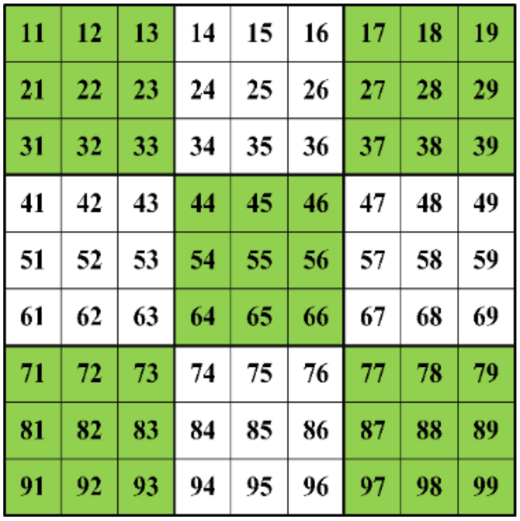
2.3. Configuration and Reconfiguration Techniques
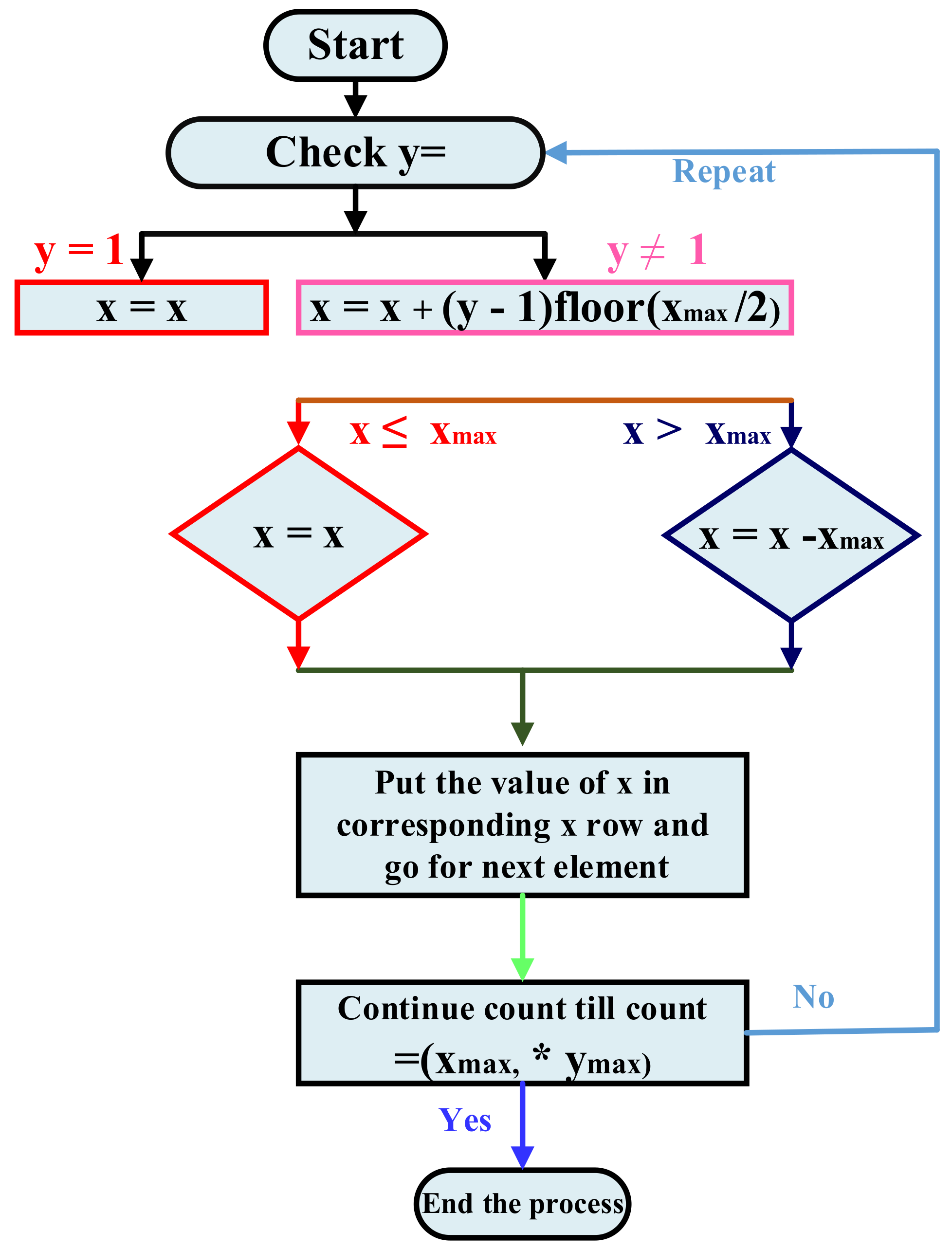
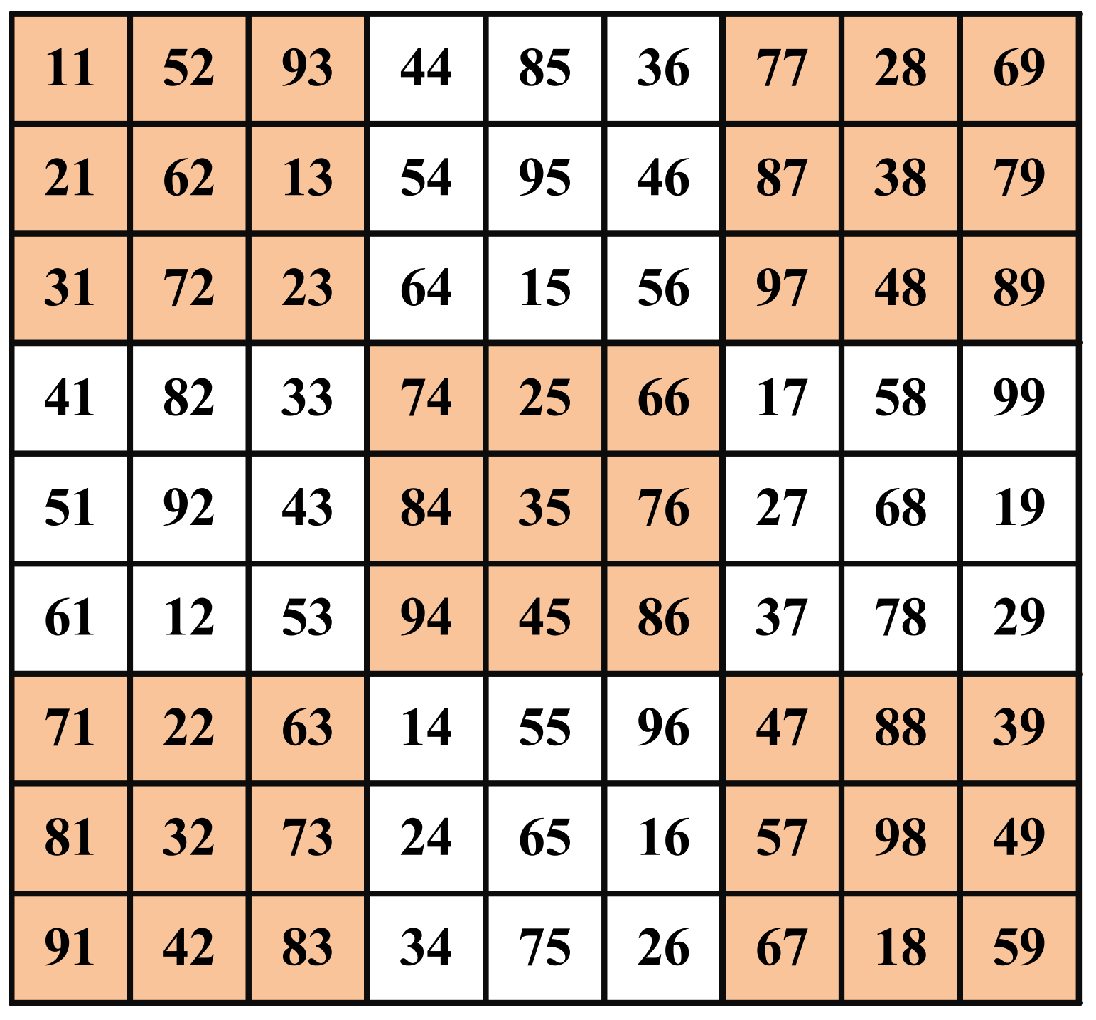
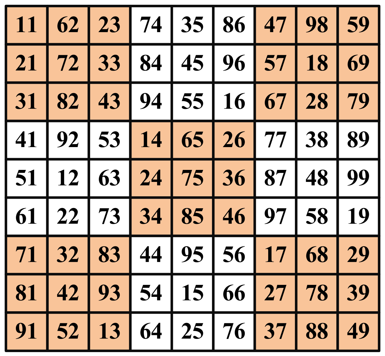
3. Non-Symmetrical (NS) Reconfiguration Technique
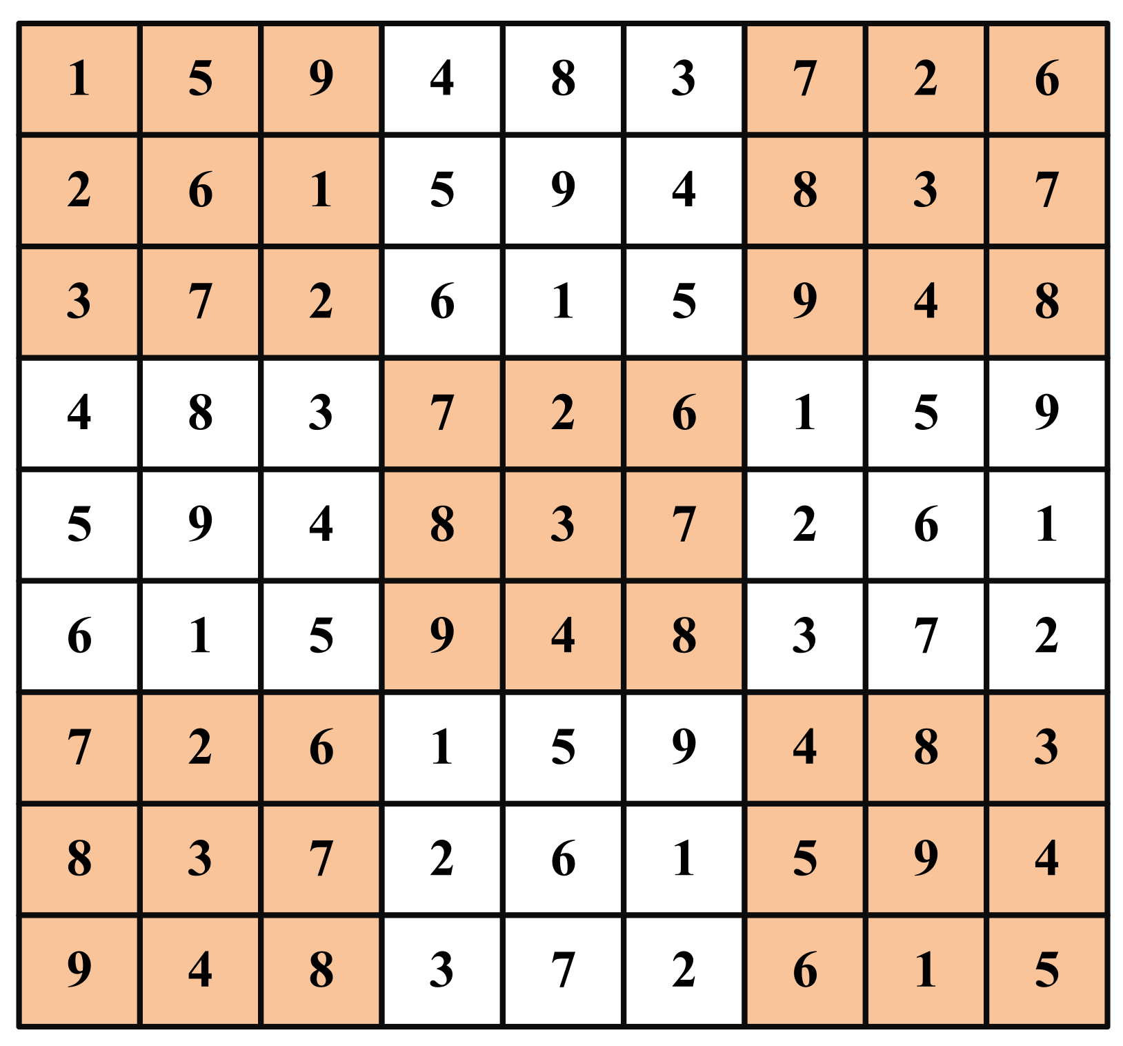
3.1. Algorithm/Rule for Non-Symmetrical Arrangement-1
| Algorithm 1. Algorithm for Non-Symmetrical Arrangement-1. |
if else |
3.2. Algorithm/Rule for Non-Symmetrical Arrangement-2
| Algorithm 2. Algorithm for Non-Symmetrical Arrangement-2. |
if else |
- It increases the power generated, FF, and efficiency.
- Power loss due to shading gets reduced as compared to the TCT configuration.
- It does not require any switching matrix such as the dynamic reconfiguration technique and relative losses.
- It reduces the local multiple power peaks in the PV curve and smoothens the PV curve.
- Additional cable power loss due to cable and requirement of a skilled person.
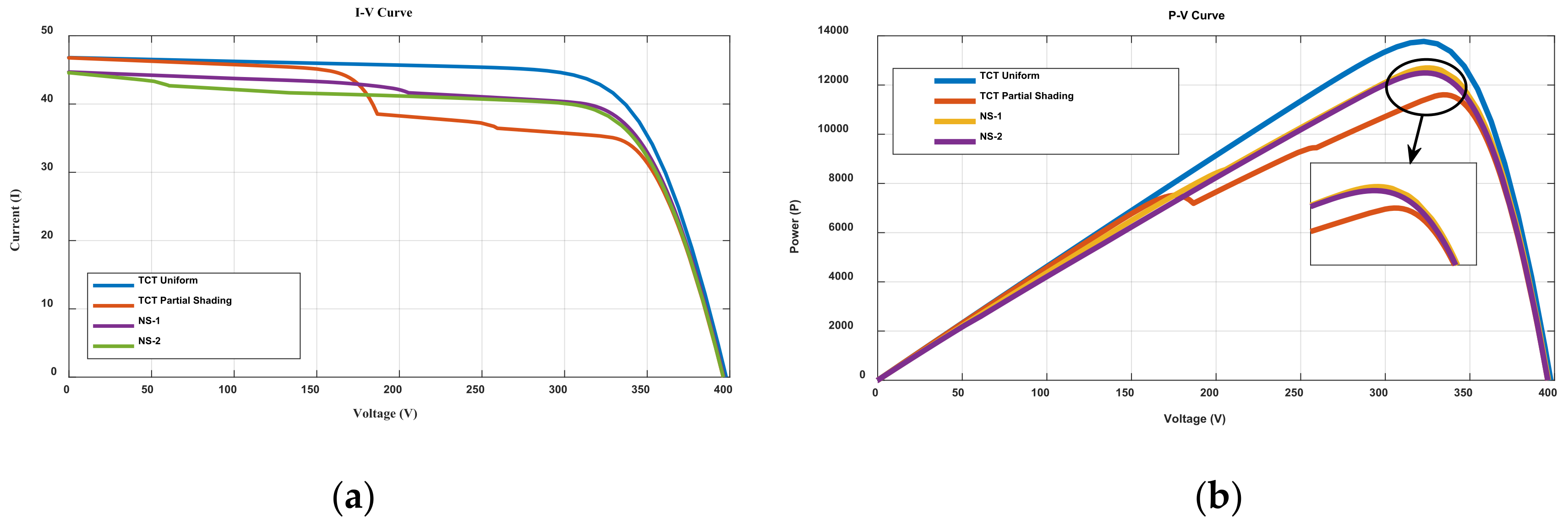
4. Results and Discussion
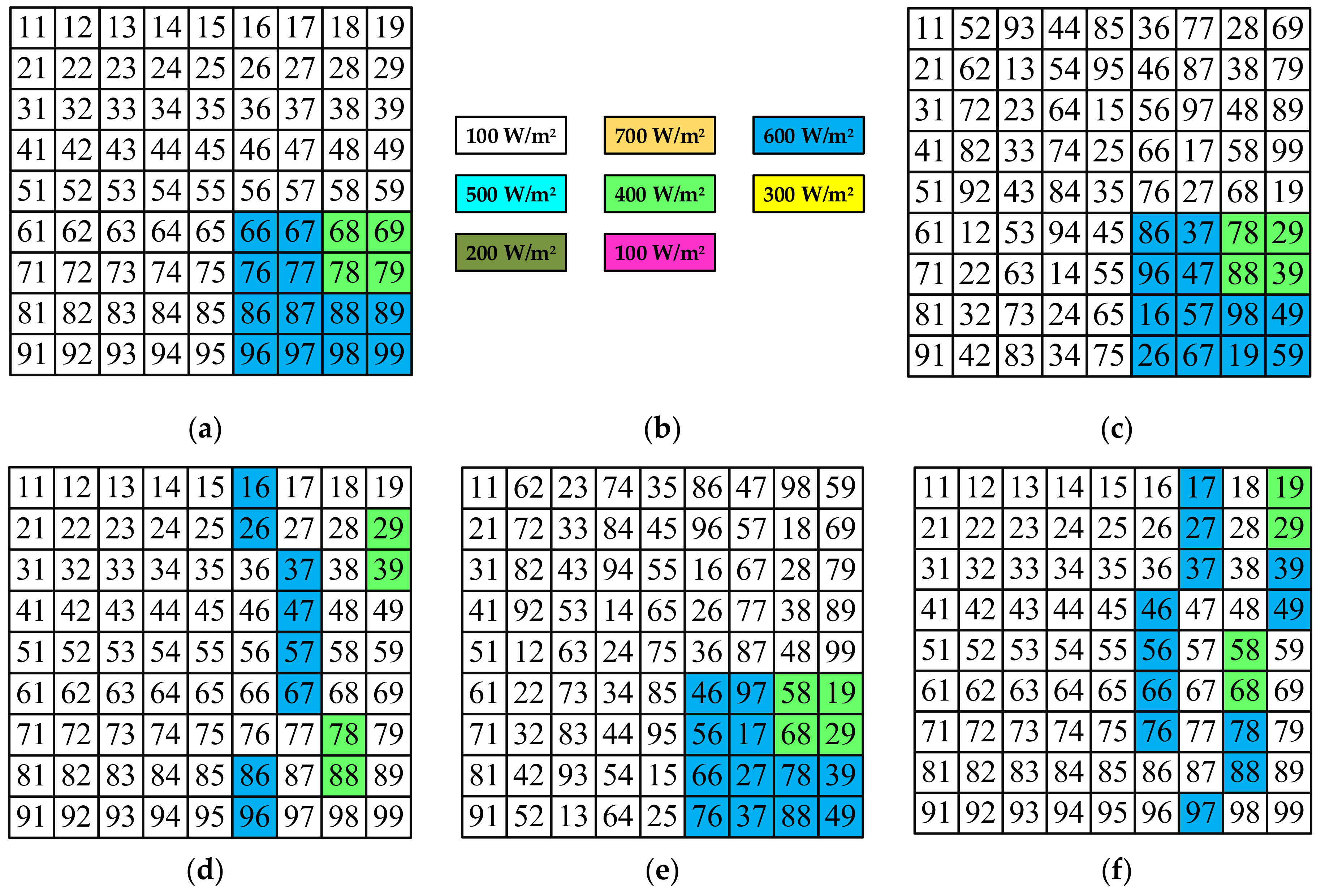
4.1. Normal Shading Condition
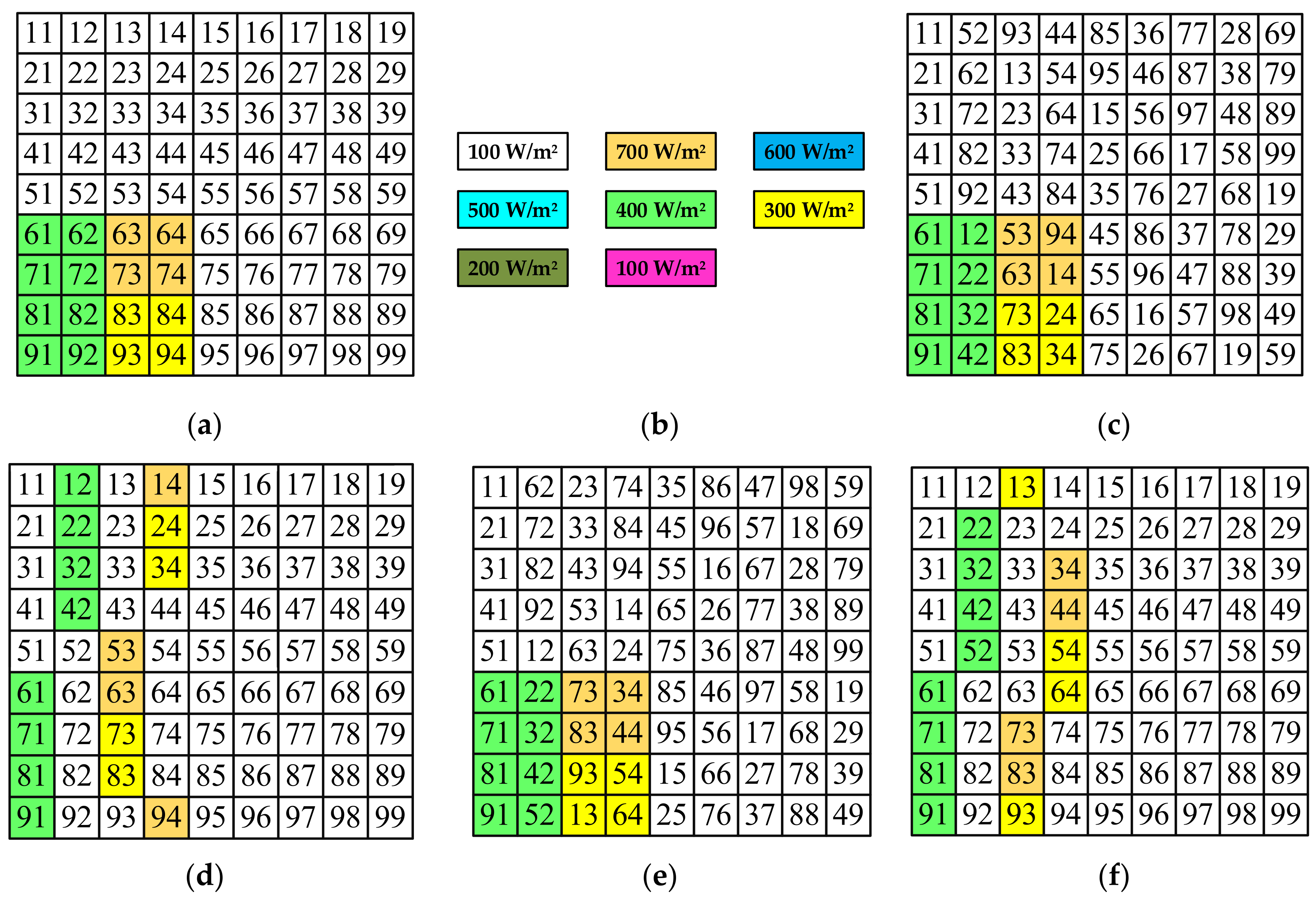
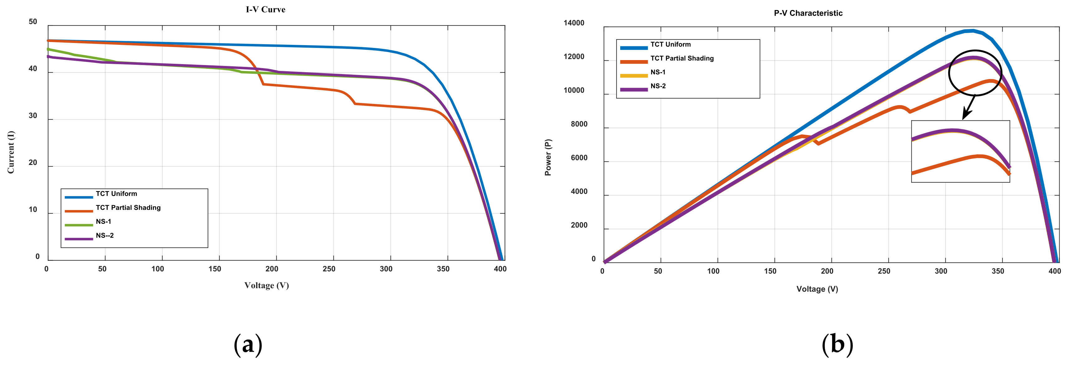
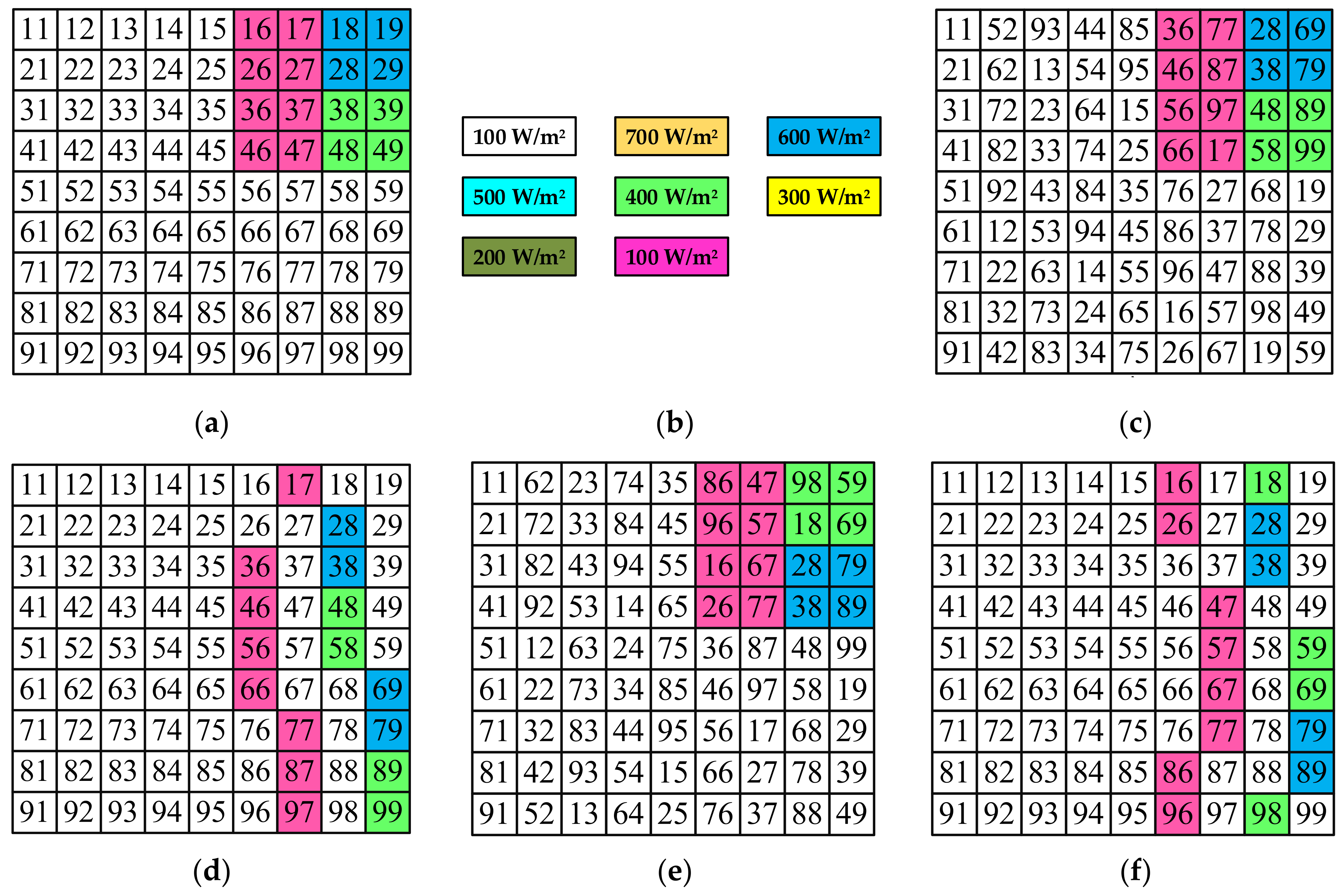
4.2. First: BORC 4 × 4 Sub-Array Shading Condition
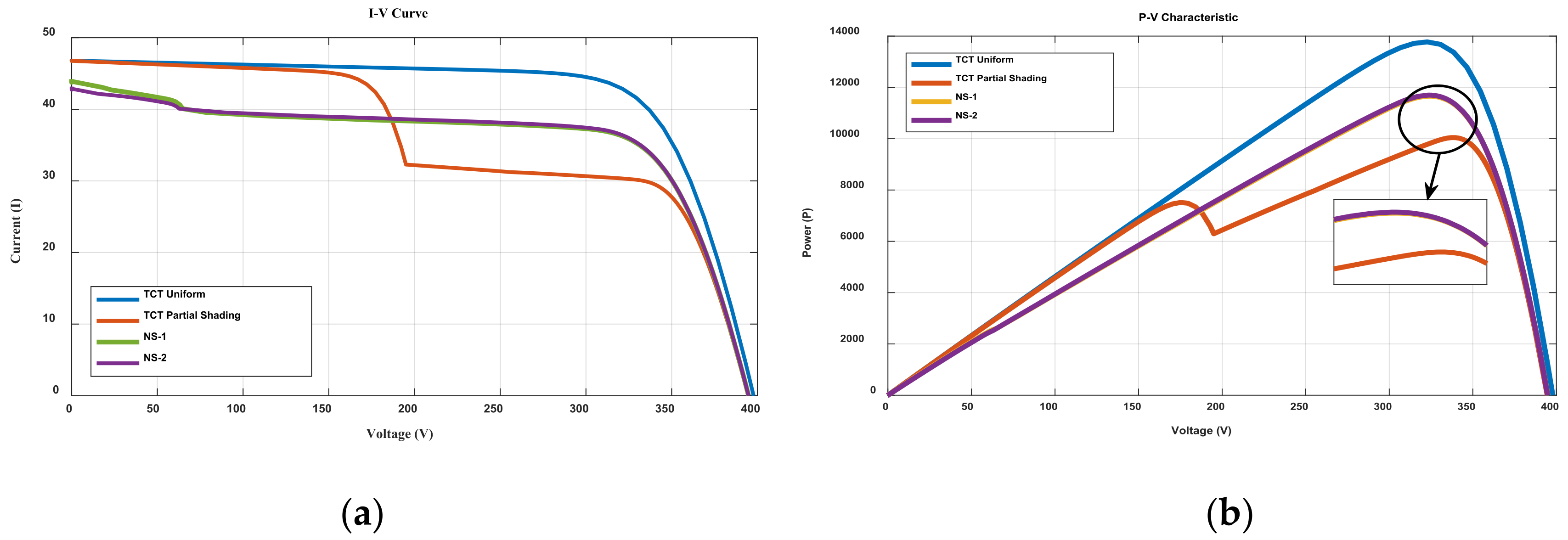
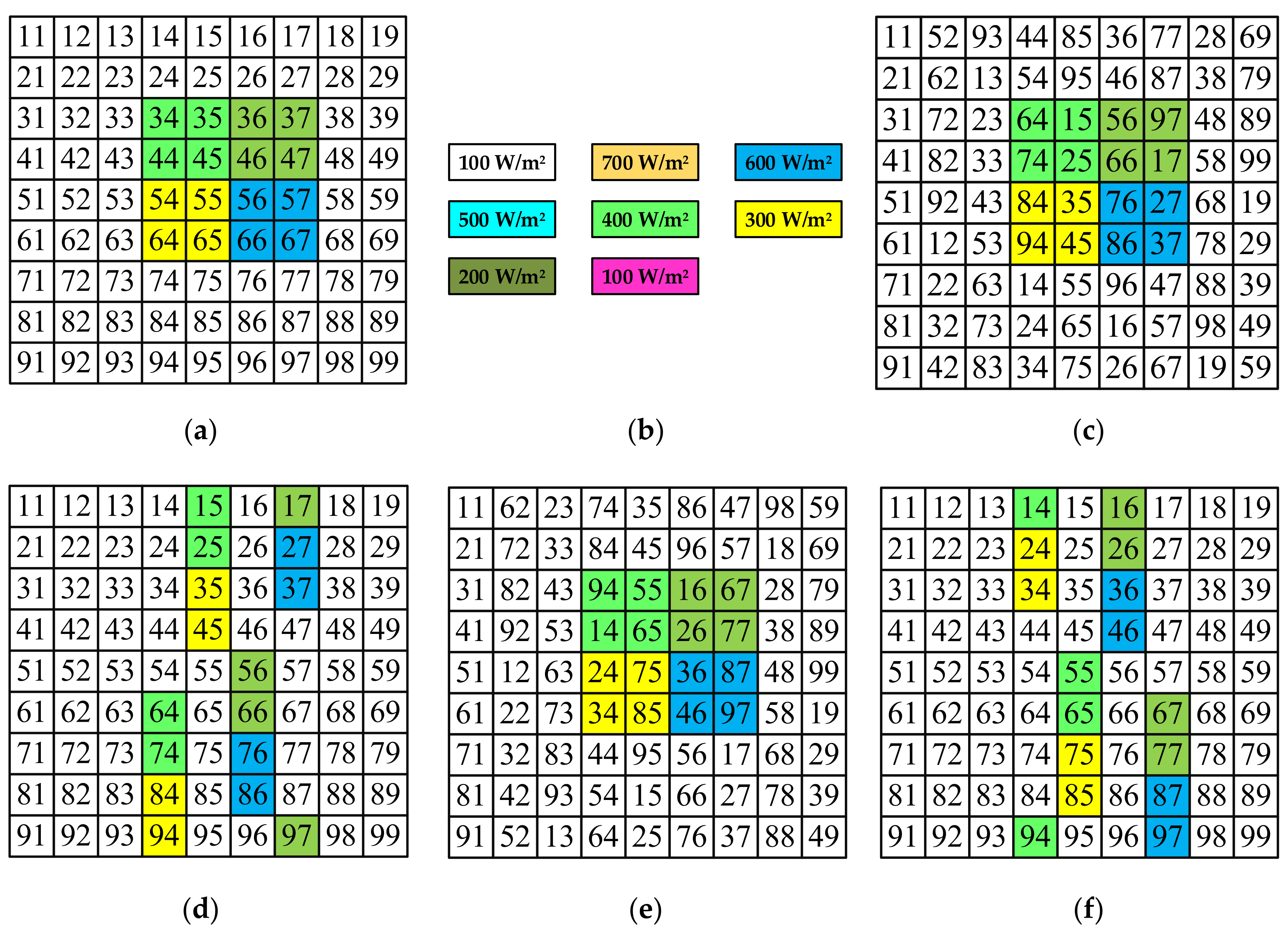
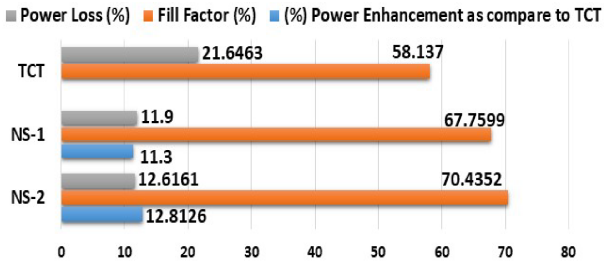
4.3. Second: BOLC 4 × 4 Sub-Array Shading Condition
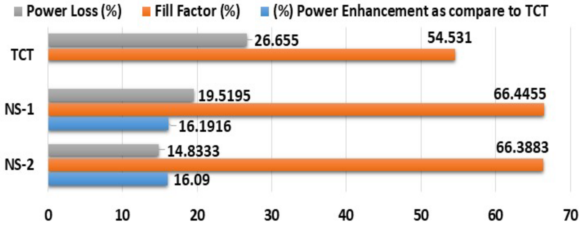
4.4. Third: TORC 4 × 4 Sub-Array Shading Condition
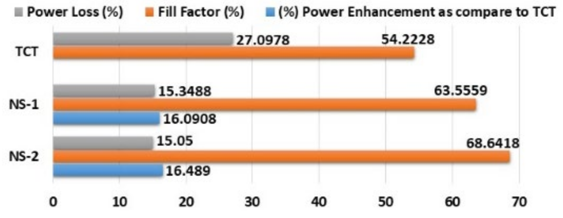
4.5. Fourth: TOLC 4 × 4 Sub-Array Shading Condition
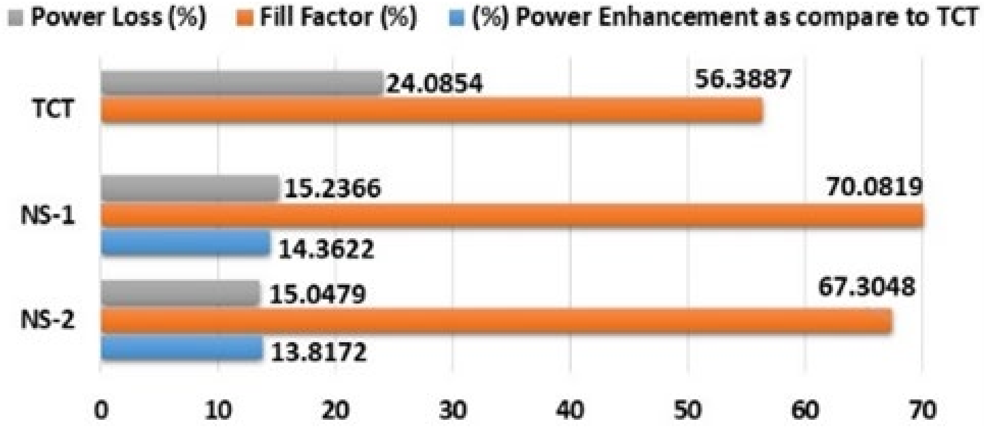
4.6. Fifth: 4 × 4 Sub-Array Shading Condition at Center
4.7. Sixth: Two Sub-Arrays of 3 × 3 Shading Condition
5. Conclusions
6. PV Module Used
Author Contributions
Funding
Institutional Review Board Statement
Informed Consent Statement
Data Availability Statement
Conflicts of Interest
References
- Hachim, B.; Dahlioui, D.; Barhdadi, A. Electrification of rural and arid areas by solar energy applications case study: Boumhaout village in south of Morocco. In Proceedings of the 2018 6th International Renewable and Sustainable Energy Conference, IRSEC 2018, Rabat, Morocco, 5–8 December 2018; Volume 1, pp. 1–4. [Google Scholar] [CrossRef]
- Choudhary, S. Global Energy Demand to Increase by 4.6% in 2021. 2020, pp. 11–12. Available online: https://economictimes.indiatimes.com/industry/energy/oil-gas/global-energy-demand-to-increase-by-4-6-in-2021-iea/articleshow/82163196.cms (accessed on 8 December 2021).
- Radhakrishnan, V. October Saw Highest Power Shortage in over 5 Years. 2021. Available online: https://www.thehindu.com/news/national/october-2021-saw-highest-power-shortage-in-over-5-years/article37361732.ece#:~:text=In%20October%2C%20Gujarat%20recorded%20a,in%20more%20than%20a%20decade (accessed on 28 November 2021).
- Negi, A.; Kumar, A. Long-term Electricity Demand Scenarios for India: Implications of Energy Efficiency. In Proceedings of the 2018 International Conference on Power Energy, Environment and Intelligent Control, PEEIC 2018, Greater Noida, India, 13–14 April 2018; pp. 462–467. [Google Scholar] [CrossRef]
- Meral, M.E.; Diner, F. A review of the factors affecting operation and efficiency of photovoltaic based electricity generation systems. Renew. Sustain. Energy Rev. 2011, 15, 2176–2184. [Google Scholar] [CrossRef]
- Jordehi, A.R. Maximum power point tracking in photovoltaic (PV) systems: A review of different approaches. Renew. Sustain. Energy Rev. 2016, 65, 1127–1138. [Google Scholar] [CrossRef]
- Chandrakant, C.V.; Mikkili, S. A typical review on static reconfiguration strategies in photovoltaic array under non-uniform shading conditions. CSEE J. Power Energy Syst. 2020, 1–33. [Google Scholar] [CrossRef]
- Boddapati, V.; Sree, A.; Nandikatti, R. Energy for Sustainable Development Salient features of the national power grid and its management during an emergency: A case study in India. Energy Sustain. Dev. 2020, 59, 170–179. [Google Scholar] [CrossRef]
- Kumar, N.; Tripathi, M.M. Solar Power Trading Models for Restructured Electricity Market in India. Asian J. Water Environ. Pollut. 2020, 17, 49–54. [Google Scholar] [CrossRef]
- Purohit, I.; Purohit, P. Performance assessment of grid-interactive solar photovoltaic projects under India’ s national solar mission. Appl. Energy 2018, 222, 25–41. [Google Scholar] [CrossRef] [Green Version]
- Wang, Y.; Das, R.; Putrus, G.; Kotter, R. Economic evaluation of photovoltaic and energy storage technologies for future domestic energy systems—A case study of the UK. Energy 2020, 203, 117826. [Google Scholar] [CrossRef]
- Christabel, S.C.; Srinivasan, A.; Winston, D.P.; Kumar, B.P. Reconfiguration solution for extracting maximum power in the aged solar PV systems. J. Electr. Eng. 2016, 16, 440–446. [Google Scholar]
- Braun, H.; Buddha, S.T.; Krishnan, V.; Tepedelenlioglu, C.; Spanias, A.; Banavar, M.; Srinivasan, D. Topology reconfiguration for optimization of photovoltaic array output. Sustain. Energy Grids Netw. 2016, 6, 58–69. [Google Scholar] [CrossRef] [Green Version]
- Agarwal, N.; Agarwal, A. Mismatch Losses in Solar Photovoltaic Array. MIT Int. J. Electr. Instrum. Eng. 2014, 4, 16–19. [Google Scholar]
- Horoufiany, M.; Ghandehari, R. Optimal fixed reconfiguration scheme for PV arrays power enhancement under mutual shading conditions. IET Renew. Power Gener. 2017, 11, 1456–1463. [Google Scholar] [CrossRef]
- Postovoit, B.; Susoeff, D.; Daghbas, D.; Holt, J.; Pomona, C.P.; Le, H.T. A Solar-Based Stand-Alone Family House for Energy Independence and Efficiency. In Proceedings of the 2020 IEEE Conference on Technologies for Sustainability, SusTech 2020, Santa Ana, CA, USA, 23–25 April 2020. [Google Scholar] [CrossRef]
- Chavan, V.C.; Mikkili, S. Effect of PV Array Positioning on Mismatch and Wiring Losses in Static Array Reconfiguration. IETE J. Res. 2021, 1–14. [Google Scholar] [CrossRef]
- Pendem, S.R.; Mikkili, S. Modeling, simulation, and performance analysis of PV array configurations (Series, Series-Parallel, Bridge-Linked, and Honey-Comb) to harvest maximum power under various Partial Shading Conditions. Int. J. Green Energy 2018, 15, 795–812. [Google Scholar] [CrossRef]
- Manjunath Suresh, H.N.; Rajanna, S. Performance enhancement of Hybrid interconnected Solar Photovoltaic array using shade dispersion Magic Square Puzzle Pattern technique under partial shading conditions. Sol. Energy 2019, 194, 602–617. [Google Scholar] [CrossRef]
- Kumar, B.P.; Cherukuri, S.K.; Kaniganti, K.R.; Karuppiah, N.; Muniraj, R. Performance Enhancement of Partial Shaded Photovoltaic System With the Novel Screw Pattern Array Configuration Scheme. IEEE Access 2022, 10, 1731–1744. [Google Scholar] [CrossRef]
- Bonthagorla, P.K.; Mikkili, S. A Novel Fixed PV Array Configuration for Harvesting Maximum Power from Shaded Modules by Reducing the Number of Cross-Ties. IEEE J. Emerg. Sel. Top. Power Electron. 2020, 9, 2109–2121. [Google Scholar] [CrossRef]
- Ajmal, A.M.; Sudhakar Babu, T.; Ramachandaramurthy, V.K.; Yousri, D.; Ekanayake, J.B. Static and dynamic reconfiguration approaches for mitigation of partial shading influence in photovoltaic arrays. Sustain. Energy Technol. Assess. 2020, 40, 100738. [Google Scholar] [CrossRef]
- Pachauri, R.K.; Alhelou, H.H.; Bai, J.; Golshan, M.E.H. Adaptive Switch Matrix for PV Module Connections to Avoid Permanent Cross-Tied Link in PV Array System under Non-Uniform Irradiations. IEEE Access 2021, 9, 45978–45992. [Google Scholar] [CrossRef]
- Ngo, T.; Nguyen, Q.; Nguyen, L.; Riva, E.; Romano, P.; Viola, F. Increasing efficiency of photovoltaic systems under non-homogeneous solar irradiation using improved Dynamic Programming methods. Sol. Energy 2017, 150, 325–334. [Google Scholar] [CrossRef]
- Srinivasan, A.; Devakirubakaran, S. L-Shape Propagated Array Configuration With Dynamic Reconfiguration Algorithm for Enhancing Energy Conversion Rate of Partial Shaded Photovoltaic Systems. IEEE Access 2021, 9, 97661–97674. [Google Scholar] [CrossRef]
- Malathy, S.; Ramaprabha, R. Reconfiguration strategies to extract maximum power from photovoltaic array under partially shaded conditions. Renew. Sustain. Energy Rev. 2018, 81, 2922–2934. [Google Scholar] [CrossRef]
- Chavan, V.C.; Mikkili, S. Repositioning of Series-Parallel, Total-Cross-Tide, Bridge-Link, and Honey-Comb PV Array Configurations for Maximum Power Extraction. IETE J. Res. 2021, 1–13. [Google Scholar] [CrossRef]
- Rani, B.I.; Ilango, G.S.; Nagamani, C. Enhanced power generation from PV array under partial shading conditions by shade dispersion using Su Do Ku configuration. IEEE Trans. Sustain. Energy 2013, 4, 594–601. [Google Scholar] [CrossRef]
- Sai Krishna, G.; Moger, T. Improved SuDoKu reconfiguration technique for total-cross-tied PV array to enhance maximum power under partial shading conditions. Renew. Sustain. Energy Rev. 2019, 109, 333–348. [Google Scholar] [CrossRef]
- El Iysaouy, L.; Lahbabi, M.; Oumnad, A. A novel magic square view topology of a PV system under partial shading condition. Energy Procedia 2019, 157, 1182–1190. [Google Scholar] [CrossRef]
- Sreekantha Reddy, S.; Yammani, C. A novel Magic-Square puzzle based one-time PV reconfiguration technique to mitigate mismatch power loss under various partial shading conditions. Optik 2020, 222, 165289. [Google Scholar] [CrossRef]
- Nihanth, M.S.S.; Ram, J.P.; Pillai, D.S.; Ghias, A.M.; Garg, A.; Rajasekar, N. Enhanced power production in PV arrays using a new skyscraper puzzle based one-time reconfiguration procedure under partial shade conditions (PSCs). Sol. Energy 2019, 194, 209–224. [Google Scholar] [CrossRef]
- Pillai, D.S.; Rajasekar, N.; Ram, J.P.; Chinnaiyan, V.K. Design and testing of two phase array reconfiguration procedure for maximizing power in solar PV systems under partial shade conditions (PSC). Energy Convers. Manag. 2018, 178, 92–110. [Google Scholar] [CrossRef]


| 3 | 2 | 1 |
| 5 | 3 | 2 |
| 7 | 4 | 3 |
| 9 | 5 | 4 |
| Column 1 | Column 2 = | Column 3 = | Column 4 = | Column 5 = | Column 6 = | Column 7 = | Column 8 = | Column 9 = |
|---|---|---|---|---|---|---|---|---|
| Column 1 | Column 1 + 4 | Column 2 + 4 | Column 3 + 4 | Column 4 + 4 | Column 5 + 4 | Column 6 + 4 | Column 7 + 4 | Column 8 + 4 |
| 1 | 5 | 9 | 13 − 9 = 4 | 8 | 12 − 9 = 3 | 7 | 11 − 9 = 2 | 6 |
| 2 | 6 | 10 − 9 = 1 | 5 | 9 | 13 − 9 = 4 | 8 | 12 − 9 = 3 | 7 |
| 3 | 7 | 11 − 9 = 2 | 6 | 10 − 9 = 1 | 5 | 9 | 13 − 9 = 4 | 8 |
| 4 | 8 | 12 − 9 = 3 | 7 | 11 − 9 = 2 | 6 | 10 − 9 = 1 | 5 | 9 |
| 5 | 9 | 13 − 9 = 4 | 8 | 12 − 9 = 3 | 7 | 11-9 = 2 | 6 | 10 − 9 = 1 |
| 6 | 10 − 9 = 1 | 5 | 9 | 13 − 9 = 4 | 8 | 12 − 9 = 3 | 7 | 11 − 9 = 2 |
| 7 | 11 − 9 = 2 | 6 | 10 − 9 = 1 | 5 | 9 | 13 − 9 = 4 | 8 | 12 − 9 = 3 |
| 8 | 12 − 9 = 3 | 7 | 11 − 9 = 2 | 6 | 10 − 9 = 1 | 5 | 9 | 13 − 9 = 4 |
| 9 | 13 − 9 = 4 | 8 | 12 − 9 = 3 | 7 | 11 − 9 = 2 | 6 | 10 − 9 = 1 | 5 |
| Column 1 | Column 2 = | Column 3 = | Column 4 = | Column 5 = | Column 6 = | Column 7 = | Column 8 = | Column 9 = |
|---|---|---|---|---|---|---|---|---|
| Column 1 | Column 1 + 4 | Column 2 + 4 | Column 3 + 4 | Column 4 + 4 | Column 5 + 4 | Column 6 + 4 | Column 7 + 4 | Column 8 + 4 |
| 1 | 6 | 11 − 9 = 2 | 7 | 12 − 9 = 3 | 8 | 13 − 9 = 4 | 9 | 14 − 9 = 5 |
| 2 | 7 | 12 − 9 = 3 | 8 | 13 − 9 = 4 | 9 | 14 − 9 = 5 | 10 − 9 = 1 | 6 |
| 3 | 8 | 13 − 9 = 4 | 9 | 14 − 9 = 5 | 10 − 9 = 1 | 6 | 11 − 9 = 2 | 7 |
| 4 | 9 | 14 − 9 = 5 | 10 − 9 = 1 | 6 | 11 − 9 = 2 | 7 | 12 − 9 = 3 | 8 |
| 5 | 10 − 9 = 1 | 15 − 9 = 6 | 11 − 9 = 2 | 7 | 12 − 9 = 3 | 8 | 13 − 9 = 4 | 9 |
| 6 | 11 − 9 = 2 | 7 | 12 − 9 = 3 | 8 | 13 − 9 = 4 | 9 | 14 − 9 = 5 | 10 − 9 = 1 |
| 7 | 12 − 9 = 3 | 8 | 13 − 9 = 4 | 9 | 14 − 9 = 5 | 10 − 9 = 1 | 6 | 11 − 9 = 2 |
| 8 | 13 − 9 = 4 | 9 | 14 − 9 = 5 | 10 − 9 = 1 | 6 | 11 − 9 = 2 | 7 | 12 − 9 = 3 |
| 9 | 14 − 9 = 5 | 10 − 9 = 1 | 6 | 11 − 9 = 2 | 7 | 12 − 9 = 3 | 8 | 13 − 9 = 4 |
| GMPP (Watt) | ||||
|---|---|---|---|---|
| 397.8 | 46.9539 | 13,773 | 321.4876 | 42.8414 |
| Method | GMPP (Watt) | % Power Loss | % Fill Factor | ||||
|---|---|---|---|---|---|---|---|
| TCT | 396.0500 | 46.9407 | 11,605 | 34.8333 | 335.3143 | 15.7409 | 62.4231 |
| NS1 | 396.4674 | 44.8539 | 12,696 | 38.9835 | 325.6884 | 7.8196 | 71.3935 |
| NS2 | 396.075 | 44.8096 | 12,486 | 38.3018 | 325.9793 | 9.3443 | 70.3517 |
| Method | Voc (Volts) | Isc (Ampere) | GMPP (Watt) | IGMPP (Ampere) | VGMPP (Volts) | % Power Loss | % Fill Factor |
|---|---|---|---|---|---|---|---|
| TCT | 395.5285 | 46.9407 | 10,794 | 31.6932 | 340.5731 | 21.6463 | 58.1370 |
| NS1 | 395.6759 | 45.2576 | 12,134 | 37.5343 | 323.2727 | 11.9000 | 67.7599 |
| NS2 | 395.6798 | 43.6925 | 12,177 | 37.4041 | 325.5426 | 11.5800 | 70.4352 |
| Method | Voc (Volts) | Isc (Ampere) | GMPP (Watt) | IGMPP (Ampere) | VGMPP (Volts) | % Power Loss | % Fill Factor |
|---|---|---|---|---|---|---|---|
| TCT | 394.7300 | 46.9407 | 10,104 | 29.6743 | 340.4987 | 26.6550 | 54.5310 |
| NS1 | 394.9547 | 44.7358 | 11,740 | 36.2547 | 323.8321 | 14.7600 | 66.4455 |
| NS2 | 394.9578 | 44.7358 | 11,730 | 35.8959 | 326.7896 | 14.8333 | 66.3883 |
| Method | Voc (Volts) | Isc (Ampere) | GMPP (Watt) | IGMPP (Ampere) | VGMPP (Volts) | % Power Loss | % Fill Factor |
|---|---|---|---|---|---|---|---|
| TCT | 394.5770 | 46.9407 | 10,043 | 29.7798 | 337.2400 | 27.0978 | 54.2228 |
| NS1 | 394.7959 | 44.2141 | 11,659 | 35.9232 | 325.1889 | 15.3488 | 66.7925 |
| NS2 | 394.7943 | 43.1707 | 11,699 | 36.0765 | 324.2842 | 15.0500 | 68.6418 |
| Voc (Volts) | Isc (Ampere) | GMPP (Watt) | IGMPP (Ampere) | VGMPP (Volts) | % Power Loss | % Fill Factor |
|---|---|---|---|---|---|---|
| 395.1000 | 46.9407 | 10,458 | 30.7980 | 339.5553 | 24.0854 | 56.3887 |
| 395.3085 | 43.1707 | 11,960 | 36.8704 | 324.3865 | 13.1634 | 70.0819 |
| 395.3257 | 44.7358 | 11,903 | 36.6855 | 324.4683 | 13.5772 | 67.3048 |
| Method | Voc (Volts) | Isc (Ampere) | GMPP (Watt) | IGMPP (Ampere) | VGMPP (Volts) | % Power Loss | % Fill Factor |
|---|---|---|---|---|---|---|---|
| TCT | 395.0000 | 46.9210 | 10,892 | 32.5142 | 335.0006 | 20.9349 | 58.7683 |
| NS1 | 395.1058 | 44.7358 | 11,546 | 34.8785 | 331.0442 | 16.1693 | 65.3225 |
| NS2 | 395.0062 | 44.7358 | 11,545 | 34.9012 | 330.8230 | 16.1765 | 65.3333 |
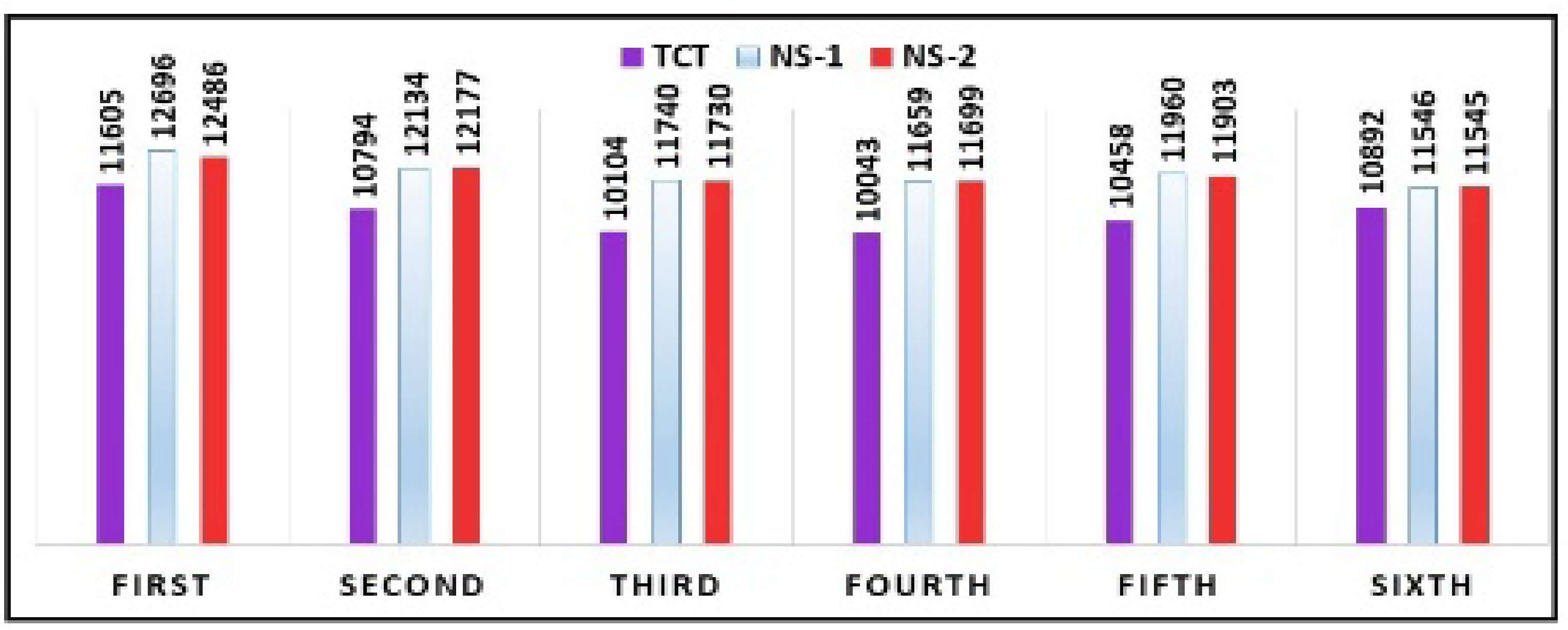
| Sixth | 10,892 | 11,546 | 11,545 | 06.0044 | 5.99520 | ||
| Shading Type | % Power Enhanced in NS-1 Compared to TCT | % Power Enhanced in NS-2 Compared to TCT | ||||
|---|---|---|---|---|---|---|
| First | 11,605 | 12,696 | 12,486 | 09.4011 | 07.5900 | |
| Second | 10,794 | 12,134 | 12,177 | 12.4143 | 12.8126 | |
| Third | 10,104 | 11,740 | 11,730 | 16.1916 | 16.0900 | |
| Fourth | 10,043 | 11,659 | 11,699 | 16.0908 | 16.4890 | |
| Fifth | 10,458 | 11,960 | 11,903 | 14.3622 | 13.8172 | |
| Parameter | Ratings |
|---|---|
| Power | 170 W |
| 44.2 V | |
| 5.2 A | |
| 35.8 V | |
| 4.75 A | |
| Number of cells | 72 |
Publisher’s Note: MDPI stays neutral with regard to jurisdictional claims in published maps and institutional affiliations. |
© 2022 by the authors. Licensee MDPI, Basel, Switzerland. This article is an open access article distributed under the terms and conditions of the Creative Commons Attribution (CC BY) license (https://creativecommons.org/licenses/by/4.0/).
Share and Cite
Mikkili, S.; Kanjune, A.; Bonthagorla, P.K.; Senjyu, T. Non-Symmetrical (NS) Reconfiguration Techniques to Enhance Power Generation Capability of Solar PV System. Energies 2022, 15, 2124. https://doi.org/10.3390/en15062124
Mikkili S, Kanjune A, Bonthagorla PK, Senjyu T. Non-Symmetrical (NS) Reconfiguration Techniques to Enhance Power Generation Capability of Solar PV System. Energies. 2022; 15(6):2124. https://doi.org/10.3390/en15062124
Chicago/Turabian StyleMikkili, Suresh, Akshay Kanjune, Praveen Kumar Bonthagorla, and Tomonobu Senjyu. 2022. "Non-Symmetrical (NS) Reconfiguration Techniques to Enhance Power Generation Capability of Solar PV System" Energies 15, no. 6: 2124. https://doi.org/10.3390/en15062124
APA StyleMikkili, S., Kanjune, A., Bonthagorla, P. K., & Senjyu, T. (2022). Non-Symmetrical (NS) Reconfiguration Techniques to Enhance Power Generation Capability of Solar PV System. Energies, 15(6), 2124. https://doi.org/10.3390/en15062124