Experimental Analysis of Flow Boiling in Horizontal Annulus—The Effect of Heat Flux on Bubble Size Distributions ^†

Abstract

Subcooled flow boiling was experimentally investigated in a horizontal annulus with a temperature-controlled boiling surface and transparent outer pipe facilitating visualization. Boiling occurs on a copper tube with a diameter of 12 mm in an annulus with a 2 mm gap. Refrigerant R245fa is used as a working fluid. The focus of this study is to explore the effect of heat flux variation on the boiling flow patterns at approximately constant inlet flow conditions of the working fluid (fixed mass flux and inlet fluid temperature). Subcooled flow boiling is recorded by a high-speed camera, images are analyzed by a neural network to determine the bubble size distributions and their variation with the heat flux. The experimental setup being a part of the laboratory THELMA (Thermal Hydraulics experimental Laboratory for Multiphase Applications) at the Reactor Engineering Division of Jožef Stefan Institute, analysis methods and measurement results are presented and discussed.

1. Introduction

Flow boiling is a heat transfer mechanism allowing high surface heat flux at low temperature differences. As such, it is used in many systems, from air conditioners [1], power electronics cooling [2] and large power systems such as thermal power plants and nuclear reactors [3]. Despite its wide use and long history of research, accurate predictions still rely on many experimentally based correlations, developed for specific fluids, geometries, flow orientations, surface types, pressures, etc. Similarly, accurate numerical simulations of general two-phase flows are computationally very expensive and despite the progress in computational power, they still require some modeling by constitutional relations. For a better understanding of the underlying phenomena, the development of new models and for validation of simulations, experimental data are of crucial importance. Besides heat transfer and pressure drop predictions, bubble size, bubble departure frequency, vapor (i.e., void fraction) distribution are also important quantities to consider.

Traditionally, bubble diameters and void fractions were reported as integral or time-averaged values at certain locations [4,5,6], with little or no information on the distribution of bubble sizes. Several authors report the departure, maximum and characteristic bubble sizes, both from experimental [7,8,9] and numerical points of view [10,11].

With the advancement of high-speed imaging techniques and analysis methods with a concurrent increase in computational power, the interest for detailed analysis of these quantities has increased.

Golobič and Zupančič [12,13] measured local wall-temperature and heat flux distributions by fast IR thermography in pool boiling of water. Similar measurements were recently performed in flow boiling in semi-annular geometry by Scheiff et al. [14]. They observed flow boiling through the outer glass tube with a high-speed camera and measured IR bubble footprints on the boiling surface made of thin electrically-heated metal foil. Among other results, they reported that bubble diameters follow a normal distribution.

Although several authors have measured and described bubble size distributions in narrow tubes and channels, only a few papers describe these data in annular geometries. Zeitoun et al. [15] investigated bubble behavior in subcooled boiling of water in a vertical annulus with an inner tube diameter of 12.7 mm and 6.3 mm gap size. They used high-speed imaging and image processing to determine the mean bubble diameter after departure. Lee et al. [16] measured radial profiles of local void fractions in a vertical annulus in subcooled boiling of water with a 19 mm inner tube and 9.3 mm gap size. Two point-conductivity probes were used for local void fraction measurements.

To the authors’ knowledge, the paper by Ugandhar et al. [17] is the only one reporting experimental results of the distribution of bubble sizes in a horizontal annulus. They have studied the effect of pressure on bubble size distribution in a horizontal annulus (6.5 mm gap) with boiling water as a working fluid. A high-speed camera was used and automated image processing was performed. All mentioned experiments used electric resistance heating (heat flux control) of the boiling surface.

In this paper, bubble distributions in a horizontal annulus with a 12.5 mm water-heated internal tube and a 2 mm gap are measured. Refrigerant R245fa (pentafluoropropane) is used as a working fluid and a high-speed camera with semi-automatic neural network image processing is used to determine the bubble size distributions and their change with the heat flux. This is the first attempt to measure the bubble size distributions in temperature-controlled boiling within a horizontal annulus.

2. Experimental Setup

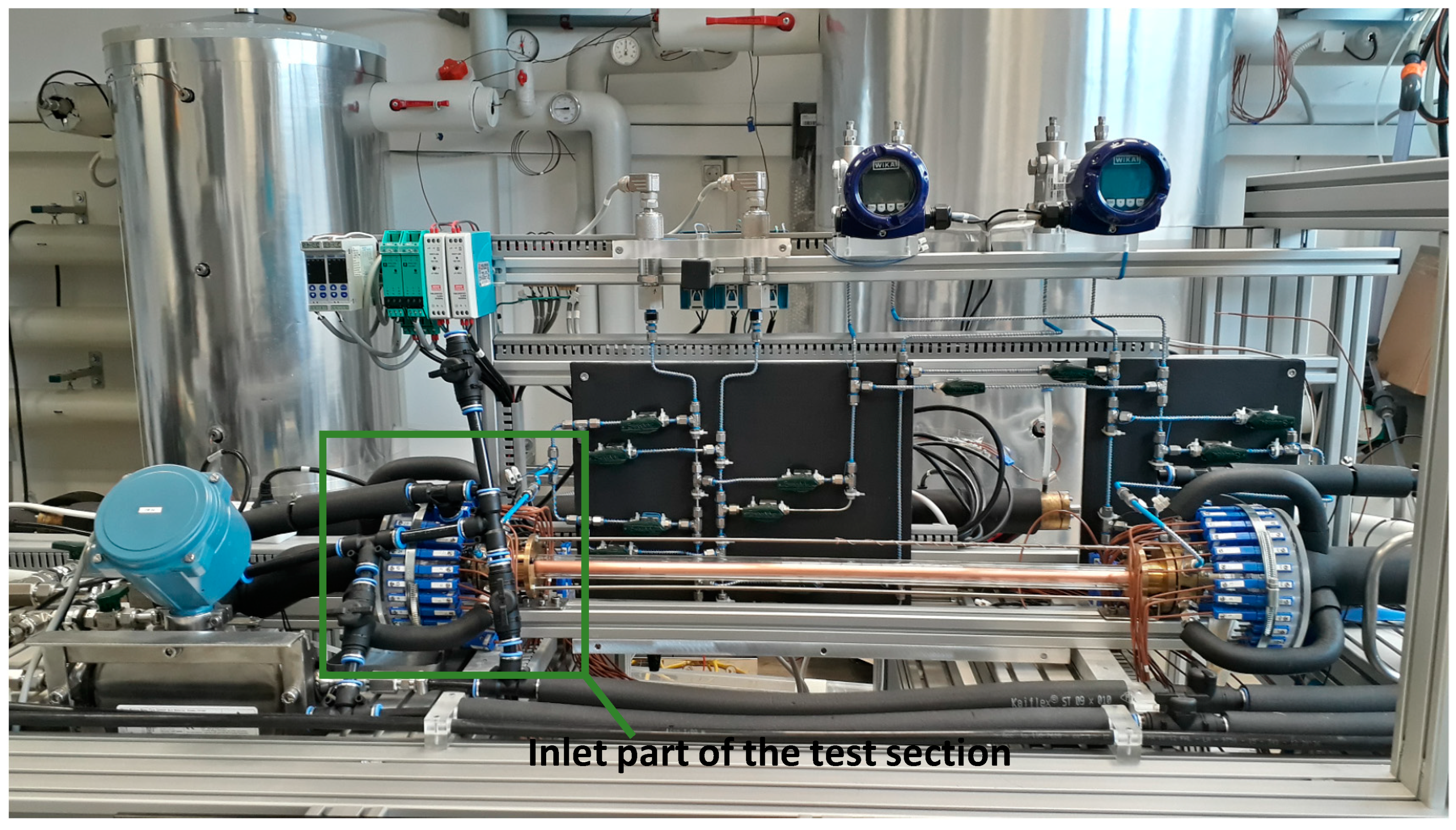
The main part of the experimental setup (Figure 1) is a water-heated horizontal annular test section, thoroughly described in our previous works [18,19,20]. Boiling occurs on the outer surface of the inner copper tube with a diameter of 12 mm and a total heated length of 585 mm. The annular gap between the copper tube and the outer glass tube is 2 mm. The outer surface of the copper tube is polished with sandpaper grit 400 to provide a uniform distribution of the nucleation sites. Boiling is observed with a high-speed camera through a borosilicate glass tube.

The test section is designed as a concentric tube heat exchanger (Figure 2), which allows a temperature-controlled flow boiling. Hot water flowing inside the copper tube transfers heat to the refrigerant flow (R245fa) in the annulus, which starts to boil on the outer surface of the copper tube at relatively low temperatures (30 °C at 1.8 bar) [21]. The finned structure inside the copper tube provides strong heat transfer enhancement with a homogeneous radial distribution and allows local temperature measurements along the tube axis. As the wall heat flux depends on the temperature difference between the heating water and the boiling refrigerant, no thermal runaway is possible if the critical heat flux value is reached. Both co-current and counter-current operations are possible in the test section. We have used co-current operation (refrigerant and water flowing in the same direction) to achieve the maximum temperature difference between water and refrigerant in the inlet region.

Measurement equipment is listed in

Table 1. Measurement equipment and its nominal uncertainty.

Quantity	Instrument	Nominal Range	Uncertainty
Abs. pressure	WIKA P-30	1–6 bar	±0.1%
Pressure drop	WIKA DPT-10	1–300 mbar	±0.1%
Inlet temperature	T-type thermocouple	10–70 °C	±0.5 °C
Inlet/outlet ΔT	Two-junction thermopile	0–100 °C	<0.1 °C
Test section temperatures	T-type thermocouple	10–70 °C	±0.1 °C
Mass flow rate, water	Coriolis flow meter	0.01–300 kg/h	±0.5%
Mass flow rate, R245fa	Coriolis flow meter	0.01–300 kg/h	±0.5%

. Thermocouples in contact with the heating water, positioned 21 ± 0.5 mm apart, measure the local temperature of the water. Two thermocouples at the water and refrigerant inlets are used to measure the inlet temperature of the liquid and two additional two-junction thermopiles are used to measure temperature difference toward the outlet. Thermocouples inside the test section are primarily used for the calculation of surface heat flux in the test section and were therefore cross-calibrated in a steady-state temperature situation with only water flowing through the test section to lower systematic errors. All thermocouples on the test section are referenced to the Kaye-170e artificial triple point of water.

Two Micro Motion Emerson Coriolis flow meters are used for direct measurements of water and refrigerant mass flow rate. From these values, the mass flux (i.e., mass flow area density) can be determined based on the cross-section area of the annulus. For absolute pressure and pressure drop, WIKA membrane sensors are used (see Table 1).

National Instruments PXIe500 with LabVIEW software was used for temperature, pressure and mass flow rate data acquisition.

As shown in Figure 3, the test section is supplied with refrigerant through a closed loop. The refrigerant flows from the pump, through the Coriolis mass flow meter and preheater, to the test section where it boils and returns to the condenser. Two adjacent water loops provide heating and cooling water for the heat exchangers and heating of the test section. Temperature-controlled pressurizer, connected to the main refrigerant loop right after the pump, controls the overall system pressure. The pressurizer is a closed vessel containing a large water–refrigerant heat exchanger to control the saturation temperature in the system. The Lauda thermal bath controls the pressurizer temperature.

For the visualization of the flow, a separate system is used. Phantom v1212 12-bit grayscale high-speed camera is used with a 100 mm macro lens, enabling the observation area of approx. 3.6 × 1.6 cm on the test section. The high-speed camera is a part of the LaVision PIV system with a built-in frame grabber and triggering functions. To reduce shadows and reflections in the recording, an even and diffuse lighting has to be used. In addition, the camera aperture needs to be closed as much as possible to achieve a large depth of focus, requiring the use of high-power lighting. For this task, a U-shaped light (Figure 4) was constructed from LED strips. High-power 20 W/m daylight color LED strips with a luminosity of approx. 2500 lumen/m were used. With this setup, the test section is mostly uniformly illuminated, with the notable exception of the direction directly from the camera view (darker line present in the middle of flow patterns depicted in Figure 5).

3. Experimental Procedure

Experiments were performed at two instances of constant refrigerant inlet conditions and at different temperatures of the heating water, to study the effect of heating power and therefore the heat flux separately from other possible effects.

For all cases considered in this study (see

Table 2. Experimental cases. Uncertainties stated in the first row apply to the whole column.

Name	Water Inlet T (°C)	Refrigerant Mass Flux (kg/m2s)	Heating Power (W)
150–40	40 ± 0.5	150 ± 3	36 ± 5
150–48	49	150	96
150–55	55	150	141
300–40	40	300 ± 6	56
300–49	49	300	118
300–58	58	300	206
300–68	68	300	325

), the inlet water mass flow rate was kept constant at 25 kg/h with observed variations of ±2%. Pressurizer temperature was set at 30 ± 0.5 °C, which maintained stable inlet pressure in the range between 1.8 and 2 bar for all cases. Refrigerant inlet temperature was set to 27 °C. Two sets of measurements were performed, one at refrigerant mass flux 150 kg/m²s and the other at 300 kg/m²s (again with an observed variation of approx. ±2%), as presented in Table 2. The water temperature was varied from 40 °C to 68 °C. The heating power was determined in the region between the inlet thermocouple and the representative thermocouple in the test section, giving a heating power proportional to the average heat flux for the observed area. The observed variation of the heating power in the measurement interval was 2–4% and was within the experimental uncertainty for all cases. Heat losses on the test section were estimated in a separate numerical study (based on [22]) and are approximately 3–5 W for all considered experimental cases.

For each case, the steady-state of the system was first established. After that, the data were collected for 20 min resulting in time-averaged values of heating power that are given in Table 2. Immediately after the heating power measurement, high-speed recording of boiling flow patterns was also performed for 10 s with 200 frames/s, yielding 2000 flow images. These were deemed sufficient to capture the flow patterns, as discussed in the next chapter. After each recording of boiling flow patterns, the heating water flow was turned off, stopping the boiling and an image of the test section with the single-phase flow background was recorded at the same camera position, zoom and aperture settings, to facilitate post-processing of images. Flow recordings at the same refrigerant mass flux of 300 kg/m²s, but at different heating power, are presented in Figure 5. With careful inspection of the images, it seems that the number of observed bubbles is increasing with increasing heating power and the number of bubbles per unit of surface area is also increasing. Similarly, individual larger bubbles also appear at higher heating power whereas they are not present at the lower heating power.

4. Image Processing

The boiling patterns at different heating power (Figure 5) are clearly different and both the number of bubbles and their size seems to change. A more objective quantification is attempted by analyzing the differences in bubble size distributions. As the only available method of detailed flow characterization in our experiment is visualization with a high-speed camera, the bubbles in the recordings needed to be detected and characterized, providing their location and size (radius or both axes of the ellipse). To present circular and elliptical bubbles in the same distribution, an equivalent radius of the sphere was calculated for each bubble based on its volume. Since the bubbles are observed in a single planar perspective, the third dimension of the bubble is approximated by assuming spherical or spheroid (rotational ellipsoid) shapes. Zeitoun and Shoukri [15] have taken a similar approach.

Apart from manual bubble tagging, several different algorithms were tested for automated image processing, some in our previous studies [19]. Simple brightness or shape detection algorithms proved to be unsuccessful. Due to the annular geometry, the free-flowing bubbles in the image appeared darker than the background, while the bubbles with the copper pipe in the background appeared lighter. Larger bubbles also act as spherical lenses, containing basically an image of the whole test section in a single bubble. Such bubbles, containing both bright and dark parts, could not be detected properly with brightness patterns, regardless of the logic of shape or edge detection. As it was difficult to propose a mathematical description for such bubbles, a neural network scheme was proposed. An artificial neural network is a computation method with many connected nodes, mimicking the function of biological neural networks. Its main advantage is that it can be trained on general examples of input data and then used to recognize new, previously non-characterized input data, without constructing a full mathematical description of the problem. While being a robust method useful in many different areas, a crucial step in neural network algorithms is the preparation of input and training data.

To detect bubbles with a neural network, a relatively simple algorithm (Figure 6) was proposed. First, a square window with pixel size a is chosen, representing a bounding box of the bubble with dimeter a. This window is then dragged across the flow image, starting at the top corner, and moving forward by one or two pixels in each iteration. After the end of the row, the window is moved a step downward and again swept across the whole image width, until the whole image is scanned. In this way, a large number of largely overlapping windows are acquired. Each window is then cut out of the image, resized to a standard size, and fed into the neural network as an array of brightness values of each pixel in the window. The task for the neural network is to determine whether the bubble is inside the window, whether it is centered and sufficiently large to fill the whole window (more than 90% of it). If these conditions are met, the network should detect the window as valid (with a bubble inside), and in all other cases, the window should be marked as invalid (no bubble inside). Once the bubble is known, the bubble diameter and center can be easily calculated. This procedure is then repeated for differently sized windows, from the largest to the smallest.

For the training of the neural network, a similar window-dragging scheme was used. The bubbles were first manually marked in the image by providing a center and diameter for each bubble. Differently sized windows were then dragged across the image, and unless there was only one bubble inside the window and its diameter was not at least 90% of the window size, the window was fed into the neural network as an invalid window. Such operation produced approximately one million different inputs to the neural network from a single image with marked bubbles. Using the trial and error procedure, we have found that training the neural network based on a single flow image was the most successful. Training with multiple images decreased recognition efficiency as most of the bubbles were missed. Such behavior is likely a consequence of a too-large learning parameter value used in the simple back-propagation learning scheme and the predominant number of invalid windows (without bubbles) used in the learning process.

To improve detection accuracy, several preprocessing steps were used. In the first step, the empty background image was removed. Background subtraction was performed by dividing each pixel value $x_{img}$ (12-bit brightness) by the brightness of the pixel in the background image $x_{bg}$. Since brightness deviations could be present in both ways, the following equation for $x_{final}$ was used:

$$x_{final}=\sqrt{\left|1-x_{img}/x_{bg}\right|}$$

(1)

Square root scaling was found to effectively highlight weak shades of bubbles while not adding excessive amounts of noise. Other power functions could also be used depending on the contrast in the image.

Based on the experience of neural networks for hand-written number recognition from the MNIST database [23], a fully-connected neural network with 625 input neurons, two hidden layers of 20 neurons and two output neurons for one-hot representation of true/false was chosen. Similar to MNIST handwriting recognition, the entire bubble image (25 × 25 pixels = 625 inputs) is used as the input to the neural network. Both input and hidden layer sizes were chosen arbitrarily and so far, no analysis of the other optimal configuration has been performed. Due to its simplicity, the proposed bubble detection scheme is not very computationally efficient and it is possible to process about 4 images per hour on a personal computer. As can be seen in Figure 7, the detection scheme misses some bubbles (predominantly larger ones) and occasionally also gives false positives, which requires additional manual inspection and processing of the results, adding and removing some bubbles manually. However, the time needed for the manual inspection of detected bubbles is much shorter than manually marking all bubbles, which reduces the time of the whole process by about five times. As manual inspection was required and the neural network worked best for medium-sized bubbles, a window size range (reducing from 25 px to 4 px) was chosen and bubbles outside this range were manually marked. Elliptical bubbles not recognized by the neural network were also manually marked.

About 10 images from each set of 2000 images were used to calculate the bubble distribution. Convergence analysis has shown that if the images in the time frame between 0.2 s and 0.5 s are considered, approximately 5 images (depending on the case) already provide sufficient bubble statistics and the bubble size distributions no longer change significantly if more images are analyzed. In a future analysis, a faster (optimized) detection method could process a much larger number of images, and since the same bubbles appear in several subsequent images, the detection accuracy should also be improved.

After the calculation of each distribution, uncertainty values shown on each bar were calculated by the Monte Carlo method. Random noise was added to the radii of all detected bubbles in an attempt to mimic possible errors in manual marking and neural network misses. Histograms were calculated in each iteration of the method and the largest variation of each column was used as a measure of its uncertainty. In addition to providing an estimate of uncertainty, this actually smooths out distributions and reduces the impact of bin size on final results.

5. Results and Discussion

The most general result that can be derived from the processed image data is the total void volume in the test section. Figure 8 shows how the total void volume changes with heating power. The blue curve represents the measurements at a refrigerant mass flux of 150 kg/m²s and the red curve at 300 kg/m²s. As expected, the total void volume in the test section increases with increasing heating power, regardless of the mass flux of the refrigerant. After a large initial increase in the total void volume, the curves seem to flatten out as if the total amount of void is reaching its saturated value, which is different for each case.

As image processing provides much more detailed information about the void distribution, the following figures show the void volume distributed over different bubble sizes. Bubble size distributions resulting from image analysis are shown as histograms of the total void volume as a function of equivalent bubble radius. In this way, the bubble sizes with a meaningful contribution to the total void in the test section can be determined. All distributions are normalized per image frame, indicating a time-averaged value of vapor in the test section at any given time.

The distributions in Figure 9 show two different behaviors of the boiling flow. At 150 kg/m²s the distributions in higher heating power cases are quite scattered and without a pronounced peak. The distributions at 300 kg/m²s on the other hand, clearly show a single peak, regardless of the heating power at which they were measured. One notable difference is also the fact that at a lower refrigerant mass flux, somewhat larger bubbles are observed (1.4 mm vs 1.2 mm) and they represent a larger part of the total volume.

To further analyze the differences between the cases, normalized distributions are shown in Figure 10 and Figure 11, representing the relative fractions of the void volume in the test section assigned to each bubble size. For low refrigerant mass flux (150 kg/m²s, Figure 10), the distribution at a low heating power of 36 W shows two separate peaks at bubble radii of around 0.15 mm and 0.5 mm, while the distribution at 141 W is more spread out and without distinct peaks.

Somewhat different flow behavior is observed at the higher mass flux of 300 kg/m²s (Figure 11). Single-peaked distributions are observed in all cases, regardless of the heating power. For cases with a heating power of 56 W (300–40) and 118 W (300–49), the distributions appear to be approximately normal. The distributions for higher heating power cases at 206 W (300–58) and 325 W (300–68) are somewhat extended toward larger bubbles. It could be expected, that a further increase of the heating power would lead to the appearance of a more pronounced second peak. However, the current design of the experiment does not allow further increase of the heating power, as the existing plastic heating water supply pipes cannot withstand water temperatures above 70 °C.

The observed non-Gaussian distributions at 206 W and 325 W are most likely a consequence of bubbles merging. At low mass fluxes, bubbles quickly rise to the top part of the test section where larger bubbles can be formed. At higher mass fluxes, larger bubbles are no longer observed for two main reasons. First, the merging of bubbles is less probable at higher mass flux due to the higher fluid velocity, which carries the bubbles away from the surface. Second, due to the higher velocity, the bubbles formed at the bottom travel a longer way and leave the observation window before reaching the top. Downstream of the observation window, the bubbles may still merge at the top to form larger bubbles, but the local distributions change accordingly. The long tail of the distribution at the higher heating power can be explained by the higher evaporation and larger number of bubbles at the surface. As a bubble moves through the liquid, it captures surrounding bubbles and is growing faster, both due to the ever-increasing cross-section and due to the increasing velocity.

The observed tail in the distribution likely represents bubbles at different stages of growth. Since bubble merging depends on both the liquid velocity and the amount of vapor, the distributions change with mass flux and heating power, as presented in Figure 10 and Figure 11.

6. Conclusions

The effect of heat flux on bubble size distributions in a water-heated test section with a narrow annular gap was investigated through the changing of the heating power at the test section. At constant refrigerant conditions and different heat fluxes, qualitatively different behavior was observed at low (150 kg/m²s) and high refrigerant mass flux (300 kg/m²s). The results at lower refrigerant mass flux have shown that the increased heat flux shifts the bubble size distributions from bimodal (two-peak) to a more dispersed distribution. At higher refrigerant mass fluxes, a different pattern is observed and single peak distributions prevail. Only at the highest heat fluxes, some larger bubbles appear but without pronounced peaks in distributions.

To speed up the bubble recognition procedure, a neural network was successfully applied for partly-automated bubble recognition. In its current state, manual inspection of the result and marking of the larger bubbles is required, but the process is still much faster than manual analysis of the entire image. We expect that a more advanced neural network-based recognition method should increase the speed and accuracy of detection and completely eliminate the need for manual inspection of results. With faster processing, even more images could be processed to smooth out distributions and reduce their uncertainties. Additional work to improve the accuracy of automated bubble detection and additional experimental investigation at different boiling conditions is needed.