Abstract
Last mile is known as the last leg of the delivery process, which is the most expensive and time-consuming part per kilometer. The most common last mile deliveries are postal packages, groceries and take away meals. Recently, there has been a growing interest and implementation of sidewalk autonomous delivery robots. These robots travel roughly at the speed of pedestrians (6 km/h). A high-speed (15 km/h) delivery robot design is proposed for reducing the time, energy and carbon footprint of deliveries. The preliminary design of the delivery robot powertrain is based on worst-case scenario analysis and Monte Carlo simulations with synthetic driving cycles. Synthetic driving cycles were used because there are no open data available of delivery robots. Thus, the procedure presented in this paper is a general approach for cases where there is no precedent application and/or no data are available. The synthetic driving cycles are based on start and end location of food-delivery services in Helsinki, Finland. Based on the simulations, the crucial factors contributing to energy demand and its variation were analyzed. Carbon footprint of the delivered package over distance of the design is compared to existing wheeled delivery robots and quadrupeds. The motivation of the work is that showcasing the energy savings of higher speed aids government officials in their decision-making regarding delivery robot regulations. As a result of the simulations, higher operation speed lowered the energy consumption by over 40%.
1. Introduction
Last mile delivery in transportation is the final leg of the logistic chain, from a distribution hub to the customer’s doorstep. This includes deliveries from retail shops, groceries stores and take away food. The last few meters also make a significant difference in customer experience. Because of multiple stops, traffic congestion and only small package deliveries, it is no wonder that the last mile costs are more than half of the overall shipping cost in package deliveries [1]. McKinsey predicted that even up to 85% of all last mile deliveries could be carried out by robots by 2025 [2]. This prediction depends on public sentiment, regulations, and labor costs. The cost of delivery is estimated to drop by 40% when using an autonomous delivery robot (ADR) instead of a human deliverer. McKinsey reports that two thirds of the consumers pick the cheapest home delivery option, indicating that delivery is a cost-sensitive field. Using a robot deliverer instead of a human, the labor cost can be cut significantly.
This paper focuses on sidewalk ADRs (SADRs) that are equal in size or smaller than a pedestrian. The general regulations in most of the United States limits the speed of a SADR to 16 km/h and the unloaded weight to 22.7 kg, except for San Francisco where the speed limit is less than 5 km/h [3]. San Francisco is the first testing place for a lot of new technologies and, thus, their regulations have had impact to the autonomous delivery robot industry. In Finland, SADRs have not yet been explicitly noted in laws and regulations. Thus, the same rules are applicable as for autonomous cars, which do have to have a driver but the driver can monitor and operate the car remotely [4]. The speed of the SADR is limited to 25 km/h in Finland, if it is considered as a light-weight electric vehicle and driven in the cyclist lane [5]. However, even electric scooter speeds have been lowered to 15 km/h on weekends in Helsinki, because they were disturbing other road users and were deemed dangerous due to several accidents. The challenge in designing a SADR powertrain is that there are no open source data of delivery robot operations. Hence, synthetic driving cycles are generated here from food delivery data, which contain only the start and end coordinates of the deliveries. Synthetic cycles are used to carry out Monte Carlo simulations, where the operating conditions are varied to analyze the crucial factors contributing to energy demand and its variation.
The major challenges of wheeled SADRS are gravel, snow, slush, stairs and uneven terrain. The lack of accurate maps of sidewalks, walkways and pedestrian paths is a challenge to the robots, both because the path terrain and road grade is unknown. In addition, pedestrian paths are not always maintained as well as road ways. Thus, it is unavoidable that the SADR will encounter obstacles and challenging terrain while delivering packages. Quadrupeds can take shortcuts compared to wheeled robots and they can get up if they fall. In addition, quadrupeds can use one leg as a manipulator to pick up objects while stabilizing themselves using the three remaining legs as a tripod [6]. Quadrupeds can also ’sit’ and use two legs as manipulators. However, quadrupeds are more expensive and less robust to control errors. The potential of current quadruped robots to act as energy efficient SADRs is also estimated here and compared to the high-speed wheeled robot design. In addition, the energy efficiency animal locomotion is used as a benchmark for the robotic systems.
The main contributions of this paper are the following. A novel powertrain design approach is proposed for new vehicle applications that have no pre-recorded data available. The approach employs worst-case scenario analysis, synthetic driving cycles and Monte Carlo simulations for motor and battery sizing. The approach is showcased by designing a high-speed delivery robot. The second contribution is studying the energy efficiency gain of driving a delivery robot faster. The hypothesis is that since the delivery robots travel with speeds less than 30 km/h, aerodynamic drag does not significantly increase consumption in comparison to the gain of lesser non-traction-related auxiliary power consumption. Lastly, the factors contributing to the energy demand and its variation are studied to understand which factors are the most crucial ones. This energy demand analysis can also be considered as part of the proposed powertrain approach.
2. State of the Art
2.1. Wheeled Robots
In the 2010’s, delivery robots have become a reality. The small robot cars, such as KiwiBot, Starship and Amazon Scout, are already serving customers in California, among other pilot locations [7,8,9]. These delivery robots deliver mainly takeout meals. The KiwiBot has four wheels located close to one another, which makes it prone to falling over in curbs or uneven terrain. It is also significantly smaller than the other two. Starship and Amazon scout have a similar design with three wheels on each side of the robot. Starship started operation years before Amazon Scout and it can climb up curbs using dynamic suspension. However, Starship can only operate in shallow snow (less than 2 cm) [10], which is an intrinsic problem of small wheeled robots.
Electric and hybrid electric powertrain design is typically carried out by convex optimization [11,12,13,14] or using modern optimization methods such as particle swarm [15,16,17] or genetic algorithms [18]. Multi-objective optimization simulation tools have also been developed, such as in [18]. Anselma and Belingardi proposed a brute-force optimization method for sizing motor and transmission of light-weight electric vehicles [19]. The procedure investigates a large design space for motor size, number of gears and transmission ratios. The advantage of convex of optimization in comparison to brute-force optimization is low computation time, which enables the consideration of one or more state variables, e.g., sizing of motor, engine and battery at the same time [11]. Particle swarm has much higher computation time but can be considered also in non-convex cases in tandem with pareto optimality analysis [16]. However, these optimization approaches work best with real driving cycles, which are not available in our case.
In addition to component sizing, comparisons of powertrain alternatives have been made based on performance requirements, divided into powertrain and operation performance [20]. The powertrain requirements are acceleration, maximum speed, and gradeability. It has been shown that in electric passenger vehicle powertrain design, acceleration requirement dominates over top speed or maximal uphill requirements [21]. The operational requirements are the operation range, recharging time and energy efficiency [20].
2.2. Quadruped Robots
The quadrupeds of this millennia were the first ones to cope with outdoors untethered from a power source and operate autonomously for more than an hour, for kilometers at a time. The two major camps of modern, autonomous and self-contained quadrupeds are the hydraulically and electrically actuated. Hydraulic actuators have great torque density and they are robust for impacts, because the impact force is distributed over the hydraulic fluid, unlike with rigid transmissions to the limited number of gear teeth [22]. Hydraulics also offer a centralized power source (e.g., one pump), which distributes power to all of the actuators (hips, knees, ankles, fingers, etc.), without adding a lot of weight to the moving robot links. However, hydraulics suffer from poor energy efficiency due to servovalve pressure losses, actuator friction losses and the viscosity losses of the fluid, which generate unnecessary heat and noise [22,23]. Thus, electric powertrain has been a popular choice in the most recent quadrupeds, since it can achieve better energy efficiency.
BigDog introduced by Boston Dynamics was the first 4-legged robot that was autonomous, self-contained (untethered and powered by an internal combustion engine), capable of operating and keeping steady even after disturbances in rough terrain, climbing a slope while carrying a payload and carrying a payload heavier than itself [24]. Continuing BigDog’s legacy, Claudio Semini published his doctoral thesis which presented a hydraulically actuated quadruped robot in 2010 [25]. In 2017, its successor was presented by the same research team, which was called HyQ2Max [26]. The HyQ demonstrated multiple impressive feats, such as climbing up stairs, performing chimney climbing, omnidirectional trotting in rough terrain, changing between gait styles and jumping [26]. However, hydraulic quadrupeds suffer from low efficiency as the HyQ design team simulated that the efficiency of 2 DoF leg actuated by hydraulics is less than 27% [27]. BigDog and HyQs were both mammal-type robots, which are typically faster and more energy efficient than sprawling-type robots, due to the horizontal orientation of the thigh link of the sprawling-robot leg [28].
TITAN-XIII is one of the few sprawling robots that focuses on energy efficient locomotion [29]. Nevertheless, TITAN-XIII pales in comparison to mammal-type robots. It has a cost of transport (CoT) of 1.76 and a runtime of only 20 min, which translates to an operating range of just over 1.5 km [29]. ANYmal is a mammal-type electric quadruped with a CoT of 1.2 and a range of more than 10 km [30]. ANYmal, just as its predecessor StarlETH, is known for its series elastic actuators (SEAs) and legs that have three degrees of freedom (DOF) with successive hip abduction/adduction, hip flexion/extension, and knee flexion/extension. The CoT of StarlETH was on average 2.5, twice as the ANYmal’s [30,31]. Although ANYmal design has a lot of great merits, it has relatively low payload-to-weight (0.33) ratio and maximum speed (5.4 km/h) probably because of the knee actuators which increase leg inertia. Spot has similar speed (5.8 km/h) but a higher payload-to-weight ratio (0.47) than ANYmal, in addition to a lower CoT of 0.24 (estimated) [32]. Unfortunately, there are no scientific data about Spot, so the analysis of the suitability of Spot as a delivery robot is based on estimations. The first MIT-cheetah had articulated front legs but the hind legs were redundant articulated ones [23]. The second successor, MIT-Cheetah III, has lightweight legs, which in total weigh only 6% of the robots mass. The leg actuators are incredibly powerful as they can each lift 1.6 times the weight of the robot, in comparison to the rates of HyQ’s and ANYmal’s 0.84 and 0.54, respectively [33].
2.3. Research Gap
Powertrain design and component sizing in the literature have been carried out by applying optimization techniques or based on performance requirements. The optimization techniques are divided into brute-force, classical convex and modern learning-based methods. Even though these methods have been proven to work in many cases, they require real-world measurements of the application and meticulous definition of the constrains in order to provide accurate results. Thus, the use of optimization methods seems excessive in cases where no real-world measurements are available. The alternative to the optimization approach is using performance requirements as guidelines for minimal viable powertrain design. Lajunen [20] divided the performance requirements into powertrain and operation requirements, which can be estimated even without real-world measurement data. This paper builds on his work by proposing a novel powertrain design workflow based on the powertrain and operation requirements. The workflow is a general step-by-step design framework for powertrain design for novel electric vehicular or mobile robotics applications. With minor modifications, the same workflow could be applied to hybrid electric powertrain design as well and other types of locomotion. Furthermore, to the best of the author’s knowledge, delivery robot’s energy demand and energy variation analysis has not been carried out before.
Using the proposed powertrain design approach, the benefits of high-speed delivery robot design are studied in comparison to a low-speed solution and existing robots. Since other than wheeled robots can also be considered as delivery vehicles, the metric of cost of transport (CoT) is used to compare the energy efficiency of systems. CoT is a unitless metric that only considers the energy required for locomotion. This means that auxiliary power, such as the energy lost to control logic, monitoring sensors and powering heating and cooling, is omitted. In addition, energy consumption is also used as a comparison metric, which includes the auxiliary power. The analysis of crucial factors contributing to energy demand and its variation are investigated using Monte Carlo simulations. Lastly, the energy consumption metrics are used to calculate the carbon footprint of a delivery package depending on the delivery robot.
3. Methods
3.1. Powertrain Design
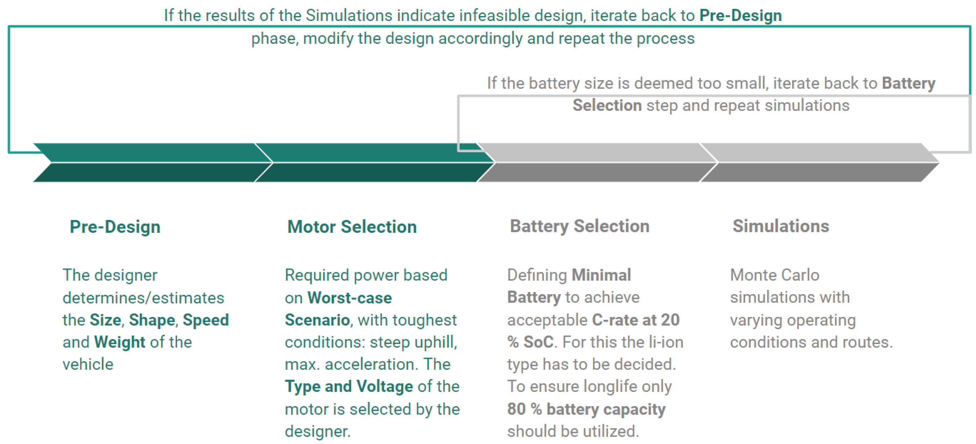
The purpose of this study is to dimension the electric powertrain components for a high-speed delivery robot. The powertrain components of interest in the preliminary design of an electric vehicle are the motor and the battery. In Figure 1, the steps of powertrain design are displayed. The preliminary size and shape of the SADR are dependent on the size of the packages it deliveres. The second step of powertrain design is to dimension the motor(s) of the SADR based on worst-case scenario load, similarly as in [21]. Next, minimum battery size is determined based on the C-rate of the battery and power at 20% state-of-charge in the worst-case scenario, which depends on the selection of the li-ion battery type. The battery C-rate is a metric used to describe the rate at which the battery is charged or discharged. The rate of 1C equals to a discharge current at which the battery is depleted in an hour. With a motor and battery size determined, Monte Carlo simulations are carried out to analyze the operation performance of the SADR. The Monte Carlo simulations determine how many cycles can be driven with a single charge of the battery. If the range of the vehicle is less than desired, battery size is re-calibrated and the simulations are rerun. If the range is altogether unacceptable, then the next design iteration starts from the beginning.

Figure 1.
Iterative design process of a powertrain. Multiple iterations of the process improve the design. The whole process does not have to be repeated if only the battery size is infeasible.
3.1.1. Pre-Design
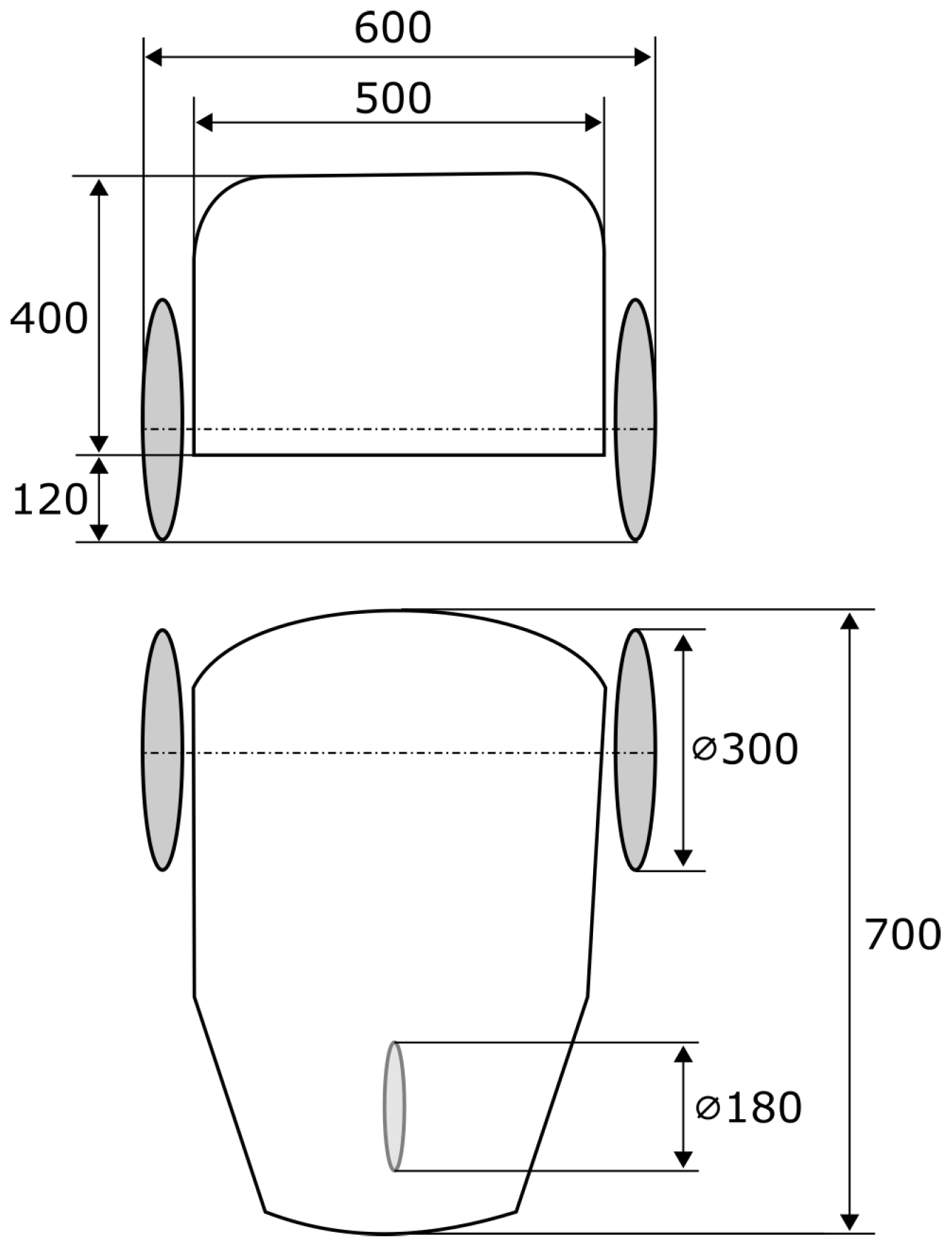
Here, a differential wheeled robot with two driving wheels with hub motors is considered, which translates to inexpensive and robust design. A sketch of the design is shown in Figure 2, where the third smaller wheel is a free turning wheel. The large front wheels allow the robot to travel in uneven terrain and hopefully climb sidewalk curbs. The maximum speed of the vehicle is set to 15 km/h so that it is within the Finnish and most of U.S. regulations [3,5]. The robot, including its body, electronics, wheels, motors and minimal battery, is estimated to weigh 16 kg. Based on the design, the frontal area is approximately 0.2 m and the coefficient of drag is 0.6.

Figure 2.
Preliminary design of the vehicle.
3.1.2. Motor Selection
The voltage level of the motor has to be determined by the designer. In a small vehicle such as a SADR, a low voltage level, such as 24, 36 or 48 V, is preferred which reduces the risk of serious electric shocks. In the worst-case scenario, the robot is accelerating to its maximum speed on an uphill, with its maximum load, headwind, and with snow or rough terrain that increases the rolling resistance coefficient. Tire slip is not considered. The robot dynamics and energy consumption are calculated with
In the equations above, are the resistive forces of movement, namely accelerative, drag, rolling resistance and slope, respectively. Mass is denoted as m, acceleration as a, velocity as v, coefficient of drag as , rolling resistance coefficient as , frontal area as A, density of air as , slope in degrees as , gravitational acceleration as g and the cumulative energy consumption in watt-hours is denoted with . The robot model is a backward-facing model, which means that the robot is assumed to follow the speed profile exactly and the energy consumption is calculated based on that behavior. Another possibility is to use a forward-facing model, which has the speed profile as a reference and the vehicle tries to achieve it using controllers. Forward-facing models are more complex and require more computational power but often offer more realistic results. Considering the computational load of thousands of simulations in this research, the backward-facing model was selected.
3.1.3. Battery Selection
The battery selection is dependent on the motor voltage and peak power, as they determine the peak C-rate. In addition, as a secondary condition, the charging C-rate should be considered. The charging power depends on the rate of charging, whether it is fast or slow charging. The capacity of the battery depends on the choice between opportunity or overnight charging. In opportunity charging, the battery is fast-charged at public chargers placed inside vendor facilities or out in the street, whenever an opportunity arises. In overnight charging, the battery is slowly charged at same places as for opportunity charging or at a robot depot at the end of the day, during nighttime. The available battery capacity and C-rate of the battery can be computed with
where is the battery capacity (in ampere-hours) reported in the datasheet, is the nominal voltage of the battery and is the maximum power of the motor. It is important to note that the battery should not be discharged under 20% State-of-Charge (SoC), for safety and longevity of the battery use. Therefore, only 80% of the battery capacity can be used and the battery has to be able to provide sufficient power at 20% or even 10% (rare cases) SoC. The maximum power of the motor in Equation (7) can be replaced by the power of charging to determine the C-rates of slow and fast charging. The battery design begins by selecting the smallest capacity battery possible because battery price is the most common economic feasibility issue along with weight and carbon footprint of manufacturing. After the minimum battery selection, operation of the robot is investigated with Monte Carlo simulations to determine the feasibility and possible need for a larger battery.
3.1.4. Simulations
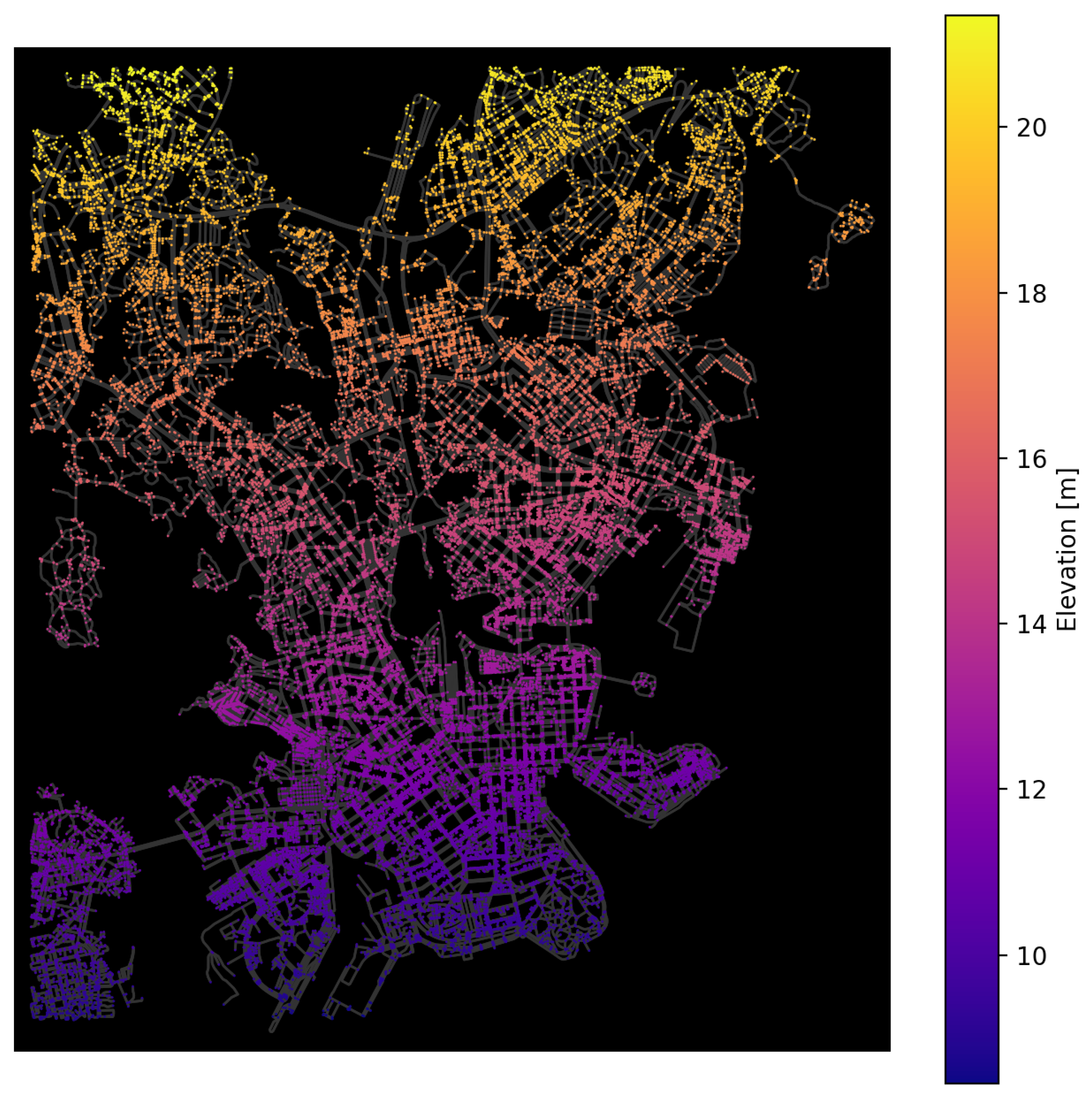
In the Monte Carlo simulations, synthetic operating cycles were generated based on delivery data acquired by Wolt [34]. These 18,500 deliveries were recorded in Helsinki, Finland, from August to September 2020. Open Street map is utilized with the Python library OSMnx [35] to determine the shortest routes for pedestrians from one location to another. The map consists of edges and nodes as shown in Figure 3. The synthetic cycles are generated from the pedestrian route provided by OSMnx with user and vendor locations as inputs. OSMnx returns a list of edges and their lengths.

Figure 3.
Map of Helsinki pedestrian routes based on the OpenStreet map Python package OSMnx [35], covering the area of all of the deliveries in the Wolt delivery dataset. The colored nodes are intersections and grey lines are edges connecting them. The color of the map indicates the elevation, which was acquired with open source Open Topo Data API [36].
Simulated stops are added to the route with the probability of 10% for each node as it resulted with an estimated realistic amount of stops per kilometer. If no stop occurs, the length of two edges are added together. On each of the edges, the robot is given one third of the edge length for acceleration. Then, the robot tries to reach its maximum speed but will settle for a lower speed if there is no time to achieve it. Idle time is added after each stop. Idle is the time spent on a stand-still whenever the robot has stopped, which is supposed to simulate the wait for crossing, traffic lights or a crowd to clear in front of the vehicle. The acceleration, deceleration and idle values are drawn from truncated Gaussian distributions. In addition, the mass, headwind, rolling resistance coefficient and auxiliary power are also uncertain factors with Gaussian noise. The input factor distributions are shown in Table 1.

Table 1.
Distributions of the uncertain input factors. The distributions are estimates and are not based on measured data. The distributions are truncated to within the bounds of minimum and maximum values.
3.2. Energy Demand
3.2.1. Energy Distribution
The energy demand of the robot consists of the power required for accelerations, uphill driving, auxiliaries, rolling resistance, aerodynamic drag, and motor and battery losses. Energy distribution among these factors was analyzed based on the energy spent per factor on each trip in relation to the entire energy spent on the trip. Then, the average was calculated from 5000 Monte Carlo simulations. The energy contribution of each power loss source is estimated as
where is the energy spent by the ith factor, is the total energy consumption, is the expected value and N is the number of simulations.
3.2.2. Sensitivity Analysis
Sensitivity analysis is the investigation of which input factor’s uncertainty causes the most uncertainty in the energy demand. Variation is the quantitative measure of uncertainty. The variation of the output depends on the input factor variation. Variation in the energy demand affects the range and battery sizing of the robot. The output variance is also referred to as unconditional variance of the system. The delivery robot model can be portrayed as a function
where is the ith input and y is the system output. Uppercase letters Y and X are used to refer to output array and input matrix consisting of rows of observations. Variance-based sensitivity approaches are typically utilized in global sensitivity analysis, where all of the system inputs are varied simultaneously in their full range of variation, opposed to local sensitivity analyses where one factor is varied at a time and/or only small variations are considered in the input factors. The sensitivity of the system to a single factor’s variation is quantified with a standardized metric called Sobol’s indices, which are calculated as
where is the first-order sensitivity index, is the partial variation contribution of the ith factor, is the expected value and is the variation. Sobol’s sensitivity indices indicate the effect of input factor variation to the output variation [37,38]. The first-order effect is the independent contribution of an input factor. The sum of first-order sensitivity indices is always less than or equal to unity, as unity resembles the entire variation of the output. If the sum of first-order effects is unity, the system is referred to as additive. In case there are high-order effects, the sum of first-order effects is less than unity and the system is therefore non-additive.
The total effect, measured by the total sensitivity index , is the entire contribution of an input factor, including the first-order effect in addition to high-order effects. The total sensitivity index is calculated as
where refers to all-but-i. The contribution of interaction effects are measured by discounting the variation caused by the independent effects, and , from their interaction sensitivity index
where is the variation caused only by the interaction of factors and . By including higher-order effects, such as , the sum of sensitivity indices sum is always equal to unity
where k is the number of factors. This statement holds when all of the sensitivity effects are orthogonal and thus uncorrelated. The original function can be decomposed as a high-dimensional model representation (HDMR)
The expression can be also written as a variance decomposition, also known as the analysis of variance (ANOVA) decomposition
where p is a subset of 1, 2, …, k as denoted originally in [39], with .
The HDMR was first introduced by Rabitz [40]. Sobol’s built on his work for calculating global sensitivity indices based on HDMR that are now referred to as Sobol’s sensitivity indices [37]. In many cases, such as the one here, there is no control over some of the variables (elevation, time and distance of trips). Therefore, there can be correlations amongst the input factors which violate the rules behind Equations (13)–(15), which expect the input factors to be orthogonal and uncorrelated. Xu and Gertner presented a method to calculate the sensitivity indices while correlations are present for a linear model [41]. Li et al. built on their work and proposed an approach for calculating sensitivity indices using random sampling-HDMR (RS-HDMR), which includes nonlinearities and higher-order effects with independent and/or correlated inputs [39]. A more general ANOVA decomposition is the analysis of covariance (ANCOVA) decomposition
where is the covariance and is a random error [41]. If the is small compared to , the estimation of sensitivity indices is a good approximation. Since the correlated effect is the covariance of two factors, it can assume negative values. In the presence of correlations, the sensitivity of one or a subset of input factors cannot be described with a single sensitivity index. Instead, the sensitivity of a single factor is decomposed further based on Equation (17), which are
total, structural and correlative contributions, respectively [39].
The SALIb implementation of RS-HDMR meta-modeling input-output data is utilized here, which uses cubic B splines to approximate the sub-functions of HDMR [39,42]. The coefficients are calculated by using a backfitting procedure utilizing the statistical F-test for identifying meaningful sub-functions and neglecting the rest from the HDMR [39]. An estimated 95% confidence is given for the sensitivity indexes based on bootstrapping. For the bootstrapping, 20 iterations are made with randomly chosen N/2 observations. Repetition is allowed in the randomization. A total of 18,000 simulations were run with uniform distributions of the inputs listed in Table 1. Drawing values from uniform distributions explores the parameter space more efficiently than with Gaussian distributions, as it is less unlikely for a factor to vary drastically from its expected value. As the elevation, time and distance of a trip are random, more efficient pseudo-sampling techniques such as Latin hypercube, Sobol’s or Halton sampling were not considered for the sake of equal treatment of the input factors.
3.3. Cost of Transport
There are no published works or metrics of wheeled robots, such as Kiwi, Starship and Scout, except for their speed and weight. Starship has an unofficial public datasheet which is utilized here for the estimations [10]. Since they are miniature electric vehicles, their cost of transport (CoT) should resemble that of a miniature car. Multiple quadruped robots are also considered in the comparison, since they could be potentially used for deliveries as well with the capability to travel in difficult terrain and stairs. Few quadruped animals (German Shepherd, cheetah and horse) are considered in the analysis as comparison for the capabilities of biological systems. CoT is a unitless metric that only takes into account the energy required for locomotion. It is used here to compare the energy efficiency of biological and robotic systems. CoT is defined as
where the ratio of the total energy consumption E for a travel of a distance d regarding the gravitational force (mass m times gravitational acceleration g) or by the input power P divided by constant velocity v [43]. It is important to note that only the energy or input power used for locomotion is accounted for and not even traction-related auxiliary power is included. This means that the lower the CoT, the higher the locomotion energy efficiency. For example, human running is less efficient than walking, since a human of 70 kg walks at 0.38 CoT (1.75 m/s) and jogs (3.75 m/s) with 0.47 CoT [43]. Energy consumption is referred here as the energy of transport (EoT), which is CoT in the units of watt-hours per kilometer in addition to the the auxiliary power, . EoT is defined as
where is the vehicle speed in kilometers per hour.
4. Results
4.1. Powertrain Design
4.1.1. Iteration 1: Minimal Battery
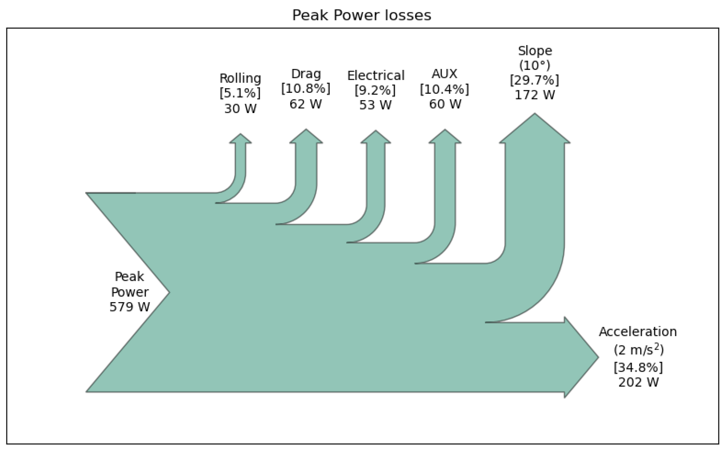
Worst-case scenario analysis is used to dimension the hub motors of the robot. In this scenario, the robot drives with an acceleration of 2 m/s until it reaches 15 km/h, it is facing a headwind of 10 m/s, carrying maximum capacity package of 8 kg, on rough terrain with a rolling resistance coefficient of 0.03 and a slope of 10 degrees uphill. In Figure 4, the peak power distribution at the end of the acceleration is displayed with a Sankey diagram.

Figure 4.
Power distribution with minimal battery (166 Wh and 1.1 kg).
The motors should provide a total of 520 W of power together, since auxiliary power is not provided by the motors. Hence, two 250-W motors should suffice, since motors can be used momentarily with power that exceeds their reported peak power. Even 200 W could be considered if acceleration in an uphill is not a priority, since the peak power demand while accelerating on flat ground is 350 W.
A minimal battery of 4500 mAh LiPo (Lithium-polymer battery) pack 35C is selected [44]. The battery pack consists of 10 cells of nominal voltage of 3.7 V in series and has an energy density of 120 Wh/kg. The motor nominal operating voltage should therefore also be 36 V. Capacity of the battery is 166 Wh but only 80% of the capacity is used to ensure long lifetime of the battery. At 20% SoC, the battery voltage is estimated to be 34 V and maximum power consumes 17 A, resulting in a C-rate of 3.8. This C-rate is an order of magnitude lower than the rated maximum C-rate of this particular battery. Slowly charging the battery with 500 W takes about 15 min and a fast charge with 2000 W can be done in 3 min. With the motors and battery selected, next, the Monte Carlo simulations are run.
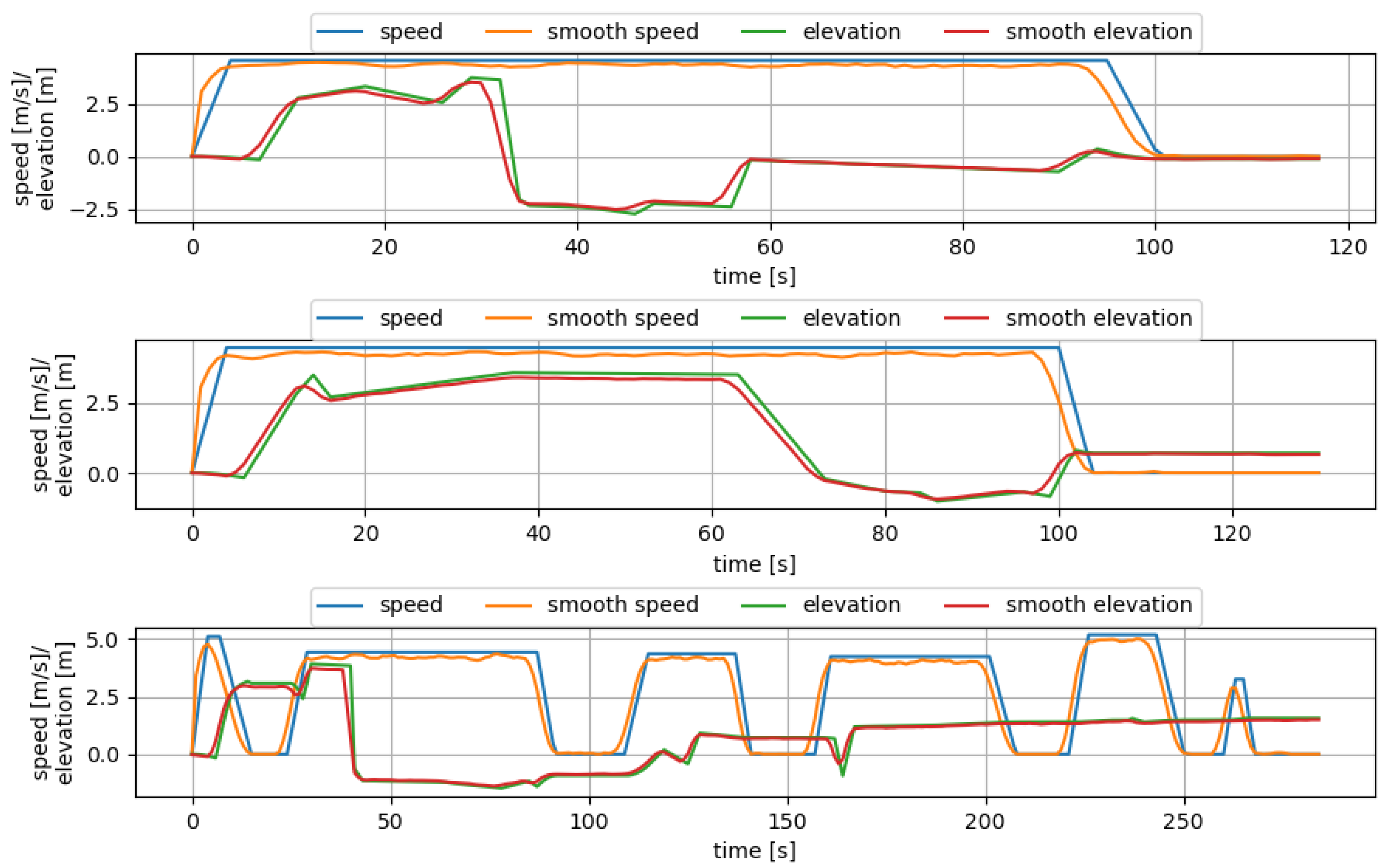
In Figure 5, examples of the generated synthetic driving cycles are shown. Auto-correlated noise and moving-average are added to smooth the speed and elevation, as an attempt to make the cycles more realistic. A total of 5000 synthetic cycles were selected randomly from the available 18,500 trip dataset. The average energy consumption of the simulated cycles was 6.5 Wh/km. Energy and time spent per trip on average was 8.4 Wh and 5.8 min, respectively. With the minimal battery, there is enough energy for approximately 18 trips, which translates to a driving time of 1.4 h and a range of 19 km. It should be noted that the transition from last trip destination to next trip origin are not considered when calculating the number of total trips.

Figure 5.
Random samples of the generated synthetic driving cycles. Blue and green indicate the speed and elevation profiles without noise. Orange and red are the smoothed signals with the use of auto-correlation and moving-average algorithms.
4.1.2. Iteration 2: Full-Day Battery
Based on the simulations, a minimal battery has sufficient capacity for carrying out the delivery task. For comparison, another iteration is studied where the battery capacity is large enough for the robot to operate all day and only charge during the night. Operation time of 12 h is estimated to suffice for full-day operation with one charge. Based on the previous calculations, eight pieces of the “minimal batteries” are added in parallel. This increases the battery capacity significantly, but also the battery weight.
The worst-case scenario is the same as with the minimal battery except the battery weighs 9 kg instead of 1 kg. In this case, the motors should provide a total of 670 W of power together. Hence, two 350 W motors should suffice, even 250 W could be considered if acceleration in an uphill is not a priority, since the peak power demand while accelerating on flat ground is 440 W. With eight batteries in parallel, the utilizable battery capacity is 1065 Wh. At 20% SoC, maximum power consumes 20 A, resulting in a C-rate of 0.6. The lower C-rate compared to the minimal battery is likely to increase the lifetime of the battery. Slow charging the battery with 500 W takes about two hours and a fast charge with 2000 W takes half an hour. Hence, for eight hour overnight charging, as low as 125 W power can be considered.
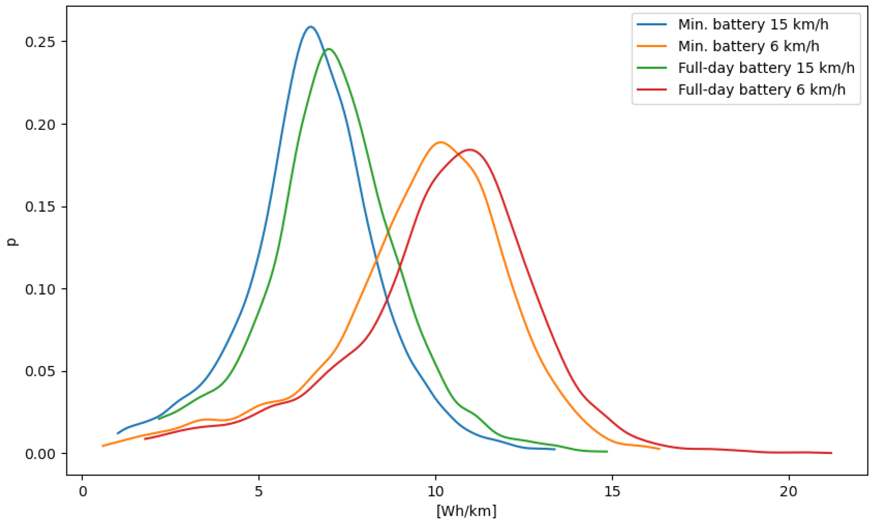
In the Monte Carlo simulations, the average energy consumption of the simulated cycles was 7.1 Wh/km. Energy and time spent per trip on average was 9.2 Wh and 5.8 min, respectively. With the minimal battery, there is enough energy for approximately 115 trips, which translates to a driving time of 11.2 h and a range of 150 km. It should be noted that the transition from last trip destination to next trip origin are not considered when calculating the number of total trips. In Figure 6, the energy consumption distribution with a minimal and full-day battery are presented. The probability density functions of energy distributions were generated using Kernel Density Estimation. In addition, low-speed operation with a maximum speed of 6 km/h with both battery packs was also considered to demonstrate the benefit of higher speed operation.

Figure 6.
Energy consumption distribution with both minimal and full-day batteries, and high-speed (15 km/h) and low-speed (6 km/h).
The energy consumption is only slightly higher with the full-day battery than with the minimal battery, even though there is a significant weight difference. In addition, the variation in energy consumption was larger when operating at a lower maximum speed. The smaller battery is suitable for less than 1.5 h of operation, whereas a larger battery enables for over 11 h of operation. It is clear that faster operating speed results in significantly lower energy consumption. The choice between selecting the low or high capacity battery depends on the battery price, charging station price and placement, and the hilliness of the area. In Table 2, the comparison of the minimal and full-day batteries and operation is summarized.
Table 2.
Comparison of minimal and full-day batteries when operating at high-speed (15 km/h).
4.2. Energy Demand
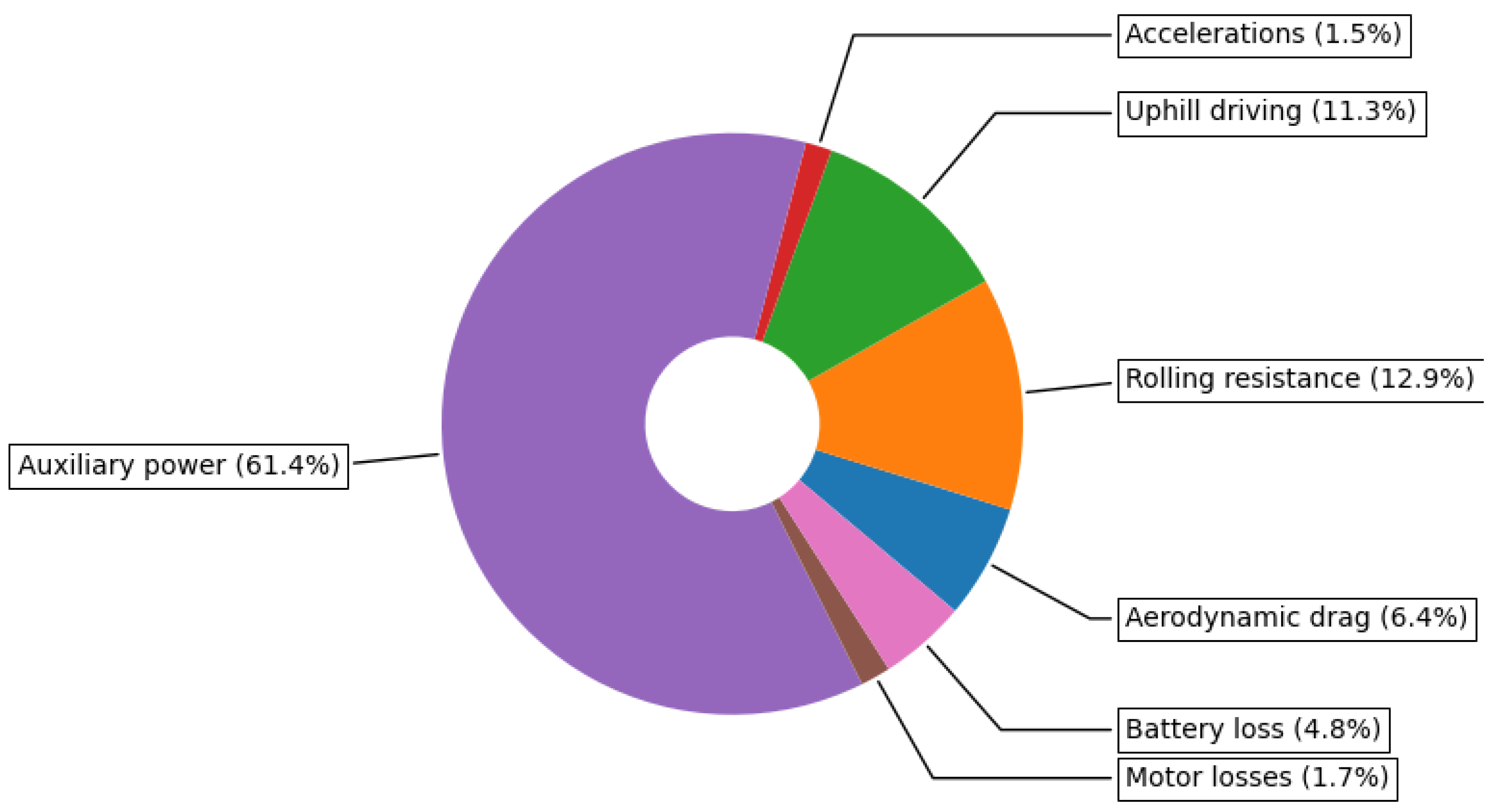
The energy demand of the robot consists of the power required for accelerations, uphill driving, auxiliaries, rolling resistance, aerodynamic drag, and motor and battery losses. Based on 5000 simulations, the average energy demand distribution is presented in Figure 7. Clearly, most of the energy is spent for auxiliary power with more than 60% share of the average energy demand. The power of computation for sensing and control in a small vehicle such as a delivery robot is a crucial aspect, as the energy required for traction is minuscule. Rolling resistance and uphills together account for almost 25% of the energy demand. The contribution of uphills could be much higher in some other geographical locations as Helsinki is a relatively flat area. Good road and tire maintenance could also decrease the energy demand.

Figure 7.
Average energy demand distribution during operation.
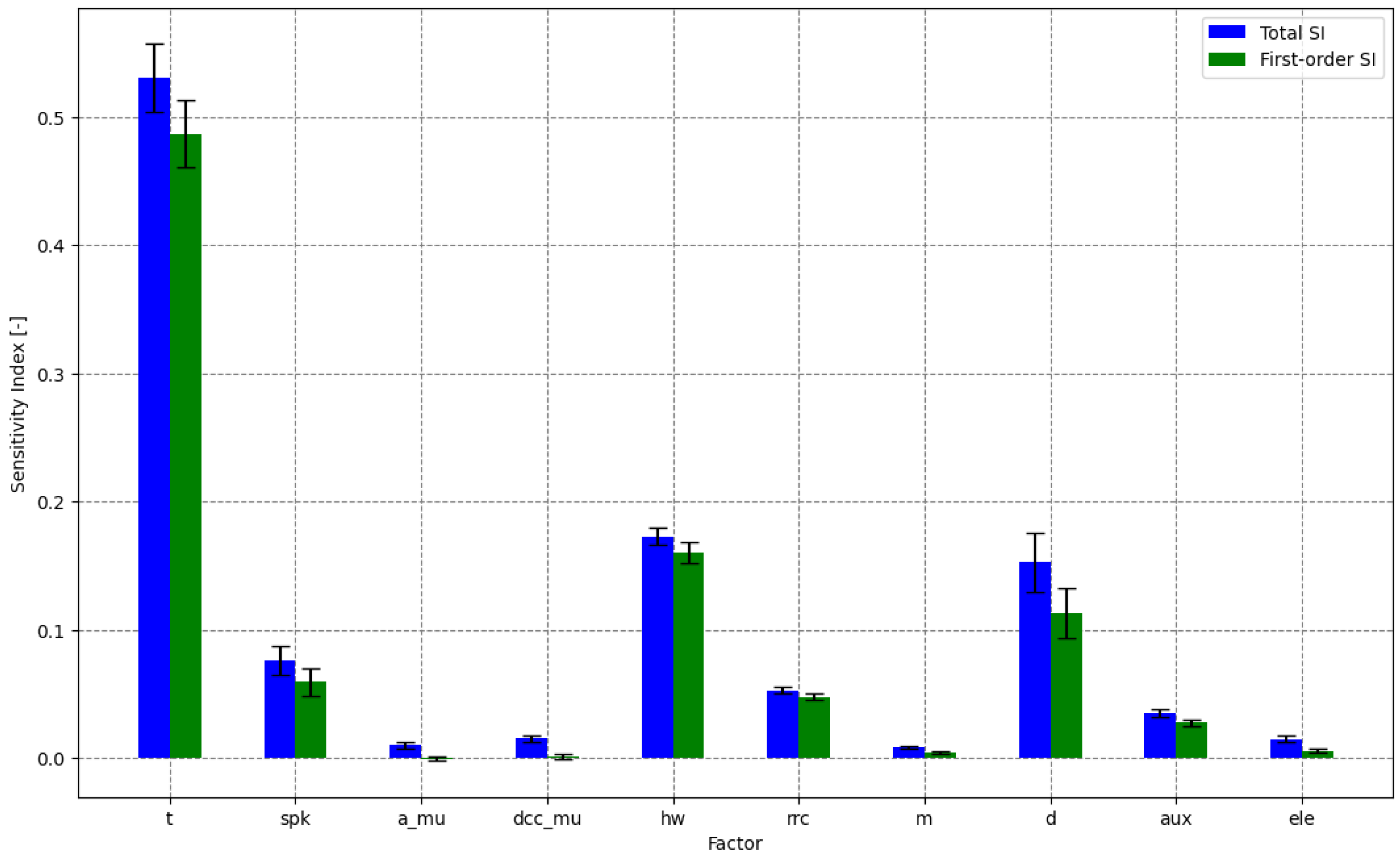
In addition to average energy demand, the variation in energy demand and its key sources were investigated. The variation of energy consumption can be seen in Figure 6, which is lower with higher speed and vice versa. The investigation of most significant contributors to the energy demand variation were investigated with a variance-based global sensitivity analysis. The first-order and total sensitivity indices for energy spent per kilometer driven are shown in Figure 8.

Figure 8.
Total and first-order sensitivity indices. The input factors considered in the analysis were: t = time, spk = stops per kilometer, a_mu = mean acceleration, dcc_mu = mean deceleration, hw = headwind, rrc = rolling resistance coefficient, m = payload mass, d = distance, aux = auxiliary power and ele = elevation.
The sum of first-order sensitivity indices was 0.91 and, thus, correlations and interaction effects played a minor role in the variation contribution; however, it is mainly driven by the first-order effects. The error bounds of the sensitivity indices were calculated with bootstrapping, which indicate that the results are a good approximation of the variance decomposition. Variation in the time (t) spent on route had the most significant effect as the longer time is spent on idle, the higher the energy consumption per kilometer due to the non-traction-related auxiliary power consumption.
Surprisingly, headwind () had the second most largest effect on energy variation, which had one third of the contribution of trip time variation. Route distance (d) variation had a similar effect as headwind. On short routes, there are only a few or even no stops which reduce idle time and energy spent on accelerations. Stops per kilometer () variation had only a small effect, but the more stops there are, the more idling and accelerating there are as well. Rolling resistance () and auxiliary power () variations had only a small effect on energy demand. It is interesting how the contributions of rolling resistance and headwind are reversed when it comes to the average energy demand contribution and the contribution to the variation of energy demand. It could be that the rolling resistance average value is already high and variation is small and vice versa for headwind. Auxiliary power variation seems to have a surprisingly small effect. It would seem that the energy demand variation is not driven by the exact value of auxiliary power but rather the duration of its use. Furthermore, the auxiliary power was considered as a constant value for the trip, which most likely is not the case in reality. Auxiliary power could be significantly lower on idle compared to moving in highly crowded places. Variation in acceleration, deceleration, payload and elevation had insignificant effects on the energy demand variation.
4.3. Cost of Transport
In addition to energy demand analysis, the cost of transport and carbon footprint of deliveries were also studied. The high-speed delivery robot was compared to state-of-the-art wheeled robots. In addition, quadruped robots and animals were also considered in the analysis, to provide a perspective of their performance and energy efficiency. Since there was limited information available of multiple robots, the CoT and energy consumption values are in some cases estimated by the author based on the limited data. The results of the analysis is shown in Table 3, in which the designed robot in this paper is referred to as D-bot and it is equipped with the full-day battery. The high-speed D-bot has the best energy efficiency of all of the considered robots. It must be highlighted that the results of this paper are based on synthetic cycles and simulations, whereas the performance of some of the considered robots is based real-world measurements and some are based in mere estimations. A good example is that the low-speed D-bot has only half of the consumption of the Starship, even though they have similar weight and speed. This is probably due to the fact that many factors, such as climbing curbs, wheel slips, suspension, battery and motor dynamics, and thermodynamics, were not considered in the simulation model.
Table 3.
Cost, energy and carbon footprint of transport and delivery of robots and few mammals.
Starship has an energy consumption of roughly 20 Wh/km, which is similar to that of an electric bicycle [47]. The quadruped that comes close to this is Spot with roughly thrice as high energy consumption. The MIT-Cheetah III has very similar carbon footprint of delivered kilogram as Spot. Spot and MIT-Cheetah III are both mammal-type quadrupeds. The only sprawler-type quadruped considered here, the TITAN-XIII, has an energy consumption of only almost half of Spot’s, but adding load to it increases the energy consumption significantly. ALPHARED has the possibility of utilizing caster wheels instead of walking, which greatly increases energy efficiency but is still far from the efficiency of Spot and MIT-Cheetah III. BigDog is the only robot considered that is powered by an internal combustion engine and that translates to a high energy consumption. The CoT of animals is similar to that of the best performing quadrupeds. Wheeled robots would seem to be the only ones to reach better efficiency, at least based on these estimations.
5. Discussion
The proposed powertrain design approach was shown to be a useful and systematic tool in the design process of a new vehicle application. However, in its current form, it only considers battery electric powertrains. Hybrid electric powertrains could also be considered, where the electric powertrain is coupled with an internal combustion engine, fuel cell stack, flywheel, etc. In addition, the inclusion of other forms of transportation, such as trains, planes and ships, would enhance the generality of the approach. The results of the designed delivery robot are promising but real-world tests must be conducted in order to validate them. Measured driving cycles could be used for the simulations instead of synthetic ones to improve the reliability of the results. However, before a system is built, it is impossible to measure data of it and, thus, synthetic cycles offer a means to an end. The robot model is a system level backward-facing model, which is fast to compute and is therefore practical for a large number of simulations. The use of a backward-facing model might lead to scenarios where the robot behaves unrealistically, e.g., the robot accelerates in an uphill faster than it actually could.
A higher fidelity model, which would be forward-facing and include wheel slip, suspension, battery and motor dynamics, and thermodynamics, could provide more accurate results. The simplistic model could be the reason behind the fact that the low-speed D-bot had half the energy consumption of Starship, even though they have similar weight and speed. However, increasing the fidelity of the model should be based on comparison and validation against real-world measurement data, not the simulations and estimations made in this study. Constant efficiency was used here to model the dynamic behavior of the battery. Including the battery dynamics with a Thevenin model would introduce the dynamics of the voltage and current, which means that the battery would no longer be modeled with a constant efficiency and instead the losses would be modeled based on an internal resistance voltage drop. Similarly, the motor could be modeled based on dynamics of a 3-phase motor; however, it was not for the sake of faster computation. Both the battery and motor could also be modeled based on efficiency maps, which would not increase computation significantly; yet, it would increase the accuracy of the model. Furthermore, energy regenerative braking could be studied by introducing a detailed electric drive model.
Low-speed operation was considered as a comparison to show the benefits of higher operating speeds. It was shown that the difference in energy consumption between low- and high-speed operation was significant, while the increase in battery size had only a small impact. The energy demand variation was also higher with lower speeds. However, legislation and regulations still restrict higher speeds of delivery robots in some locations. With the minimal battery, there is enough energy for operation of 18 trips that take approximately 100 min. However, the transitions between delivery destination and next delivery origin were not considered here. Including the transitions in future research would enable the comparison of human and robot delivery operation. Thus, probably 10 deliveries can be made with one charge. The slow charging of the minimal battery is 15 min, so the downtime is reasonable in comparison to uptime. Fast charging is also a possibility, with a charge of only 3 min, which can be utilized during periods of high demand. However, the minimal battery requires chargers installed in many places, possibly on the street, inside restaurants or next to the postal lockers. A full-day battery enabled the robot to operate throughout the day and very slow charge during the night, which increases the lifetime of the battery. The choice between a minimal and full-day battery depends also on the business model of the delivery company, cost of charging stations and cost of battery capacity.
In the energy demand analysis, the auxiliary power was shown to contribute most to the average energy demand during trips. To improve the energy efficiency, lower computation control and monitoring methods should be considered, even though the auxiliary power is already relative low, comparable to a light bulb. The energy demand was most sensitive to variation in trip time because auxiliary power, as the energy of auxiliaries spent per kilometer is infinite when idling. Therefore, not only is rapid delivery with minimal stops and idling preferable for the customer but also for the sake of energy efficiency. Furthermore, the energy demand variation is not driven by the exact value of auxiliary power but rather the duration of its use. Furthermore, the energy consumption would be probably higher with more local elevation variation. In Figure 3, the elevation slowly increases while moving from south to north and there are practically no clear inconsistencies due to smaller hills. The open source elevation API (Open Topo Data) employed here has a resolution of 25 m in Europe. Using a paid API such as Google’s elevation, API would increase the accuracy of the elevation profile as they provide a resolution of as low as 5 m. The comparison of energy consumption and the carbon footprint of robots gives an insight to which robot designs and locomotion styles are the most suitable for delivery robots. However, the comparison is based on estimations. In order to accurately determine the presented metrics, future studies should focus on testing identical deliveries carried out with various robots.
6. Conclusions
In this paper, a novel step-by-step powertrain design approach is proposed. It is is based on performance requirements, which are divided into powertrain and operation requirements in the literature. The approach is meant for new vehicular and mobile robot applications, where previous data of the operation are unavailable. The process consists of pre-design, motor selection, battery selection and Monte Carlo simulation phases. First the size, shape and speed of the vehicle are estimated according to the application, followed by motor selection based on operation in worst case conditions. Then, the minimum capacity of the battery is determined which is capable of supplying the peak power for the motor. Minimal battery is preferred because it minimizes its cost, weight and carbon footprint. Then, Monte Carlo simulations are run with synthetic driving cycles which are based on open street map routing. This process is iterative. If the simulations show that the whole design is unfeasible, one should iterate back to the beginning. However, if only the battery is too small, only the battery capacity and weight can be updated and, then, the simulations can be rerun. Energy demand and its variation analysis are also a part of the proposed powertrain approach. This analysis is the investigation of which factors contribute most to energy demand and its variation. Crucial factors can then be identified and used to enhance the design and lower the variation of energy demand.
The design process was shown to provide satisfactory results in the case of designing a delivery robot. Initially, a powertrain with minimal battery was designed, which enabled the robot to operate one and half hours with one charge. Then, a larger capacity battery design was introduced, one which could operate throughout the day with a single charge. Monte Carlo simulations were carried out using synthetic cycles using the start and end coordinates of the Wolt dataset consisting of deliveries in Helsinki, Finland. Based on the simulations, it was shown that significant addition of battery weight of higher capacity battery did not increase energy consumption significantly. However, the operation speed had a significant impact on the energy demand. When the maximum speed was 15 km/h, the energy consumption was reduced more than 40% in comparison to operation with a maximum speed of 6 km/h. Energy demand analysis showed that more than half of the energy is spent on auxiliary power demand. The variation in energy demand was mainly caused by changes in trip time, as longer trip time resulted in more idling and more stops due to crossings and crowds. The designed robot is energy efficient when compared to the existing wheeled and quadruped robots. However, the comparison was based on limited available data and, thus, some of the metrics had to be estimated.
In future work, the proposed approach should be extended to include models of other forms of locomotion, such as trains, planes and ships. In addition, the robot model should be validated against real-world experiment data. The battery and motor could also be modeled more in detail to increase the accuracy and enable the study of regenerative braking control. Auxiliary power consumption was a major contributor to energy consumption, thus using sleep-mode for sensors and computation hardware should be studied. Furthermore, a fair comparison between robots should be carried out with experiments that include identical deliveries carried out with various robots. The success of delivery robots in particular not only depends on the energy efficiency but also on the public acceptance. A better efficiency robot might not be as widely accepted as another that is more aesthetically pleasing or which behaves in a way that better blends in with the people flow.
Funding
This research received no external funding.
Data Availability Statement
The code implementations presented in the paper are available at the following open source repository, created by the author: https://github.com/vepsalai/high-speed-delivery-robot (created on 14 February 2022).
Conflicts of Interest
The author declares no conflict of interest.
Abbreviations
The following abbreviations and mathematical symbols are used in the paper. Abbreviations are listed in alphabetical order and the symbols in the order of appearance.
| ADR | autonomous delivery robot |
| ANCOVA | analysis of covariance |
| ANOVA | analysis of variance |
| aux | auxiliary power |
| CoT | cost of transport |
| dcc | deceleration |
| DOF | degrees of freedom |
| EoT | energy of transport |
| HDMR | high-dimensional model representation |
| hw | head wind |
| idle | idle time |
| rrc | rolling resistance coefficient |
| RS-HDMR | random sampling-high-dimensional model representation |
| SADR | sidewalk autonomous delivery robot |
| SEA | series elastic actuator |
| SoC | State-of-Charge |
| force for acceleration (Newton’s 2nd law of motion) | |
| resistive force of aerodynamic drag | |
| resistive force of rolling resistance and slope | |
| m | mass |
| a | acceleration |
| v | velocity |
| coefficient of drag | |
| rolling resistance coefficient | |
| A | frontal area |
| density of air | |
| slope (in degrees) | |
| g | gravitational acceleration |
| cumulative energy consumption in watt-hours | |
| available battery capacity | |
| battery capacity (in ampere-hours) reported in the datasheet | |
| C-rate of the battery | |
| nominal voltage of the battery | |
| maximum power of the motor | |
| energy contribution of each power loss source (estimate) | |
| energy spent by the ith factor | |
| total energy consumption | |
| expected value | |
| N | number of simulations |
| function | |
| ith input | |
| y | system output |
| Y | output array |
| X | input matrix |
| first-order sensitivity index | |
| partial variation contribution of the ith factor | |
| variation | |
| total sensitivity index | |
| variation caused only by the interaction of ith and jth factor | |
| k | number of factors |
| p | subset |
| covariance | |
| Gaussian random error | |
| total sensitivity contribution | |
| structural sensitivity contribution | |
| correlative sensitivity contribution | |
| E | energy consumption |
| d | traveled distance |
| P | input power |
| auxiliary power | |
| speed in kilometers per hour |
References
- Dolan, S. The Challenges of Last Mile Delivery Logistics and the Tech Solutions Cutting Costs in the Final Mile. Business Insider. 2021. Available online: https://www.businessinsider.com/last-mile-delivery-shipping-explained?IR=T (accessed on 1 March 2021).
- Joerss, M.; Schröder, J.; Neuhaus, F.; Klink, C.; Mann, F. Parcel Delivery: The Future of Last Mile; McKinsey & Company: Brussels, Belgium, 2016; pp. 1–32. [Google Scholar]
- Jennings, D.; Figliozzi, M. Study of sidewalk autonomous delivery robots and their potential impacts on freight efficiency and travel. Transp. Res. Rec. 2019, 2673, 317–326. [Google Scholar] [CrossRef] [Green Version]
- Finnish Government Proposal (HE 180/2017), Section 3.2.1. Finlex. 2020. Available online: https://www.finlex.fi/fi/esitykset/he/2017/20170180 (accessed on 15 March 2021).
- Finnish Road Law (729/2019) 52 §, 99 §. Finlex. 2020. Available online: https://www.finlex.fi/fi/laki/ajantasa/2018/20180729 (accessed on 15 March 2021).
- Hooks, J.; Ahn, M.S.; Yu, J.; Zhang, X.; Zhu, T.; Chae, H.; Hong, D. Alphred: A multi-modal operations quadruped robot for package delivery applications. IEEE Robot. Autom. Lett. 2020, 5, 5409–5416. [Google Scholar] [CrossRef]
- Korosec, K. Kiwibot delivery robots head to San Jose with new partners Shopify and Ordermark. TechCrunch News. 21 July 2020. Available online: https://techcrunch.com/2020/07/21/kiwibot-delivery-robots-head-to-san-jose-with-new-partners-shopify-and-ordermark/ (accessed on 5 November 2021).
- Korosec, K. Starship Technologies is sending its autonomous robots to more cities as demand for contactless delivery rises. TechCrunch News. 9 April 2020. Available online: https://techcrunch.com/2020/04/09/starship-technologies-is-sending-its-autonomous-robots-to-more-cities-as-demand-for-contactless-delivery-rises/ (accessed on 5 November 2021).
- Nichols, G. Amazon delivery robots are officially on the streets of California. ZDNet News. 7 August 2019. Available online: https://www.zdnet.com/article/amazon-delivery-robots-are-officially-on-the-streets-of-california/ (accessed on 11 November 2021).
- Factsheet—Starship Delivery Robot. Swiss Post. 2020. Available online: https://www.post.ch/-/media/post/ueber-uns/medienmitteilungen/2017/factsheet-lieferroboter.pdf?la=en (accessed on 2 December 2021).
- Murgovski, N.; Johannesson, L.; Sjöberg, J.; Egardt, B. Component sizing of a plug-in hybrid electric powertrain via convex optimization. Mechatronics 2012, 22, 106–120. [Google Scholar] [CrossRef] [Green Version]
- Pourabdollah, M.; Murgovski, N.; Grauers, A.; Egardt, B. Optimal sizing of a parallel PHEV powertrain. IEEE Trans. Veh. Technol. 2013, 62, 2469–2480. [Google Scholar] [CrossRef] [Green Version]
- Pourabdollah, M.; Egardt, B.; Murgovski, N.; Grauers, A. Convex optimization methods for powertrain sizing of electrified vehicles by using different levels of modeling details. IEEE Trans. Veh. Technol. 2017, 67, 1881–1893. [Google Scholar] [CrossRef]
- Lei, F.; Bai, Y.; Zhu, W.; Liu, J. A novel approach for electric powertrain optimization considering vehicle power performance, energy consumption and ride comfort. Energy 2019, 167, 1040–1050. [Google Scholar] [CrossRef]
- Hegazy, O.; Van Mierlo, J. Particle swarm optimization for optimal powertrain component sizing and design of fuel cell hybrid electric vehicle. In Proceedings of the 2010 12th International Conference on Optimization of Electrical and Electronic Equipment, Brasov, Romania, 20–22 May 2010; pp. 601–609. [Google Scholar]
- Ebbesen, S.; Dönitz, C.; Guzzella, L. Particle swarm optimisation for hybrid electric drive-train sizing. Int. J. Veh. Des. 2012, 58, 181–199. [Google Scholar] [CrossRef]
- Soleymani, M.; Yoosofi, A.; Kandi-d, M. Sizing and energy management of a medium hybrid electric boat. J. Mar. Sci. Technol. 2015, 20, 739–751. [Google Scholar] [CrossRef]
- Schönknecht, A.; Babik, A.; Rill, V. Electric powertrain system design of BEV and HEV applying a multi objective optimization methodology. Transp. Res. Procedia 2016, 14, 3611–3620. [Google Scholar] [CrossRef] [Green Version]
- Anselma, P.G.; Belingardi, G. Comparing battery electric vehicle powertrains through rapid component sizing. Int. J. Electr. Hybrid Veh. 2019, 11, 36–58. [Google Scholar] [CrossRef]
- Lajunen, A. Powertrain design alternatives for electric city bus. In Proceedings of the 2011 IEEE Vehicle Power and Propulsion Conference, Chicago, IL, USA, 6–9 September 2011 2012; pp. 1112–1117. [Google Scholar]
- Grunditz, E.A. Design and Assessment of Battery Electric Vehicle Powertrain, with Respect to Performance, Energy Consumption and Electric Motor Thermal Capability; Chalmers Tekniska Hogskola: Göteborg, Sweden, 2016. [Google Scholar]
- Katz, B.G. A Low Cost Modular Actuator for Dynamic Robots. Master’s Thesis, Massachusetts Institute of Technology, Cambridge, MA, USA, 2018. [Google Scholar]
- Park, H.W.; Kim, S. The mit cheetah, an electrically-powered quadrupedal robot for high-speed running. J. Robot. Soc. 2014, 32, 323–328. [Google Scholar] [CrossRef]
- Raibert, M.; Blankespoor, K.; Nelson, G.; Playter, R. Bigdog, the rough-terrain quadruped robot. IFAC Proc. Vol. 2008, 41, 10822–10825. [Google Scholar] [CrossRef] [Green Version]
- Semini, C. HyQ-Design and Development of a Hydraulically Actuated Quadruped Robot. Ph.D. Thesis, University of Genoa, Genoa, Italy, 2010. [Google Scholar]
- Semini, C.; Barasuol, V.; Goldsmith, J.; Frigerio, M.; Focchi, M.; Gao, Y.; Caldwell, D.G. Design of the hydraulically actuated, torque-controlled quadruped robot HyQ2Max. IEEE/ASME Trans. Mechatron. 2017, 22, 635–646. [Google Scholar] [CrossRef]
- Yang, Y.; Semini, C.; Guglielmino, E.; Tsagarakis, N.G.; Caldwell, D.G. Water vs. oil hydraulic actuation for a robot leg. In Proceedings of the 2009 International Conference on Mechatronics and Automation, Changchun, China, 9–12 August 2009; pp. 1940–1946. [Google Scholar]
- Zhong, Y.; Wang, R.; Feng, H.; Chen, Y. Analysis and research of quadruped robot’s legs: A comprehensive review. Int. J. Adv. Robot. Syst. 2019, 16, 1729881419844148. [Google Scholar] [CrossRef] [Green Version]
- Kitano, S.; Hirose, S.; Horigome, A.; Endo, G. TITAN-XIII: Sprawling-type quadruped robot with ability of fast and energy-efficient walking. Robomech J. 2016, 3, 8. [Google Scholar] [CrossRef]
- Hutter, M.; Gehring, C.; Jud, D.; Lauber, A.; Bellicoso, C.D.; Tsounis, V.; Hwangbo, J.; Bodie, K.; Fankhauser, P.; Bloesch, M.; et al. Anymal-a highly mobile and dynamic quadrupedal robot. In Proceedings of the 2016 IEEE/RSJ International Conference on Intelligent Robots and Systems (IROS), Daejeon, Korea, 9–14 October 2016; pp. 38–44. [Google Scholar]
- Hutter, M.; Gehring, C.; Bloesch, M.; Hoepflinger, M.A.; Remy, C.D.; Siegwart, R. StarlETH: A compliant quadrupedal robot for fast, efficient, and versatile locomotion. In Adaptive Mobile Robotics; World Scientific: Singapore, 2012; pp. 483–490. [Google Scholar]
- Datasheet—Spot Explorer. Boston Dynamics. 2020. Available online: https://shop.bostondynamics.com/spot (accessed on 13 January 2022).
- Bledt, G.; Powell, M.J.; Katz, B.; Di Carlo, J.; Wensing, P.M.; Kim, S. MIT Cheetah 3: Design and control of a robust, dynamic quadruped robot. In Proceedings of the 2018 IEEE/RSJ International Conference on Intelligent Robots and Systems (IROS), Madrid, Spain, 1–5 October 2018; pp. 2245–2252. [Google Scholar]
- Wolt Enterprises, O. Data Science Summer Intern Assignment 2021. Available online: https://github.com/woltapp/data-science-summer-intern-2021 (accessed on 23 August 2021).
- Boeing, G. OSMnx: New methods for acquiring, constructing, analyzing, and visualizing complex street networks. Comput. Environ. Urban Syst. 2017, 65, 126–139. [Google Scholar] [CrossRef] [Green Version]
- Nisbet, A. Open Topo Data API. 2021. Available online: https://www.opentopodata.org/ (accessed on 5 January 2022).
- Sobol’, I.M. On sensitivity estimation for nonlinear mathematical models. Mat. Model. 1990, 2, 112–118. [Google Scholar]
- Saltelli, A.; Ratto, M.; Andres, T.; Campolongo, F.; Cariboni, J.; Gatelli, D.; Saisana, M.; Tarantola, S. Global Sensitivity Analysis: The Primer; John Wiley & Sons: Hoboken, NJ, USA, 2008. [Google Scholar]
- Li, G.; Rabitz, H.; Yelvington, P.E.; Oluwole, O.O.; Bacon, F.; Kolb, C.E.; Schoendorf, J. Global sensitivity analysis for systems with independent and/or correlated inputs. J. Phys. Chem. A 2010, 114, 6022–6032. [Google Scholar] [CrossRef]
- Rabitz, H. Systems analysis at the molecular scale. Science 1989, 246, 221–226. [Google Scholar] [CrossRef] [PubMed]
- Xu, C.; Gertner, G.Z. Uncertainty and sensitivity analysis for models with correlated parameters. Reliab. Eng. Syst. Saf. 2008, 93, 1563–1573. [Google Scholar] [CrossRef]
- Herman, J.; Usher, W. SALib: An open-source Python library for sensitivity analysis. J. Open Source Softw. 2017, 2, 97. [Google Scholar] [CrossRef]
- Tucker, V.A. The energetic cost of moving about: Walking and running are extremely inefficient forms of locomotion. Much greater efficiency is achieved by birds, fish—And bicyclists. Am. Sci. 1975, 63, 413–419. [Google Scholar] [PubMed]
- ZIPPY Compact 4500mAh 10S 35C Lipo Pack. 2022. Hobbyking Shop. Available online: https://hobbyking.com/en_us/zippy-compact-4500mah-10s-35c-lipo-pack-xt90.html (accessed on 10 December 2021).
- Hutter, M.; Gehring, C.; Lauber, A.; Gunther, F.; Bellicoso, C.D.; Tsounis, V.; Fankhauser, P.; Diethelm, R.; Bachmann, S.; Blösch, M.; et al. Anymal-toward legged robots for harsh environments. Adv. Robot. 2017, 31, 918–931. [Google Scholar] [CrossRef]
- Hwangbo, J.; Lee, J.; Dosovitskiy, A.; Bellicoso, D.; Tsounis, V.; Koltun, V.; Hutter, M. Learning agile and dynamic motor skills for legged robots. Sci. Robot. 2019, 4, eaau5872. [Google Scholar] [CrossRef] [PubMed] [Green Version]
- Evtimov, I.; Ivanov, R.; Staneva, G.; Kadikyanov, G. A study on electric bicycle energy efficiency. Transp. Probl. 2015, 10, 131–140. [Google Scholar] [CrossRef] [Green Version]
Publisher’s Note: MDPI stays neutral with regard to jurisdictional claims in published maps and institutional affiliations. |
© 2022 by the author. Licensee MDPI, Basel, Switzerland. This article is an open access article distributed under the terms and conditions of the Creative Commons Attribution (CC BY) license (https://creativecommons.org/licenses/by/4.0/).