Optimization of Hybrid Renewable Energy Microgrid for Rural Agricultural Area in Southern Philippines

Abstract

Microgrids, or distributed systems of local energy generation, transmission, and demand, are now technologically and operationally capable of providing power to communities, especially in rural and peri-urban regions of developing nations. The reliability of the system, the cost of power generation, and the operating environmental impact are the major issues when designing and evaluating the performance of an off-grid hybrid renewable energy microgrid (HREM). This paper presents an integrated method for optimal sizing and operation of an HREM for rural agricultural communities in the Southern Philippines composed of run-of-the-river hydropower, photovoltaics (PV), diesel generator, and a battery energy storage system (BESS) using multi-objective particle swarm optimization (MOPSO) and a proposed multi-case power management strategy. The three conflicting objective functions that were simultaneously minimized were: loss of power supply probability (LPSP), levelized cost of energy (LCOE), and greenhouse gas (GHG) emissions, subject to several constraints. The optimization generated 200 non-dominated or Pareto optimal alternative solutions, 4 of which were selected as solutions of interest. Based on the results, the optimal sizes of the main components for the reliable operation of the system are 100 panels with a rating of 0.25 kW for PV, 100 kWh for BESS, and 13 kW for the diesel generator, with corresponding LCOE, LPSP, and GHG emission values of 0.1795 USD/kWh, 0.05%, and 7874 kg, respectively, for 1 year. The effectiveness of the proposed HREM design was also analyzed, and the study yielded plenty of useful findings that could aid the electrification of the area.

1. Introduction

Global energy consumption is outpacing global population growth, which is cause for concern since it means that more sustainable energy sources are required [1]. Developing countries, where over 759 million people do not have access to electricity, are expected to have the highest increase in demand in the coming years [2]. To combat this issue, several countries around the world have considered the development of renewable-energy-based microgrids for rural electrification, and mechanisms to encourage the establishment of local energy communities have been developed and implemented. As an example, Poland decided to establish an energy cooperative that aims to bridge the gap in the growth of the civil dimension of energy on a local scale, while improving the efficiency of using renewable energy sources in rural regions and reducing the electrification issue to match the European Union’s energy development direction [3]. A developing country in Southeast Asia, the Philippines, is attempting to address a lack of energy access and security to unviable regions, including all off-grid areas, by enacting policies and programs such as the Total Electrification Program (TEP), which stimulates the development of renewable energy technologies [4].

A microgrid is a decentralized group of electricity sources and loads that normally operate in conjunction with and in synchronization with the traditional wide area synchronous grid (macrogrid), but is also capable of disconnecting from the interconnected grid and operating autonomously in “island mode” or “off-grid” when technical or economic conditions require it [5]. With the increasing popularity of microgrids, traditional energy systems are being modified to incorporate renewable energy sources as renewable energy technologies, such as solar photovoltaics, wind power, and hydropower, become more widely used [6,7].

The use of optimization tools in the design and operation of a hybrid renewable energy microgrid (HREM) is a way to make decisions that are easier to make when there is a lot of variability in renewable energy sources, different energy demand profiles, and equipment with different performance and cost characteristics, among other things. HREMs have been evaluated using a variety of performance models, optimization software tools, and techniques, with the findings reported in a number of publications. Using a dynamic programming model, the approach described in Ref. [8] is used to find the optimum operating strategy for a wind–diesel–battery system over the course of a day with a 1 h time step; meanwhile, in [9], with heat and electrical constraints, it is implemented to optimize the microgrid operation. To overcome the dimensionality issue of a microgrid, the authors in [10] used approximation dynamic programming (ADP) and constructed an ADP-based energy management system that included a wind turbine, a chiller plant, thermal storage, and a cooling load. In [11], a component sizing technique was developed that determines the optimal hybrid system design by minimizing the size of the battery and the use of the diesel generator, and the model was built using yearly wind and solar data.

Optimizing microgrids by using different methods and developing power management strategies (PMS) or energy management systems (EMS) has also been a trend in the past years. The authors in [12] proposed an energy EMS that reduces daily operating expenses, battery degradation, energy purchased from the main grid, diesel generator fuel costs, and pollution costs for the real-time operation of a prototype stochastic and dynamic microgrid, made up of a diesel generator, solar panels, and batteries. The authors in [13] proposed a model predictive control (MPC)-based supervisory PMS for a stand-alone direct current (DC) microgrid with distributed generation and energy storage that solves an optimization problem with operational constraints utilizing the whole mathematical model of the system; meanwhile, in [14], a PMS was developed for a microgrid that includes plug-in hybrid electric vehicles (PHEVs) that maximizes the utilization of renewable energy generation.

Several authors have employed simulation tools to aid in the optimization of HREM [15,16,17,18,19,20]. The most common software that was used by these authors is the hybrid optimization model for electric renewables (HOMER), which is a simulation tool that is frequently used in the area of renewable energy. Using HOMER, most of these studies performed the techno-economic feasibility of their proposed HREM design. Although this tool optimizes system design, it does not necessarily do it automatically. This is owing to the fact that, before the optimization process can begin, the sizes of the individual components must be specified and determined by the user. Other recent research has focused on mixed-integer linear programming (MILP) based methods for optimizing microgrids, such as those that used the distributed energy resources customer adoption model (DER-CAM) developed by the Microgrid group at the Lawrence Berkeley National Laboratory (LBNL), University of California at Berkeley [21,22,23]. In [24], using two-stage stochastic mixed-integer linear programming (MILP) models that factored in generation uncertainty, net present cost, installed capacity, and flexibility, the optimal system design consisting of photovoltaics, wind turbines, micro-hydropower, and BESS was selected.

Microgrid optimization employing nature-inspired metaheuristic algorithms such as the genetic algorithm (GA) and particle swarm optimization (PSO) are also used to optimize the design, control, and operation of HREM [25,26,27,28,29]. Other nature-inspired metaheuristic algorithms, such as the strength Pareto evolutionary algorithm (SPEA), the firefly algorithm (FA), ant colony optimization (ACO), and grey wolf optimization (GWO) have also been used in recent studies [30,31,32,33]. In microgrid energy management, new algorithms such as Harris Hawks optimization (HHO) and the water cycle algorithm (WCA) have been used, and they have been shown to be more efficient than the traditional ones [34,35]. These algorithms have the benefit of being able to effectively optimize a number of different objectives at the same time. Furthermore, despite the drawback of coding complexity, evolutionary algorithms offer the advantage of being able to deal with a vast number of different factors and operating strategies in an efficient manner compared with other methods. HREM optimization based evolutionary algorithms, as a whole, deliver higher performance, with much a lower response time and improved convergence compared with other methods.

In most of the above-mentioned published studies, a single objective or two objectives were examined and separately optimized, with a single or two renewable energy components included in their HREM design. In addition to this, some of the optimization methods that were used do not take into account the simultaneous optimization of multiple objectives; as a result, sizing, analysis, and selection of the optimal HREM configuration are dependent on a time-consuming process of selecting various alternatives based on various constraints and tradeoffs.

Thus, this study presents an optimization of a proposed off-grid HREM, which includes a solar photovoltaic (PV) system, a run-of-the-river (ROR) hydropower system, a battery energy storage system (BESS), and a diesel generator, to meet the load demand of a rural agricultural area in the Southern Philippines. Although there are several existing published works on microgrid optimization, as previously mentioned, the innovative aspect of this work lies in the comprehensive modeling and integrated methodology of optimal sizing and operation of HREM by utilizing a modified multi-objective particle swarm optimization (MOPSO) algorithm that is capable of simultaneous optimization of multiple conflicting objectives with several constraints and a proposed multi-case power management strategy. The datasets that were used for the optimization are actual datasets from a rural agricultural area, which include meteorological data and multiple types of load data from household surveys.The proposed HREM design and research methodology, which utilizes optimization through MOPSO, is based on a cost-effective approach that aims to find the best microgrid configuration while also considering increased system reliability, minimization of the operational cost, and environmental impact through emission reduction.

The remainder of the paper is divided into the following sections: Section 2 discusses the details of the study area and data resources; Section 3 discusses the modeling of the HREM components; Section 4 discusses the optimization setup, PSO, and MOPSO; Section 5 discusses the analysis and discussion of results; and Section 6 summarizes the conclusions of this study.

2. Study Area

The proposed HREM is planned to be constructed for rural agricultural communities in Rogongon, Iligan City, Philippines. Rogongon is a barangay, a native Filipino term for a village or district, in Iligan City that covers 35,555 hectares (355.55 km${}^2$), accounting for nearly 44% of the city’s total land area. It is one of Iligan City’s 44 barangays and is situated in the province of Lanao del Norte in the Southern Philippines, between 8°12′ and 8°17′ latitude and 124°22′20″ and 124°33′30″ longitude. The area’s climate is classified as Type III, which means no very pronounced maximum rain period and a very short dry season that lasts from one to three months during the period from March to May [36]. However, despite the fact that it has considerable hydropower and solar energy potential, it is one of the city’s most isolated rural districts, with steep terrain, and the majority of its residents are without access to electricity [37]. The study area in Rogongon is further narrowed down to five unelectrified sites.

Table 1. Selected unelectrified sites with corresponding number of households.

Site	No. of Households
Sitio Gabunan	20
Sitio Languisan	15
Sitio Libandayan	18
Sitio Malagsum	25
Sitio Salingsing	25

lists the sites without electricity and the number of households in each site, with their locations depicted on the map of the study area shown in Figure 1. The available meteorological data in the study area which were used in the optimization of the HREM are shown in Figure 2 and Figure 3. Figure 4 shows the daily average of the Malikongkong River, on which the run-of-the-river hydropower system will be installed.

The area is also the ancestral home to an indigenous people group called Higauonon, and their main sources of income are from farming and remittances from family members working in nearby cities. Their main agricultural product is abaca (Musa textilis), which is harvested for its fiber and sold as a raw material for making tea bags, filter paper, and banknotes, etc. Currently, the fibers are extracted manually due to a lack of access to electricity and agricultural machinery. As part of the sustainability plan for the installation of the HREM in the area, a processing facility will also be constructed which will contain a decorticating machine, which is an electric agricultural machinery for extracting the fibers from abaca. Using the machine will improve agricultural activities by increasing the efficiency and production of the fibers. As a result, it will boost the farmers’ earnings and enable the residents to sustain the operation and maintenance of the HREM.

3. Hybrid Renewable Energy Microgrid System Modeling

Based on the available resources in the study area, the HREM system proposed in this study includes solar PV, ROR hydropower, BESS, and a diesel generator, which are modeled mathematically. These components have a big impact on the microgrid system’s cost, reliability, and environmental impact. These multiple renewable energy sources improve system efficiency and reduce the need for energy storage. Figure 5 depicts the HREM’s schematic structure. For simplicity, most components are represented by a certain number of units, with one comparable battery representing the BESS capacity. Due to the fact that auxiliary equipment (such as inverters and charge controllers) is included in the main equipment’s efficiency and capital cost, their size and number are not defined. The units for power and energy are set to kilowatts (kW) and kilowatt-hours (kWh), respectively, and the timestep for the optimization process and analysis is set to one hour.

3.1. Solar PV Model

The Philippines’ geographical position, just above the equator, receives a high amount of sunlight each year, with an average of 12 daylight hours every day. Hence, it would be preferable to incorporate a PV system into the HREM structure.

Solar cells, also known as PV cells, are electrical devices that convert solar energy from the sun into electrical energy for use in various applications. In a PV system, the total power created by each PV panel constitutes the power generated by the system as a whole, while the power generated by each panel at each hour is calculated using solar radiation and cell temperature. The following equation gives the output power of a PV system in kilowatts (kW) [38]:

$$P_{PV}\left(t\right)=\frac{N_{PV}\times P_{PV,panel}\left(t\right)}{1000}$$

(1)

$$P_{PV,panel}\left(t\right)=P_{PV,rating}\times \frac{I\left(t\right)}{I_{REF}}\left[1+{\gamma }_{pv}\times \left(T_{CELL}\left(t\right)-T_{REF}\right)\right]\times {\eta }_{C,PV}$$

(2)

$$T_{CELL}\left(t\right)=T_{AMB}\left(t\right)+\frac{NOCT-{20}^{\circ }\mathrm{C}}{800\mathrm{W}/{\mathrm{m}}^2}\times I\left(t\right)$$

(3)

where $N_{PV}$ is the number of PV panels; $P_{PV,panel}\left(t\right)$ is the hourly power generated by each panel; $P_{PV,rating}$ is the PV panel rating (kW), $I\left(t\right)$ is the hourly solar radiation (W/m${}^2$); $I_{REF}$ is the solar radiation at standard temperature (W/m${}^2$); $NOCT$ is the nominal operation cell temperature ($°$C); $T_{REF}$ is the standard temperature ($°$C); $T_{AMB}$ is the ambient temperature ($°$C); ${\eta }_R$ is PV regulator efficiency; and ${\gamma }_{pv}$ is the temperature power coefficient.

3.2. Battery Energy Storage System

A BESS is required in a microgrid to prevent power imbalances. The type of power required and the power supplied by the battery energy storage unit determine the type of battery energy storage unit to be used. Lithium-ion batteries were chosen for this study due to their high energy density, long life cycle, and high efficiency. BESS should not be discharged below 20% of its capacity and should not be charged over 90% of its capacity in order to maximize battery life [39].The state of charge (SOC) of BESS, which is a percentage of its total capacity at time, t, with a one-hour time step, is calculated using the following equation [40]:

$$SO{C}_{BESS}\left(t\right)=\frac{E_{BESS}\left(t\right)}{N_{BESS}}\times 100\%$$

(4)

where $E_{BESS}\left(t\right)$ is the amount of energy stored in the BESS (kWh) and $N_{BESS}$ is the size capacity of the BESS in (kWh).

When the BESS is charging, the SOC at time, t, is given by the following equation:

$$SO{C}_{BESS}\left(t\right)=SO{C}_{BESS}(t-1)+\frac{P_{BESS,CH}\left(t\right)\times \Delta t\times {\eta }_{BESS,CH}}{N_{BESS}}\times 100\%$$

(5)

where $P_{BESS,CH}\left(t\right)$ is the power charging the BESS (kW), $\Delta t$ is the time step, and ${\eta }_{BESS,CH}$ is the charging efficiency of the BESS.

The SOC of BESS when discharging is given by the following equation:

$$SO{C}_{BESS}\left(t\right)=SO{C}_{BESS}(t-1)-\frac{P_{BESS,DCH}\left(t\right)\times \Delta t}{N_{BESS}\times {\eta }_{BESS,DCH}}\times 100\%$$

(6)

where $P_{BESS,DCH}\left(t\right)$ is the power being discharged by the BESS (kW), and ${\eta }_{BESS,DCH}$ is the discharging efficiency of the BESS.

3.3. Run-of-the-River Hydropower Model

ROR, or run-of-the-river hydropower, is the most appropriate kind of hydropower for streams or rivers that can sustain a minimum level of flow. ROR hydropower can supplement the lack of generation from PV after daytime and during days with very low solar radiation.

Despite seasonal changes in the flow of the Malikongkong river where ROR will be installed, the channel model for the ROR system utilized in this study assumes a constant upper water level independent of these fluctuations. Through the spillway gates, river flow that exceeds the turbine discharge and reaches the nominal water level is directed away from ROR installations. The turbine type used in this study is crossflow. The constant power produced by run-of-the-river hydropower in kW at time, t, considering the efficiency of the generator and turbine, can be determined using the following equation [41]:

$$P_{ROR}\left(t\right)=9.8\times Q_D\times (H_G-H_L)\times {\eta }_t\times {\eta }_g$$

(7)

$$H_L=\frac{10.64L}{C^{1.852}{D}^{4.87}}{Q}_D^{1.852}$$

(8)

where $Q_D$ is the design flow of ROR (m${}^3$/s); $H_G$ is the gross head or elevation difference between intake and discharge of ROR (m); $H_L$ is the total head loss in the pipe; ${\eta }_t$ is the turbine efficiency of RoR; ${\eta }_g$ is the generator efficiency; L is penstock or pipe length; C is the Hazen–Williams coefficient of pipe roughness; and D is pipe diameter (m).

3.4. Diesel Generator

Diesel generators are a more traditional form of energy that is utilized as a backup to compensate for power shortages in HREM. Typically, it serves as the primary mover, compensating for the imbalance between renewable energy sources and load, especially in remote microgrids. The following equation is used to determine the diesel generator’s fuel consumption in liters/hour [42]:

$$F{C}_{disgen}\left(t\right)={\alpha }_{DSG}{P}_{disgen}\left(t\right)+{\beta }_{DSG}{N}_{disgen}$$

(9)

where $P_{disgen}\left(t\right)$ is the hourly power output of the diesel generator (kW); $N_{disgen}$ is the rated power or size capacity of diesel generator (kW); and ${\alpha }_{DSG}$ and ${\beta }_{DSG}$ are the fixed and variable coefficients of the fuel consumption curve (liters/kWh), respectively.

3.5. Demand Estimation and Load Profile

Two different daily load profiles have been considered, as shown in Figure 6. The agricultural load from the processing facility, which is mainly composed of decorticating machines (162 kWh in a day), has a maximum load of 15 kW and a daily energy demand of 162 kWh. This is based on the projected operation of the facility from 7:00 a.m. until 6:00 p.m. Throughout the span of one year, the facility is projected to be operating six times a week (Monday–Saturday); additionally, based on the planting, harvesting, and processing seasons of the abaca, which occur a maximum of four times a year, the facility is also estimated to operate on the months of March, June, September, and December. For January, February, April, May, July, August, October, and November, the load being served is only residential. The residential load for 105 households is estimated to have a maximum load of 29.6 kW with a daily energy demand of 211 kWh. The residential load was calculated based on the household surveys performed during the course of this research.

3.6. Dump Load

For grid-tied microgrids, the excess generation is usually sold to the main grid. However, for off-grid systems, it is dealt with differently by using a dump load. A dump load is a secondary electrical load that takes over when the BESS is at maximum SOC. Thus, the excess power being generated is diverted to the dump load. The charge controller will switch from battery charging to sending power to the dump load to balance the generation and load demand [43]. In our proposed HREM, the dump load considered is heating and water pumping. These loads are also excluded from the cost calculation.

3.7. Power Management Strategy

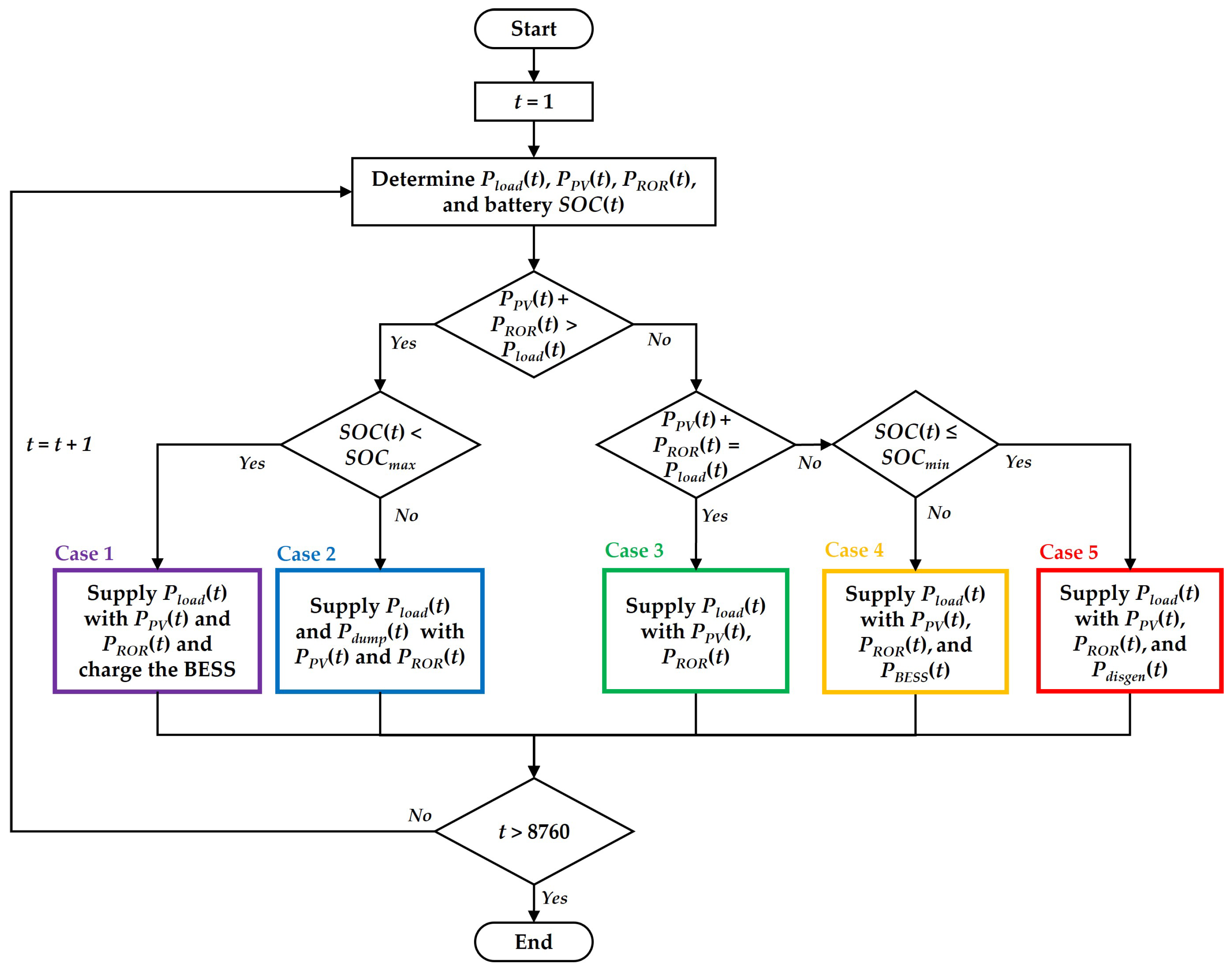
With renewable energy resources being intermittent, a sophisticated power management approach must be devised for HREM, which is particularly important when a dependable supply of energy is required to meet the temporal distribution of load demand. Because the quantity of electricity that can be produced from renewable resources is limited, the capacity of these power generating units cannot be quickly expanded to meet the increasing demand for electricity. As a result, having a power management plan in place would be one of the most important considerations when designing such systems. In order to implement power management strategy in the optimization process, the following cases will be taken into consideration:

Case 1: Energy produced in sufficient quantities is sourced from renewable sources, with any excess energy being utilized to charge a battery bank.

Case 2: This case is similar to Case 1, except that the excess energy produced by renewable resources, PV and ROR hydropower, exceeds the amount of energy required to power the load and the BESS. This means that the excess electricity is used to supply the dump load in this instance.

Case 3: The total power generated by PV and ROR hydropower is just barely sufficient to supply the load demand.

Case 4: The total power generated by PV and ROR hydropower is not enough to meet the load demand of HREM. The utilization of the stored energy in the BESS takes precedence over the operation. The BESS is used to make up for the lack of available power.

Case 5: This case is similar to Case 4, except the SOC of the BESS is at the minimum limit. In this instance, a diesel generator is used to make up for the lack of available power generation.

Figure 7 depicts the primary flowchart for the various modes of operation. In Figure 8 and Figure 9, the algorithms for charging and discharging are shown.

4. Optimization Setup

This section introduces the proposed approach for the optimal sizing and operation of HREM and discusses the details about the objectives considered for the optimization of HREM, constraints of the optimization, decision variables, PSO, and MOPSO.

4.1. Optimization Objectives

The optimization problem is based on minimizing the levelized cost of electricity (LCOE), loss of power supply probability (LPSP), and greenhouse gas (GHG) emissions, simultaneously. Further details about each objective function are discussed in the following subsections.

4.1.1. Levelized Cost of Electricity

The levelized cost of electricity (LCOE) is a well-known and often used metric of a microgrid’s economic feasibility. LCOE is the total cost of installing, operating, and maintaining an HREM in its entirety over the annual energy produced and it also depicts the cost of energy per kWh throughout the system’s lifetime. The annual energy generated and the annual costs are considered to remain constant throughout the lifetime of HREM in this study. A low, levelized cost of energy correlates to a low power cost. The LCOE (USD/kWh) is calculated using the following equation [44,45]:

$$LCOE=\frac{TLC{C}_{HREM}}{E_{ALD}}$$

(10)

$$TLC{C}_{HREM}=TLC{C}_{ROR}+TLC{C}_{PV}+TLC{C}_{BESS}+TLC{C}_{disgen}$$

(11)

$$E_{ALD}=\sum _{t=1}^{8760}{P}_{load}\left(t\right)\times \Delta t$$

(12)

where $TLC{C}_{HREM}$ is the total life cycle cost (TLCC) of HREM (USD); $E_{ALD}$ is annual energy demand of the system (kWh); and $TLC{C}_{ROR}$, $TLC{C}_{PV}$, $TLC{C}_{BESS}$, and $TLC{C}_{disgen}$ are the TLCC of ROR hydropower, PV system, BESS, and diesel generator, respectively.

The TLCC of each component of the HREM is determined based on the component’s capital cost. The $TLC{C}_{ROR}$ and $TLC{C}_{PV}$ are calculated using the following equations [44,45,46]:

$$TLC{C}_{ROR}=P_{ROR}\times C_{cc,ROR}\times \left(1+\frac{C_{om,ROR}}{CRF}\right)$$

(13)

$$TLC{C}_{PV}=N_{PV}\times P_{PV,panel}\times C_{cc,PV}\times \left(1+\frac{C_{om,PV}}{CRF}\right)$$

(14)

$$CRF=\frac{IR·{(1+IR)}^{LT}}{{(1+IR)}^{LT}-1}$$

(15)

where $C_{cc,ROR}$ is the capital cost of ROR (USD/kW); $C_{om,ROR}$ is the operation and maintenance cost of ROR (%/year); $C_{cc,PV}$ is the capital cost of PV (USD/kW); $C_{om,PV}$ is the operation and maintenance cost of PV (%/year); $CRF$ is the capital recovery factor; $IR$ is the interest rate (%); and $LT$ is the lifetime of the system (years).

For BESS, the TLCC is computed using the following equations:

$$TLC{C}_{BESS}=N_{BESS}\times C_{cc,BESS}+\frac{T{E}_{CH,DCH}\times C_{o,BESS}+N_{BESS}\times C_{m,BESS}}{CRF}$$

(16)

$$T{E}_{CH,DCH}=\sum _{t=1}^{8760}(P_{BESS,CH}\left(t\right)+P_{BESS,DCH}\left(t\right))\Delta t$$

(17)

where $C_{cc,BESS}$ is the capital cost of BESS (USD/kWh); $T{E}_{CH,DCH}$ is the total annual energy charged and discharged by the BESS (kWh); $C_{o,BESS}$ is the operation cost (USD/kWh); and $C_{m,BESS}$ is the maintenance cost (USD/kWh).

The TLCC of the diesel generator is determined using the following equations:

$$TLC{C}_{disgen}=N_{disgen}\times C_{cc,dsg}+\frac{n_{dsgh}\times C_{m,dsg}+AF{G}_{disgen}\times C_{o,dsg}}{CRF}$$

(18)

$$AF{C}_{disgen}=\sum _{t=1}^{8760}F{C}_{disgen}\left(t\right)$$

(19)

where $C_{cc,dsg}$ is the capital cost of diesel generator (USD/kW); $n_{dsgh}$ is the total number of operating hours of the diesel generator (h); $C_{m,dsg}$ is the maintenance cost (USD/h); $AF{C}_{disgen}$ is the total annual fuel consumption; and $C_{o,dsg}$ is the operation cost (USD/L).

4.1.2. Loss of Power Supply Probability

Loss of power supply probability (LPSP) is a statistical measure that shows the likelihood of a power supply failure owing to a lack of power generated by renewable energy sources and other power generating components or a breakdown in technical infrastructure to satisfy load demand. It is determined by the following equations:

$$LPSP=\frac{{\sum }_{t=1}^{8760}(P_{load}\left(t\right)+P_{BESS,CH}\left(t\right)-P_{supply}\left(t\right)-P_{BESS,CH}\left(t\right))}{{\sum }_{t=1}^{8760}{P}_{load}\left(t\right)}$$

(20)

$$P_{supply}\left(t\right)=P_{ROR}\left(t\right)+P_{PV}\left(t\right)+P_{disgen}\left(t\right)+P_{BESS,DCH}\left(t\right)$$

(21)

The reliability assessment is carried out under the most adverse situations possible, such as when

$$P_{load}\left(t\right)>P_{supply}\left(t\right)$$

(22)

4.1.3. Greenhouse Gas Emissions

One of the measures for determining the environmental impact of an HREM is the amount of the greenhouse gases (GHG) emitted by its power generating components. HREMs are capable of exploiting the advantages of renewable energy sources and energy storage equipment flexibly and efficiently, and thus having less environmental impact by meeting energy conservation and emission reduction targets. In this study, the amount of GHG produced (kg) by the diesel generator component of HREM is computed using the following equation:

$$GH{G}_{em}=\sum _{t=1}^{8760}F{C}_{disgen}\left(t\right)\times E{F}_{GHG}$$

(23)

$$E{F}_{GHG}=E{F}_{C{O}_2}+E{F}_{C{H}_4}+E{F}_{N_{2}O}+E{F}_{NOx}+E{F}_{CO}$$

(24)

where $E{F}_{GHG}$ is the total emission factor of diesel generator for greenhouse gasses (kg/L) and $E{F}_{C{O}_2}$, $E{F}_{C{H}_4}$, $E{F}_{N_{2}O}$, $E{F}_{NOx}$, and $E{F}_{CO}$ are the carbon dioxide, methane, nitrous oxide, nitrogen oxides, and carbon monoxide emission factors (kg/L), respectively.

4.2. Decision Variables

The HREM’s decision variables may be classified as design variables or operational variables. The independent choice factors for sizing the essential components are as follows: number of the PV panels ($N_{PV}$) which directly determines the size of PV system, diesel generator size ($N_{disgen}$), and size of the BESS ($N_{BESS}$). All of these component sizes influence fuel consumption and greenhouse gas emission, influencing the environmental impact and cost of the system. Getting the optimal size of BESS and diesel generator is beneficial as it improves the flexibility and reliability of the HREM. These decisions variables are continuous variables that are constrained to be real numbers.

The decision variables involved in the HREM are as follows:

$$\overrightarrow{X}={[N_{PV},N_{BESS},N_{disgen}]}^T$$

(25)

4.3. Optimization Constraints

In microgrid optimization research, the constraints on different optimization options are varied. A microgrid’s design and operation should be flexible in order to increase the reliability of a distribution system. Microgrid optimization research is often intimately related to cost optimization, either economically or environmentally. Microgrid power balance, generating capacity, and energy storage are just a few things to consider when determining how well a microgrid should work at all times.

The load–generation balance constraint is defined by the following equation:

$$P_{load}\left(t\right)+P_{BESS,CH}\left(t\right)+P_{dump}\left(t\right)=P_{ROR}\left(t\right)+P_{PV}\left(t\right)+P_{disgen}\left(t\right)+P_{BESS,DCH}\left(t\right)$$

(26)

Each unit, including power producing and energy storage units, has a lower and higher limit on the amount of power or energy it can generate. The following equations describe these constraints:

$$P_{ROR,min}\le P_{ROR}\left(t\right)\le P_{ROR,max}$$

(27)

$$P_{PV,min}\le P_{PV}\left(t\right)\le P_{PV,max}$$

(28)

$$P_{disgen,min}\le P_{disgen}\left(t\right)\le P_{disgen,max}$$

(29)

$$E_{BESS,min}\le E_{BESS}\left(t\right)\le E_{BESS,max}$$

(30)

Limitations on the charging and discharging rates of the storage unit are shown as follows [47,48]:

$$u_{CH}\left(t\right)+u_{DCH}\left(t\right)\le 1$$

(31)

$$SO{C}_{min}\le SOC\left(t\right)\le SO{C}_{max}$$

(32)

$$SOC\left(t\right)=SOC(t-1)+\frac{E_{BESS,CH}\left(t\right)\times u_{CH}\left(t\right)-E_{BESS,DCH}\left(t\right)\times u_{DCH}\left(t\right)}{N_{BESS}}$$

(33)

where $u_{CH}\left(t\right)$ and $u_{DCH}\left(t\right)$ are the charging and discharging states, respectively, with values either 0 or 1, and $SOC\left(t\right)$ and $SOC(t-1)$ are the state of charge of the BESS at the current and previous times, respectively.

4.4. Multi-Objective Optimization

Many real-world problems require simultaneous optimization of multiple objective functions, which are frequently non-proportional and in conflict. This optimization technique produces a collection of solutions rather than an ideal solution, since no one solution can be identified by evaluating all of the objectives at the same time. As a result, the multi-objective optimization (MOO) problem necessitates the simultaneous maximization or minimization of many objective functions while simultaneously satisfying a range of equality and inequality constraints. When a MOO problem has conflicting objectives, it is critical to develop a Pareto front of feasible solutions. Figure 10 shows a sample Pareto front solution set. Non-dominated solutions to optimization problems, such as a Pareto front, disclose actual tradeoffs between various objectives. A non-dominated solution is one in which no other solution performs better on any objective than the non-dominated solution. Due to PSO’s capacity to create a large number of solutions, it excels in multi-objective optimization problems.

Mathematically, multi-objective optimization can be expressed as follows:

$$MinimizeF\left(\overrightarrow{X}\right)={\left[F_1\left(\overrightarrow{X}\right),F_2\left(\overrightarrow{X}\right),\dots ,F_N\left(\overrightarrow{X}\right)\right]}^T$$

(34)

Subject to the following:

$$G_i\left(\overrightarrow{X}\right)<0i=1,2,\dots ,N_{\mathrm{INEQ}}$$

(35)

$$H_i\left(\overrightarrow{X}\right)=0i=1,2,\dots ,N_{\mathrm{EQ}}$$

(36)

where F is a vector comprising the MOO functions; $\overrightarrow{X}$ is a vector containing the decision variables of $F_i\left(\overrightarrow{X}\right)$, representing the ith objective function; $G_i\left(\overrightarrow{X}\right)$ is the inequality constraints; $H_i\left(\overrightarrow{X}\right)$ is the equality constraints; and N is the number of objective functions defined in the problem.

Two conditions must be satisfied in order to decide if one solution dominates the other. First, the solution must be no worse than the others in all of the objective functions. Second, the solution is objectively superior than the alternative in all respects. It can be described as follows:

$$F_j\left(X_1\right)\le F_k\left(X_2\right)\exists k\in \left\{1,2,\dots ,N\right\}$$

(37)

$$F_k\left(X_1\right)\le F_j\left(X_2\right)\forall j\in \left\{1,2,\dots ,N\right\}$$

(38)

4.5. Particle Swarm Optimization

Particle swarm optimization (PSO), which Kennedy and Eberhart initially defined in 1995, is driven by two distinct concepts: swarm intelligence, which is based on the social interaction of swarms, and evolutionary computing [49]. In the PSO algorithm, the best two values determine the position of every particle. The first value is the particle’s current maximum value, which has been kept and is also known as the particle’s “personal best”. The second value is termed the “global best”, which is generated by the algorithm from the population’s current state. Additionally, every particle has a position, which indicates the values of the variables, and a velocity that drives it toward personal and global bests. The fitness function is an objective function that determines the optimal solution from among all feasible solutions. Constraints may also be applied to the fitness function of PSO. The PSO method is shown in Figure 11.

While the algorithm is being executed, each particle retains the best fitness value that it obtained throughout the course of the process. Furthermore, the particle with the best fitness value in contrast to the rest of the particles is determined and updated during the iteration process. When certain stopping criteria are met, such as the maximum number of iterations or the defined objective fitness values, the algorithm terminates. When a particle in the swarm moves, the position of that particle is updated using the following equation:

$$x_i(k+1)=x_i\left(k\right)+v_i(k+1)$$

(39)

where x is particle position and v is particle velocity in the iteration k. The velocity is calculated as follows:

$$v_i(k+1)=K\times v_i\left(k\right)+C_1{R}_1\left(P_{i,best}\left(k\right)-x_i\left(k\right)\right)+C_2{R}_2\left(G_{best}\left(k\right)-x_i\left(k\right)\right)$$

(40)

$$K=\frac{2}{2-\phi -\sqrt{{\phi }^2-4\phi }}$$

(41)

$$\phi =C_1-C_2\phi >4$$

(42)

where $P_{i,best}$ is ith particle’s personal best position; $G_{best}$ is the global best position of the entire population; $C_1$ is the cognitive acceleration coefficient; $C_2$ is the social acceleration coefficient; and $R_1$ and $R_2$ are randomly generated numbers ranging from 0 to 1.

The equation for calculating the velocity of the particle contains two components. The first component, known as the cognitive component ($C_1{R}_1\left(P_{i,best}\left(k\right)-x_i\left(k\right)\right)$), influences the particle to return to a previous position where it had a higher personal fitness value, whereas the second component, known as the social component ($C_2{R}_2\left(G_{best}\left(k\right)-x_i\left(k\right)\right)$), directs it to the best area that the swarm or population has located thus far and to follow the direction of the best neighbor.

4.6. Application of MOPSO to HREM Optimization

The multiple objective functions ($LCOE$, $LPSP$, and $GH{G}_{em}$) are solved in this work using the MOPSO algorithm, which is based on the PSO algorithm. PSO is recognized for having fast convergence, and although this is desirable in the optimization process, it may result in a false Pareto solution in MOPSO. As a result, MOPSO introduces a mutation operator, which is used after the particle’s position is changed and thereby alters the position vector [50]

Compared with other existing algorithms that are also capable of solving MOO problems, MOPSO has relatively fewer parameters that need to be tuned, and it uses a fast convergent search operator to achieve its speed. The algorithm can also be easily modified to improve its performance, and it can achieve sub-optimal and optimal solutions in a relatively shorter amount of computational time than most other algorithms [51,52]. The MOPSO algorithm shown in Figure 12 can be readily applied to our problem according to the following steps.

Step 1 The first step is to gather input data for the optimization. To begin, primary data includes information on the structure of the sample HREM, the technical and functional characteristics of the inverter, BESS, diesel generator, run-of-river hydropower, and solar power estimates for the next 24 hours, climatic conditions, and the daily load curve.

Step 2 Initialize the optimization process by generating the initial population, while taking into account the constraints of the problem, including the minimum and maximum values of decision variables.

Step 3 The created initial population is subjected to the load–generation balance, the proposed power management strategy, and other constraints.

All of these constraints are applied to each population formed, and the corresponding fitness function values are determined.

Step 4 Based on the generated solutions, determine non-dominated solutions.

Step 5 After identifying the solutions that are non-dominated, separate them from the dominated solutions and store them in an archive.

Step 6 The best particle is picked as a leader after storing the non-dominated solutions.

Step 7 Using Equations (39) and (40), calculate the updated position and velocity of each particle.

Step 8 Update each particle’s best position after calculating their updated velocity and position.

Step 9 Remove non-dominated members from the archive after updating each particle’s best position.

Step 10 Examine the terminating conditions; if favorable optimal conditions for the optimization process are attained, the algorithm is halted; otherwise, the procedure is resumed from Step 6.

Step 11 After finding the best Pareto solution from the non-dominated solutions, selecting a better option from the ideal solution is deemed required and critical for microgrid design and operation.

5. Results and Discussions

5.1. Initialization

To set up the optimization of HREM, several parameters were set and initialized.

Table 2. HREM financial parameters.

Parameter	Variable	Value	Unit
Discount rate	$IR$	6	%
System life time	$LT$	20	years

shows the HREM’s overall financial parameters while

Table 3. HREM component model and manufacturer.

Component	Model	Manufacturer
PV	YL250P-29b Solar Panels	Yingli Solar
ROR Hydropower	Barrel Turbine Generating Unit	Hangzhou Regional Center (HRC)
Diesel Generator	DE33 GC Genset	CAT
BESS	352V1200AH	Jingsun Battery

shows the component model and manufacturer.

Table 4. HREM component financial and technical parameters.

Component	Parameter	Variable	Value	Unit
ROR Hydropower	Design Flow	$Q_D$	0.12	m${}^3$/s
	Gross Head	$H_G$	12	meters
	Penstock length	L	100	meters
	Pipe Diameter	D	0.25	meters
	Hazen–Williams Coefficient	C	200
	Turbine Efficiency	${\eta }_t$	85	%
	Generator Efficiency	${\eta }_g$	93	%
	Capital Cost	$C_{cc,ROR}$	3400	USD/kW
	Operation and Maintenance Cost	$C_{om,ROR}$	4	% initial inv./year
PV System	Panel Rating	$P_{PV,rating}$	0.25	kilowatts
	Temperature Coefficient of PV	${\gamma }_{pv}$	−0.3	%${/}^{\circ }$ Celsius
	PV Regulator Efficiency	${\eta }_R$	95	%
	Nominal Operation Cell Temperature	$NOCT$	41.5	${}^{\circ }$C
	Reference Temperature	$T_{REF}$	25	${}^{\circ }$C
	Capital Cost	$C_{cc,PV}$	1722.3	USD/kW
	Operation and Maintenance Cost	$C_{om,PV}$	1	% initial inv./year
BESS	Minimum State of Charge	$SO{C}_{min}$	20	%
	Minimum State of Charge	$SO{C}_{max}$	90	%
	Charging Efficiency	${\eta }_{BESS,CH}$	80	%
	Discharging Efficiency	${\eta }_{BESS,DCH}$	100	%
	Capital Cost	$C_{cc,BESS}$	241.31	USD/kW
	Operation Cost	$C_{o,BESS}$	0.00045	USD/kWh
	Maintenance Cost	$C_{m,BESS}$	11.10	USD/kWh-year
Diesel Generator	Carbon Dioxide Emission Factor	$E{F}_{C{O}_2}$	2.7	kg/L
	Methane Emission Factor	$E{F}_{C{H}_4}$	$5.1\times {10}^{-5}$	kg/L
	Nitrous Oxide Emission Factor	$E{F}_{N_{2}O}$	$1.7\times {10}^{-4}$	kg/L
	Nitrogen Oxides Emission Factor	$E{F}_{NOx}$	$1.36\times {10}^{-2}$	kg/L
	Carbon Monoxide Emission Factor	$E{F}_{CO}$	$1.53\times {10}^{-2}$	kg/L
	Fixed Consumption Coefficient	${\alpha }_{DSG}$	0.3058	L/kWh
	Variable Consumption Coefficient	${\beta }_{DSG}$	0.0206	L/kWh
	Capital Cost	$C_{cc,dsg}$	377.26	USD/kW
	Operation Cost	$C_{o,dsg}$	1.61	USD/L
	Maintenance Cost	$C_{m,dsg}$	1.13	USD/L

shows the technical and financial parameters used for each components. For the optimization process,

Table 5. MOPSO parameters.

Parameter	Value	Parameter	Value
Population Size	100	w	0.4
Max Iteration	100	$C_1$	2
$N_{archive}$	200	$C_2$	2
Mutation percentage	0.5	$N_{grid}$	20
$v_{max}$	5

shows the values of the parameters used. The minimum and maximum values of the decision variables are also shown in

Table 6. Minimum and maximum values of decision variables.

Decision Variable	Min. Value	Max. Value
$N_{disgen}$	0	30 kW
$N_{BESS}$	0	100 kWh
$N_{PV}$	0	100 panels

. The values of technical and economic parameters were either calculated and estimated based on the geographical conditions of the study area or taken from several sources which include product data sheet, previously published studies, reports, and manuals on diesel generators, PV, BESS, and ROR hydropower design [44,46,53,54,55,56,57,58,59,60].

5.2. Optimization Results

The Pareto optimal solution set was acquired by running the multi-objective optimization algorithm program. Figure 13 and Figure 14 show the 3D and 2D Pareto front results of the optimization, respectively. As shown in Figure 13, the value of each coordinate axis represents the objective functions while the non-dominated solutions obtained from the optimization form the Pareto front. In Figure 14, it can be seen that the lower the LPSP of a solution, the higher its LCOE and GHG emissions. Solutions with diesel generator components have lower LPSP values and higher LCOE and GHG emission values. The optimization generated values of LCOE, LPSP, and GHG emissions, varying in the ranges 0.0446–0.2556 USD/kWh, 0.0001–0.3201, and 0–16,598 kg, respectively. To simplify the analysis of the Pareto front formed by the non-dominated solutions, A, B, C, and D are located and chosen as solutions of interest. The solutions enclosed in the blue dashed line, which include solutions A and B, are the non-dominated solutions generated by the algorithm without a diesel generator component, while the non-dominated solutions that are enclosed by the purple dashed line, which include solutions C and D, are non-dominated solutions with a diesel generator component. Solutions A and B showed least value of LCOE and LPSP, respectively, while D contains the least LPSP overall. Solution C, which is midway between B and D, has the tradeoff of increasing the GHG emissions and LCOE. However, this tradeoff also decreased the LPSP, which ensures greater reliability for the HREM. Thus, C was chosen for further analysis of the operation of HREM.

Table 7. Optimization solutions of interest.

Solution	${\mathit{N}}_{\mathit{disgen}}$	${\mathit{N}}_{\mathit{batt}}$	${\mathit{N}}_{\mathit{PV}}$	$\mathit{LCOE}$	$\mathit{LPSP}$	${\mathit{GHG}}_{\mathit{em}}$
	(kW)	(kWh)	No. of Panels	(USD/kWh)	(%)	(kg)
A	0	0	0	0.0446	32	0
B	0	100	100	0.1245	2.74	0
C	13	100	100	0.1795	0.51	7874
D	20	100	100	0.2027	0	12,748

shows the values of the objective functions and decision variables for solutions of interest. On an AMD Ryzen 7 3700U @ 2.30 GHz, 8 GB RAM system, the developed programs are run using MATLAB software.

5.3. Monthly Energy Output

The monthly electricity generation by the system for four different solutions, A–D, is shown in Figure 15, Figure 16, Figure 17 and Figure 18, respectively. As shown in Figure 15, Solution A, with decision variable values of $N_{disgen}$ = 0, $N_{batt}$ = 0, and $N_{PV}$ = 0, only has the hydropower as generation component producing varied monthly energy from 6720 kWh (lowest) to 7440 kWh (highest). The energy produced by hydropower alone is not enough to supply the monthly energy demand. Thus, this solution is not feasible for the reliable operation of HREM. Although Solution A has the lowest LCOE of 0.0446 USD/kWh and zero GHG emissions due to the absence of a diesel generator component, it has the highest LPSP of 32%, which means the system’s operation is highly unreliable. On the other hand, Solution B, with decision variable values of $N_{disgen}$ = 0, $N_{batt}$ = 100 kWh, and $N_{PV}$ = 100 panels, has an LCOE of 0.1245 USD/kWh with an LPSP of 2.74% and zero GHG emissions. It is the solution with the lowest LPSP within the Pareto front that has zero GHG emissions. As shown in Figure 16, the energy produced by hydropower is the same in Solution A with a monthly PV energy output varying from 2450 kWh (lowest) to 4111 kWh (highest), while the monthly BESS energy discharge varies from 1379 kWh (lowest) to 2264 kWH (highest).

Solutions C and D have the same monthly hydropower energy output as Solution A. However, both of these solutions have diesel generator components. Solution C, with $N_{disgen}$ = 13 kW, $N_{batt}$ = 100 kWh, and $N_{PV}$ = 100 panels, has an LCOE of 0.1795 USD/kWh, LPSP of 0.51%, and GHG emission of 7874 kg; meanwhile, Solution D, with $N_{disgen}$ = 20 kW, $N_{batt}$ = 100 kWh, and $N_{PV}$ = 100 panels, has an LCOE of 0.2027 USD/kWh, LPSP of 0%, and GHG emission of 12,748 kg. The monthly energy output from the diesel generator varies from 435 kWH to 759 kWh for Solution C and from 717 kWh to 1045 kWh for Solution D. As shown in Figure 17 and Figure 18, the diesel generator only has a monthly energy output in the months of May, June, September, and December. In these months, the diesel generator operates due to increased load from agricultural activities.

5.4. Energy Scheduling Analysis

To determine the performance of the system, four scenarios were considered for the scheduling analysis using component sizes from Solution C, shown in

Table 8. Four scenarios for HREM scheduling analysis.

Scenario	Condition
1	No Agricultural Load and Low Solar Radiation
2	No Agricultural Load and High Solar Radiation
3	With Agricultural Load and Low Solar Radiation
4	With Agricultural Load and High Solar Radiation

. The scenarios determine how the HREM performs under varying meteorological and load conditions. Figure 19, Figure 20, Figure 21 and Figure 22 show the results of the energy scheduling based on different conditions.

For Scenarios 1 and 2, shown in Figure 19 and Figure 20, respectively, the HREM operates with surplus power and the diesel generator is not being dispatched. This is due to the power generated by renewable energies being more than enough for the load from morning to afternoon. In the evening, when the load peaks, the battery dispatches the energy stored in the BESS from the charged excess energy. It can also be seen that, in both scenarios, the SOC of the battery varies from 20% to 90%. Thus, the constraints imposed on the battery’s SOC are not violated.

In Scenario 3, there is an agricultural load from Monday to Saturday, and there are certain days with low solar radiation. As shown in Figure 21, the power generated by PV and hydropower is not enough to supply the combined residential and agricultural load and charge the battery with a surplus. The BESS discharges in both the morning and evening, unlike in Scenario 1 and 2. This is due to high load demand from 7 a.m. to 10 a.m. and from 7 p.m. to 10 p.m. It can also be seen in the figure that the diesel generator is being dispatched in the evening, when the load is at its peak, to compensate for the insufficient power generated by the hydropower and battery. There are days in this scenario where the SOC does not reach its maximum value of 90% and often dips below 30%.

As shown in Figure 22, in the scenario where there is high solar radiation, the power generated by each component of HREM is just enough for the combined residential and agricultural load and charging BESS. Thus, there is a small to zero surplus of power for the dump load except on Sunday when the load is only residential. The diesel generator operates sometimes for an hour when the load is at its peak. In the evening, the load peaks and the power generated by hydropower alone is insufficient, so the BESS starts discharging power to compensate. Except for Sunday, the SOC of the battery in this scenario often dips below 30% due to increased load and less excess energy from renewables for charging, as compared with Scenarios 1 and 2.

5.5. Sensitivity Analysis

The sensitivity analysis was expanded to qualify and quantify the influence of parametric variation on the levelized cost of electricity for HREM, as computed using the MOPSO algorithm. As sensitivity coefficients, four input parameters were chosen, and the results were determined with regard to Solution C, which is one of the solutions of interest and the nominal point in Table 7. Due to variations in the number of PV panels, size of diesel generator, size of BESS, and rural agricultural load of the study area, the influence on LCOE, as one of the main objectives, was investigated. Parameter variations from 50% to 150% were evaluated for sensitivity analysis and the sensitivity curve is shown in Figure 23. The LCOE is affected by the rural agriculture load, PV, and BESS in a nonlinear way. Because the total annual energy demand for the system is lower when the load is reduced, the LCOE values are higher. The LCOE is also influenced by a variation in the size of the diesel generator due to capital cost and fuel consumption, as seen in the graph. It can be seen that, with a lower rural agricultural load, number of PV panels, and BESS size, the LCOE values are higher and more sensitive. The LCOE is least affected by the number of PV panels. The reason for this is that the PV system has a lower overall cost (capital, operating, and maintenance) as compared with other components of the system.

6. Conclusions

This study presents the optimal design of an off-grid hybrid renewable energy microgrid system that can be used in order to meet the electrical load requirements in selected rural agricultural communities in the Southern Philippines. The multi-objective particle swarm optimization (MOPSO) algorithm is used to find the optimal system design and component sizes. The levelized cost of electricity (COE), the probability of loss of power supply (LPSP), and greenhouse gas emissions are all objective functions. A sensitivity analysis was also carried out to find out how much a change in the input values for a certain variable affects the results of the mathematical models that were used.

The algorithm generated 200 non-dominated solutions, of which 4 were selected as solutions of interest. Based on the results, the optimal size of the main components for the reliable operation of the system was estimated for the PV as 200 panels with a rating of 0.25 kW, for BESS as 100 kWh, and for the diesel generator as 13 kW, with an estimated system LCOE, LPSP, and GHG emission of 0.197 USD/kWh, 0.05%, and 7874 kg, respectively, for 1 year. The amount of energy generated by each component in a month using the HREM configuration that has been chosen is more than adequate to meet the rural agriculture load and the dump load. The sensitivity analysis showed that decreased rural agricultural demand, PV panel count, and BESS size result in higher LCOE values, and that LCOE is least impacted by PV panel count, respectively. Furthermore, the main achievements and conclusions are listed below:

• An optimized design of a hybrid renewable energy microgrid (HREM) composed of ROR hydropower, PV, BESS, and a diesel generator to supply electricity considering cost, reliability, and environmental impact.
• A framework for simultaneous optimization of multiple generating units considering renewable energy’s intermittent nature using MOPSO with three conflicting objectives, which are LCOE, LPSP, and GHG emissions, several constraints, and real meteorological data.
• The proposed method also determines the capacity of each component of the system while considering the availability of renewable energy sources, load size, and several cost functions in order to obtain the configuration, while considering different tradeoffs for the lifetime of the microgrid in order to minimize costs and maximize reliability.
• A power management strategy for optimal operation of the various components of the system and to ensure effective charging and discharging of the battery.
• Energy demand estimation for an unelectrified rural agricultural area and load profiles for residential and agricultural loads were used for the optimization of the HREM.
• Investigation and evaluation of the performance of the optimal design of HREM considering several scenarios within the study area.

In future work, investigating and developing techniques for handling other uncertainty factors in the design and optimization of HREMs, as well as microgrid stability, might prove important. This work’s important findings and contributions can be used for future studies in the area of developing deep learning or artificial neural network algorithms for a more flexible solution to the optimization issue. Furthermore, more research into techniques to enhance the reliable and economically justifiable use of diverse renewable energy sources in microgrids and power systems could also be the focus of future studies. More study is required to find the most effective strategy to employ excess RE in off-grid HREMs. Furthermore, the study results will be valuable in the management of renewable energy resources, planning and development, and rural electrification.

References

1. IEA. IEA—World Energy Outlook 2019. Available online: https://www.iea.org/reports/world-energy-outlook-2019 (accessed on 15 August 2021).
2. The World Bank. World Bank—Report: Universal Access to Sustainable Energy Will Remain Elusive without Addressing Inequalities. Available online: https://www.worldbank.org/en/news/press-release/2021/06/07/report-universal-access-to-sustainable-energy-will-remain-elusive-without-addressing-inequalities (accessed on 7 August 2021).
3. Jasiński, J.; Kozakiewicz, M.; Sołtysik, M. Determinants of Energy Cooperatives’ Development in Rural Areas—Evidence from Poland. Energies 2021, 14, 319. [Google Scholar] [CrossRef]
4. Quirapas-Franco, M.A. Sustainable Energy Transition of the Poor Rural Communities in the Philippines. 2021. Available online: https://www.stratforumph.com/post/sustainable-energy-transition-of-the-poor-rural-communities-in-the-philippines (accessed on 22 August 2021).
5. Ton, D.T.; Smith, M.A. The U.S. Department of Energy’s Microgrid Initiative. Electr. J. 2012, 25, 84–94. [Google Scholar] [CrossRef]
6. Rehmani, M.H.; Reisslein, M.; Rachedi, A.; Erol-Kantarci, M.; Radenkovic, M. Integrating Renewable Energy Resources Into the Smart Grid: Recent Developments in Information and Communication Technologies. IEEE Trans. Ind. Inform. 2018, 14, 2814–2825. [Google Scholar] [CrossRef]
7. Swain, P.; Jagadish, S.; Uma Mahesh, K.N.S. Integration of renewable sources of energy into power grid. In Proceedings of the 2017 IEEE Region 10 Symposium (TENSYMP), Cochin, India, 14–16 July 2017; pp. 1–5. [Google Scholar] [CrossRef]
8. An, L.N.; Tuan, T.Q. Dynamic Programming for Optimal Energy Management of Hybrid Wind–PV–Diesel–Battery. Energies 2018, 11, 3039. [Google Scholar] [CrossRef] [Green Version]
9. Nguyen, M.Y.; Yoon, Y.T.; Choi, N.H. Dynamic programming formulation of Micro-Grid operation with heat and electricity constraints. In Proceedings of the 2009 Transmission Distribution Conference Exposition: Asia and Pacific, Seoul, Korea, 26–30 October 2009; pp. 1–4. [Google Scholar] [CrossRef]
10. Střelec, M.; Berka, J. Microgrid energy management based on approximate dynamic programming. In Proceedings of the IEEE PES ISGT Europe 2013, Lyngby, Denmark, 6–9 October 2013; pp. 1–5. [Google Scholar] [CrossRef]
11. Gan, L.K.; Shek, J.K.; Mueller, M.A. Hybrid wind–photovoltaic–diesel–battery system sizing tool development using empirical approach, life-cycle cost and performance analysis: A case study in Scotland. Energy Convers. Manag. 2015, 106, 479–494. [Google Scholar] [CrossRef] [Green Version]
12. Yoldas, Y.; Goren, S.; Onen, A. Optimal Control of Microgrids with Multi-stage Mixed-integer Nonlinear Programming Guided Q-learning Algorithm. J. Mod. Power Syst. Clean Energy 2020, 8, 1151–1159. [Google Scholar] [CrossRef]
13. Batiyah, S.; Sharma, R.; Abdelwahed, S.; Zohrabi, N. An MPC-based power management of standalone DC microgrid with energy storage. Int. J. Electr. Power Energy Syst. 2020, 120, 105949. [Google Scholar] [CrossRef]
14. Fouladi, E.; Baghaee, H.R.; Bagheri, M.; Gharehpetian, G.B. Power Management of Microgrids Including PHEVs Based on Maximum Employment of Renewable Energy Resources. IEEE Trans. Ind. Appl. 2020, 56, 5299–5307. [Google Scholar] [CrossRef]
15. Oulis Rousis, A.; Tzelepis, D.; Konstantelos, I.; Booth, C.; Strbac, G. Design of a Hybrid AC/DC Microgrid Using HOMER Pro: Case Study on an Islanded Residential Application. Inventions 2018, 3, 55. [Google Scholar] [CrossRef] [Green Version]
16. Aziz, A.S.; Tajuddin, M.F.N.; Adzman, M.R.; Ramli, M.A.M.; Mekhilef, S. Energy Management and Optimization of a PV/Diesel/Battery Hybrid Energy System Using a Combined Dispatch Strategy. Sustainability 2019, 11, 683. [Google Scholar] [CrossRef] [Green Version]
17. Lu, J.; Wang, W.; Zhang, Y.; Cheng, S. Multi-Objective Optimal Design of Stand-Alone Hybrid Energy System Using Entropy Weight Method Based on HOMER. Energies 2017, 10, 1664. [Google Scholar] [CrossRef] [Green Version]
18. Oladigbolu, J.O.; Ramli, M.A.M.; Al-Turki, Y.A. Optimal Design of a Hybrid PV Solar/Micro-Hydro/Diesel/Battery Energy System for a Remote Rural Village under Tropical Climate Conditions. Electronics 2020, 9, 1491. [Google Scholar] [CrossRef]
19. García-Vera, Y.E.; Dufo-López, R.; Bernal-Agustín, J.L. Techno-Economic Feasibility Analysis through Optimization Strategies and Load Shifting in Isolated Hybrid Microgrids with Renewable Energy for the Non-Interconnected Zone (NIZ) of Colombia. Energies 2020, 13, 6146. [Google Scholar] [CrossRef]
20. Chae, W.K.; Lee, H.J.; Won, J.N.; Park, J.S.; Kim, J.E. Design and Field Tests of an Inverted Based Remote MicroGrid on a Korean Island. Energies 2015, 8, 8193–8210. [Google Scholar] [CrossRef]
21. Cardoso, G.; Brouhard, T.; DeForest, N.; Wang, D.; Heleno, M.; Kotzur, L. Battery aging in multi-energy microgrid design using mixed integer linear programming. Appl. Energy 2018, 231, 1059–1069. [Google Scholar] [CrossRef]
22. Park, W.H.; Abunima, H.; Glick, M.B.; Kim, Y.S. Energy Curtailment Scheduling MILP Formulation for an Islanded Microgrid with High Penetration of Renewable Energy. Energies 2021, 14, 6038. [Google Scholar] [CrossRef]
23. Krishnan Prakash, A.; Zhang, K.; Gupta, P.; Blum, D.; Marshall, M.; Fierro, G.; Alstone, P.; Zoellick, J.; Brown, R.; Pritoni, M. Solar+ Optimizer: A Model Predictive Control Optimization Platform for Grid Responsive Building Microgrids. Energies 2020, 13, 3093. [Google Scholar] [CrossRef]
24. Balderrama, S.; Lombardi, F.; Riva, F.; Canedo, W.; Colombo, E.; Quoilin, S. A two-stage linear programming optimization framework for isolated hybrid microgrids in a rural context: The case study of the “El Espino” community. Energy 2019, 188, 116073. [Google Scholar] [CrossRef]
25. Yousif, M.; Ai, Q.; Gao, Y.; Wattoo, W.A.; Jiang, Z.; Hao, R. Application of Particle Swarm Optimization to a Scheduling Strategy for Microgrids Coupled with Natural Gas Networks. Energies 2018, 11, 3499. [Google Scholar] [CrossRef] [Green Version]
26. Sun, Y.; Cai, Z.; Zhang, Z.; Guo, C.; Ma, G.; Han, Y. Coordinated Energy Scheduling of a Distributed Multi-Microgrid System Based on Multi-Agent Decisions. Energies 2020, 13, 4077. [Google Scholar] [CrossRef]
27. Torres-Madroñero, J.L.; Nieto-Londoño, C.; Sierra-Pérez, J. Hybrid Energy Systems Sizing for the Colombian Context: A Genetic Algorithm and Particle Swarm Optimization Approach. Energies 2020, 13, 5648. [Google Scholar] [CrossRef]
28. Wu, X.; Cao, W.; Wang, D.; Ding, M. A Multi-Objective Optimization Dispatch Method for Microgrid Energy Management Considering the Power Loss of Converters. Energies 2019, 12, 2160. [Google Scholar] [CrossRef] [Green Version]
29. Khlifi, F.; Cherif, H.; Belhadj, J. Environmental and Economic Optimization and Sizing of a Micro-Grid with Battery Storage for an Industrial Application. Energies 2021, 14, 5913. [Google Scholar] [CrossRef]
30. Dufo-López, R.; Bernal-Agustín, J.L.; Yusta-Loyo, J.M.; Domínguez-Navarro, J.A.; Ramírez-Rosado, I.J.; Lujano, J.; Aso, I. Multi-objective optimization minimizing cost and life cycle emissions of stand-alone PV–wind–diesel systems with batteries storage. Appl. Energy 2011, 88, 4033–4041. [Google Scholar] [CrossRef]
31. Vasanth, J.D.; Kumarappan, N.; Arulraj, R.; Vigneysh, T. Minimization of operation cost of a microgrid using firefly algorithm. In Proceedings of the 2017 IEEE International Conference on Intelligent Techniques in Control, Optimization and Signal Processing (INCOS), Srivilliputtur, India, 23–25 March 2017; pp. 1–6. [Google Scholar] [CrossRef]
32. Colson, C.; Nehrir, M.; Wang, C. Ant colony optimization for microgrid multi-objective power management. In Proceedings of the 2009 IEEE/PES Power Systems Conference and Exposition, Seattle, WA, USA, 15–18 March 2009; pp. 1–7. [Google Scholar] [CrossRef]
33. Nimma, K.S.; Al-Falahi, M.D.A.; Nguyen, H.D.; Jayasinghe, S.D.G.; Mahmoud, T.S.; Negnevitsky, M. Grey Wolf Optimization-Based Optimum Energy-Management and Battery-Sizing Method for Grid-Connected Microgrids. Energies 2018, 11, 847. [Google Scholar] [CrossRef] [Green Version]
34. Helmi, A.M.; Carli, R.; Dotoli, M.; Ramadan, H.S. Efficient and Sustainable Reconfiguration of Distribution Networks via Metaheuristic Optimization. IEEE Trans. Autom. Sci. Eng. 2022, 19, 82–98. [Google Scholar] [CrossRef]
35. Muhammad, M.A.; Mokhlis, H.; Naidu, K.; Amin, A.; Franco, J.F.; Othman, M. Distribution Network Planning Enhancement via Network Reconfiguration and DG Integration Using Dataset Approach and Water Cycle Algorithm. J. Mod. Power Syst. Clean Energy 2020, 8, 86–93. [Google Scholar] [CrossRef]
36. PAGASA. PAGASA—Climate of the Philippines. Available online: https://www.pagasa.dost.gov.ph/information/climate-philippines (accessed on 15 August 2021).
37. Badang, D.A.Q.; Sarip, C.F.; Tahud, A.P. Geographic Information System (GIS) and Multicriteria Decision Making (MCDM) for Optimal Selection of Hydropower Location in Rogongon, Iligan City. In Proceedings of the 2018 IEEE 10th International Conference on Humanoid, Nanotechnology, Information Technology, Communication and Control, Environment and Management (HNICEM), Baguio City, Philippines, 29 November–2 December 2018; pp. 1–5. [Google Scholar] [CrossRef]
38. Lorenzo, E. Energy collected and delivered by PV modules. In Handbook of Photovoltaic Science an Engineering; John Wiley & Sons: Hoboken, NJ, USA, 2011. [Google Scholar]
39. Vedel, P. Modeling and Real Time Optimization of a Smart Microgrid. Master’s Thesis, Technical University of Liberec, Liberec, Czech Republic, 2019. [Google Scholar]
40. Jiang, X.; Nan, G.; Liu, H.; Guo, Z.; Zeng, Q.; Jin, Y. Optimization of Battery Energy Storage System Capacity for Wind Farm with Considering Auxiliary Services Compensation. Appl. Sci. 2018, 8, 1957. [Google Scholar] [CrossRef] [Green Version]
41. JICA. Guideline and Manual for Hydropower Development; Open JICA Report; JICA: Tokyo, Japan, 2011; Volume 2.
42. Ismail, M.; Moghavvemi, M.; Mahlia, T. Techno-economic analysis of an optimized photovoltaic and diesel generator hybrid power system for remote houses in a tropical climate. Energy Convers. Manag. 2013, 69, 163–173. [Google Scholar] [CrossRef]
43. Kewat, S.; Singh, B.; Hussain, I. Power management in PV-battery-hydro based standalone microgrid. IET Renew. Power Gener. 2018, 12, 391–398. [Google Scholar] [CrossRef]
44. Short, W.; Packey, D.; Holt, T. A Manual for the Economic Evaluation of Energy Efficiency and Renewable Energy Technologies; NASA STI/Recon Technical Report N; National Renewable Energy Lab. (NREL): Golden, CO, USA, 1995. [Google Scholar] [CrossRef] [Green Version]
45. Phommixay, S.; Doumbia, M.; St-Pierre, D. Review on the cost optimization of microgrids via particle swarm optimization. Int. J. Energy Environ. Eng. 2019, 11, 73–89. [Google Scholar] [CrossRef] [Green Version]
46. Malheiro, A.; Castro, P.M.; Lima, R.M.; Estanqueiro, A. Integrated sizing and scheduling of wind/PV/diesel/battery isolated systems. Renew. Energy 2015, 83, 646–657. [Google Scholar] [CrossRef] [Green Version]
47. Sperstad, I.B.; Korpås, M. Energy Storage Scheduling in Distribution Systems Considering Wind and Photovoltaic Generation Uncertainties. Energies 2019, 12, 1231. [Google Scholar] [CrossRef] [Green Version]
48. Akter, H.; Howlader, H.O.R.; Saber, A.Y.; Hemeida, A.M.; Takahashi, H.; Senjyu, T. Optimal Sizing and Operation of Microgrid in a Small Island Considering Advanced Direct Load Control and Low Carbon Emission. In Proceedings of the 2021 International Conference on Science Contemporary Technologies (ICSCT), Dhaka, Bangladesh, 5–7 August 2021; pp. 1–5. [Google Scholar] [CrossRef]
49. Kennedy, J.; Eberhart, R. Particle swarm optimization. In Proceedings of the ICNN’95—International Conference on Neural Networks, Perth, WA, Australia, 27 November–1 December 1995; Volume 4, pp. 1942–1948. [Google Scholar] [CrossRef]
50. Coello, C.; Pulido, G.; Lechuga, M. Handling multiple objectives with particle swarm optimization. IEEE Trans. Evol. Comput. 2004, 8, 256–279. [Google Scholar] [CrossRef]
51. Yang, X.S. Chapter 8—Particle Swarm Optimization. In Nature-Inspired Optimization Algorithms, 2nd ed.; Yang, X.S., Ed.; Academic Press: Cambridge, MA, USA, 2021; pp. 111–121. [Google Scholar] [CrossRef]
52. Yang, L.; Yang, X.; Wu, Y.; Liu, X. Applied Research on Distributed Generation Optimal Allocation Based on Improved Estimation of Distribution Algorithm. Energies 2018, 11, 2363. [Google Scholar] [CrossRef] [Green Version]
53. Zahboune, H.; Zouggar, S.; Krajacic, G.; Varbanov, P.S.; Elhafyani, M.; Ziani, E. Optimal hybrid renewable energy design in autonomous system using Modified Electric System Cascade Analysis and Homer software. Energy Convers. Manag. 2016, 126, 909–922. [Google Scholar] [CrossRef]
54. IRENA. Renewable Energy Technologies: Cost Analysis Series; IRENA: Abu Dhabi, United Arab Emirates, 2012; Volume 1: Power Sector Issue 3/5, pp. 1–3, 17–25. [Google Scholar]
55. IPCC. 2019 Refinement to the 2006 IPCC Guidelines for National Greenhouse Gas Inventories; The Intergovernmental Panel on Climate Change (IPCC): Geneva, Switzerland, 2019. [Google Scholar]
56. Bhatnagar, D. DOE/EPRI Electricity Storage Handbook; Technical Report; Sandia National Lab. (SNL-NM): Albuquerque, NM, USA, 2012. [Google Scholar]
57. Yingli Solar. YGE 60 Cell Series; Yingli Solar: Baoding, China, 2013; Rev. 1. [Google Scholar]
58. Hangzhou Regional Center (HRC). Barrel Turbine Generating Unit; Hangzhou Regional Center (HRC): Hangzhou, China, 2019. [Google Scholar]
59. Cat. Cat® DE33GC Diesel Generator Sets. 2020. Available online: https://www.cat.com/en_US/products/new/power-systems/electric-power/diesel-generator-sets/107842.html (accessed on 18 September 2021).
60. Jingsun Battery. Rechargeable Lithium Ion Storage Battery. 2019. Available online: https://m.made-in-china.com/product/6000cyles-LiFePO4-100kwh-200kwh-500kwh-1000kwh-Rechargeable-Lithium-Ion-Storage-Battery-886504855.html (accessed on 18 September 2021).
Figure 1. Study area—rural agricultural area composed of five unelectrified sitios, or sites, in Rogongon, Iligan City, Lanao del Norte, Philippines.
Energies 15 02251 g001
Figure 2. Hourly solar radiation in Rogongon, Iligan City.
Energies 15 02251 g002
Figure 3. Hourly ambient temperature in Rogongon, Iligan City.
Energies 15 02251 g003
Figure 4. Daily average flow rate of the Malikongkong River.
Energies 15 02251 g004
Figure 5. Proposed HREM model schematic structure.
Energies 15 02251 g005
Figure 6. Estimated hourly combined residential and agricultural load demand of the study area based on household surveys.
Energies 15 02251 g006
Figure 7. Primary flowchart of the HREM operation with power management strategy.
Energies 15 02251 g007
Figure 8. Flowchart of HREM charging algorithm.
Energies 15 02251 g008
Figure 9. Flowchart of HREM discharging algorithm.
Energies 15 02251 g009
Figure 10. Sample Pareto front solution set for MOO.
Energies 15 02251 g010
Figure 11. PSO algorithm flowchart.
Energies 15 02251 g011
Figure 12. Flowchart of the multi-objective particle swarm optimization of HREM.
Energies 15 02251 g012
Figure 13. Multi-objective optimization frontier solution set of MOPSO.
Energies 15 02251 g013
Figure 14. Two-dimensional scatter plot of frontier solution set of MOPSO.
Energies 15 02251 g014
Figure 15. Energy generated by HREM components—Solution A.
Energies 15 02251 g015
Figure 16. Energy generated by HREM components—Solution B.
Energies 15 02251 g016
Figure 17. Energy generated by HREM components—Solution C.
Energies 15 02251 g017
Figure 18. Energy generated by HREM components—Solution D.
Energies 15 02251 g018
Figure 19. Energy scheduling—Scenario 1—no agricultural load and low solar radiation.
Energies 15 02251 g019
Figure 20. Energy scheduling—Scenario 2—no agricultural load and high solar radiation.
Energies 15 02251 g020
Figure 21. Energy scheduling—Scenario 3—with agricultural load and low solar radiation.
Energies 15 02251 g021
Figure 22. Energy scheduling—Scenario 4—with agricultural load and high solar radiation.
Energies 15 02251 g022
Figure 23. Sensitivity of LCOE to variation of different parameters.
Energies 15 02251 g023