Study on the Characteristics of Water Jet Injection and Temperature Spatial Distribution in the Process of Hot Water Deicing for Insulators

Abstract

For the benefit of knowing the method of insulator deicing using hot water, this paper investigated the physical aspects of propagation and the spatial temperature distribution of a hot water jet in the air. The numerical calculation model for the water jet flow field was established and validated, and the temperature spatial variation rule and influencing factors of the water jet were analyzed. The results indicate that the water column breaks as the distance increases. The numerical calculation results and the experimental results of the water jet flow field were approximated. As the distance increases, the mass entrainment rate of the water jet gradually increases, and the normalized axis velocity decreases approximately linearly. The jet temperature rises with the rise in the initial temperature of the hot water, and the rising rate decreases with the increase in distance. The temperature of the water jet falls as the jet distance increases. With the rise in the outlet pressure, the temperature of the water jet drops slightly. The influence of environmental wind speed on the water jet temperature is more significant than ambient temperature—the water jet temperature increases as the nozzle diameter increases. The thorough deicing efficiency is most outstanding when the hot water output temperature is around 86 °C and the jet pressure is ~3.5 MPa.

1. Introduction

Since the 20th century, the icing problem has posed a danger to the security of transmission line operations. Icing significantly downgrades transmission lines’ mechanical and electrical performance, and threatens the power grid’s stable operation [1,2]. The icing of wires and insulators has the most significant impact on the power grid. After the insulator is coated with ice, its electrical performance declines sharply. Ice flashover may lead to tripping in severe cases and interrupt the power supply [3,4,5,6,7].

At present, the deicing technology for transmission lines and equipment is mainly aimed at wires and substation equipment. According to the working principle [8,9,10], the deicing methods mainly include thermal deicing (relying on a deicing medium and ice layer heat exchange) [11], mechanical deicing (relying on external mechanical force to destroy the ice layers’ bonding state) [12], and natural passive deicing (depending on ice layer gravity and other factors) [13]. Among them, the DC ice-melting technology [14] has the advantage that the ice-melting line does not consume reactive power. Still, the cost of the ice-melting device is high, the equipment utilization rate is low during the non-melting period, and it does not apply to ice-covered insulators. Wei et al. [15] controlled a deicing robot to move on a steel tube simulating wire at a certain speed, and deicing was achieved through the cutting of the deicing knife and vibration of the robot arm; however, this method is inefficient, and cannot remove the icing from insulators.

To protect the insulator from ice flashover and tripping, manual deicing was used in the past, with an excellent safety profile and low efficiency. At present, the existing deicing methods for insulators include laser or infrared deicing, hot air deicing, etc. [16,17,18,19,20]. In [16], Zhu used a CO₂ laser with a power of 35 W, and put forward an experimental scheme of deicing by combining laser thermal melting with ice gravity. The experiment indicated that removing 1 kg of ice consumes 90 kJ of energy and takes 26 min. However, a high-power laser and long-term irradiation may cause thermal damage and thermal stress damage on the surface of the porcelain insulator, so the laser operation needs to be meticulous and professional [17]. The authors of [18] carried out infrared deicing experiments; it was found that under the experimental conditions (the temperature of the infrared emission device and the ice distance) of 1073 K, 100 cm, and 2073 K, 40 cm, the melting of 6.5 kg ice took 1746 s and 1002 s, respectively. The research results of [19,20] show that hot air’s temperature and outlet velocity are key factors affecting the deicing efficiency; its deicing efficiency is lower than that of infrared rays. Therefore, the critical power and irradiation time to avoid insulator damage are difficult to control when laser deicing is used. In comparison, the downside of infrared ray or hot air deicing is that the amount of deicing per unit of time is negligible.

The deicing methods above essentially take advantage of heat conduction and convection to complete the heat transfer between the ice and the deicing medium. Water has a larger specific heat capacity and thermal conductivity than air. The convective heat transfer coefficient between the water jet and ice is more significant than between hot air and ice at the same flow velocity [21]. Moreover, using a hot water jet can prevent insulator damage more easily. Regarding water jet deicing, the relationship between deicing efficiency using a water jet at room temperature and jet pressure and ice layer temperature was studied preliminarily in [22,23], which revealed that increasing the ice layer temperature helps deicing. At present, hot water deicing has been used in road deicing and other fields [24,25], and related numerical simulation and laboratory research has been carried out on hot water deicing for EMUs (electric multiple units) [26]. Therefore, a hot water jet can be used as a deicing medium for the insulator to study its deicing efficiency and influencing factors.

This research focuses on the physical properties and temperature distribution of hot water jet propagation in the air. Experiment and numerical calculations were used to investigate the effects of the initial temperature of hot water, jet distance, and outlet pressure on the spatial distribution of jet temperature. The numerical and experimental results of the water jet flow field are similar. According to the research findings, the melting process of the insulator surface under the action of hot water was also researched, as well as the deicing efficiency and safety distance of hot water deicing technology. The findings confirm theoretical study of hot water deicing, and indicate the mechanisms and parameters influencing insulator deicing.

2. Physical Process of Hot Water Deicing

The main principle of hot water deicing for the insulator is to transfer the heat and energy of hot water to the ice using a water jet device with high pressure. The ice gradually melts and falls off under hot water jet melting and impact force, as shown in Figure 1. The hot water jet arrives from the left, and the ice falls to the right, as marked by the red circle and lines. The physical process consists of two stages:

(1)

High-speed hot water jets from the nozzle outlet to the ice layer (Figure 1a). The reference temperature, wind speed, nozzle diameter, ambient temperature, injection distance, and outlet pressure on the spatial distribution of water jet temperature will determine the technical parameters of the hot water deicing device. This paper will focus on this process;

(2)

The hot water causes the ice to melt and shed through convective heat transfer and impact force (Figure 1b). The insulation performance of the water jet needs to be considered in the actual deicing operation. It is necessary to investigate the influence of jet distance, water conductivity, and outlet pressure on the water jet’s leakage current in order to validate the shortest deicing length under various combinations of water conductivity and outlet pressure.

3. Numerical Model of Water Jet Flow Field

The study of the temperature distribution of water jets in space was carried out via ANSYS FLUENT numerical calculation and the experimental verification of the Xuefeng Mountain Natural Icing Test Base of Chongqing University.

3.1. The Physical Structure of the Nozzle

According to the shape of the inner hole, the nozzles can be cylindrical, conical-straight, streamlined, etc. The conical-straight nozzle is the most commonly used water jet nozzle due to its significant flow coefficient [27,28,29]. The conical-straight nozzle was taken as the prototype, and its physical model was simplified and obtained, as shown in Figure 2. The parameters of the nozzle structure is shown in

Table 1. Parameters of the nozzle structure.

Parameters	D (mm)	l′ (mm)	L (mm)	α (°)	d (mm)
	7	10	5	45	1–2

.

The nozzle structure parameters mainly include inlet diameter D, outlet diameter d, contraction angle α, length of converging section L, the ratio of smoothing section length to outlet diameter—that is, l/d—and access section length l′.

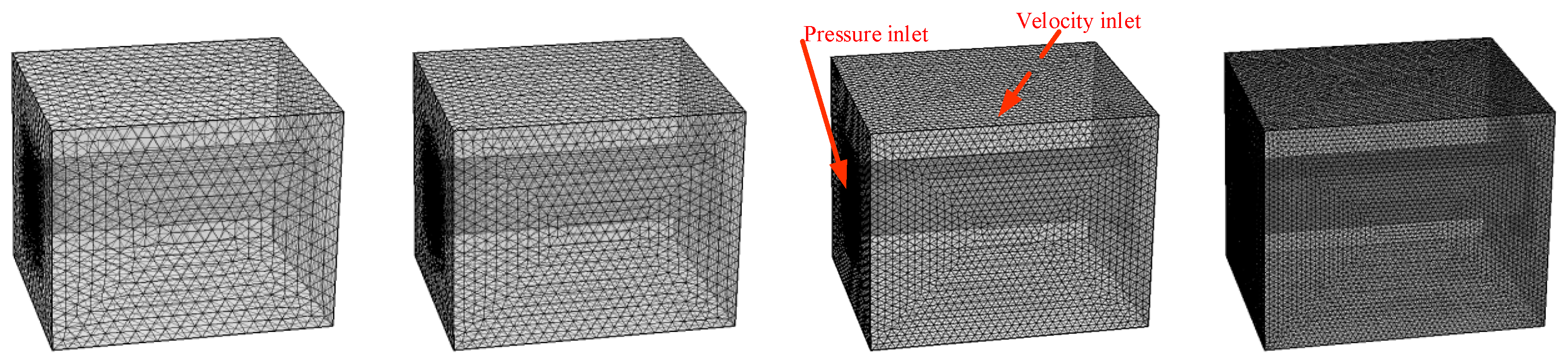
3.2. Geometric Model and Meshing of the Water Jet Flow Field

The size of the three-dimensional flow field was set to 5 m × 4 m × 4 m to investigate the effects of side wind on the properties of the jet flow field. When meshing, the mixed grid was applied in the computational domain (Figure 3), divided into two parts: the near-axis area through which the water jet flows, and the far-axis area away from the water jet. The scope of the paraxial area was 1 m. The above two areas had meshed independently. The near-axis area was meshed using a hexahedral grid with better calculation performance. The grid size increased gradually from the inside to the outside with a growth rate of 1.2, and the initial minimum edge length was 0.1 mm. The far-axis area was meshed using a tetrahedral–hexahedral mixed grid with a larger size, as shown in Figure 3.

At least four different grid calculations must be performed in order to analyze the grid convergence test, as show in Figure 3. As the mesh density increased, the velocity distribution on the axial section at the nozzle exit remained the same, and there was no significant difference. Furthermore, the change rate of the inlet and outlet pressure drop between adjacent grids was less than 0.9%. Therefore, the physical model and discrete format used in the calculation have spatial convergence and numerical stability, and the selection of a coarser grid number is sufficient to meet the accuracy requirements of the calculation.

3.3. Calculation Model and Governing Equation

After flowing through the contraction section of the nozzle, the high-speed water is turbulent, and turbulent diffusion and momentum exchange with the ambient air occurs violently [30]. Therefore, the nozzle jet belongs to the gas–liquid two-phase flow problem, and in the calculation of the jet flow field of the nozzle, the high-pressure water jet belongs to the state of high turbulence. Therefore, selecting a suitable turbulence model and multiphase flow model is necessary. The turbulence model selects standard k–ε governing equations.

The standard k–ε model is suitable for a flow field with low swirl intensity and regular wall shape, and it is a semi-empirical model based on model transport equations for the turbulent viscosity (μ_t), turbulent kinetic energy (κ), and its dissipation rate (ε), which are given by:

$${\mu }_t=\rho C_{\mu }\frac{k^2}{\epsilon }$$

(1)

$$\frac{\partial \left(\rho \kappa \right)}{\partial t}+\frac{\partial \left(\rho \kappa u_i\right)}{\partial x_i}=\frac{\partial }{\partial x_j}[\left(\mu +\frac{{\mu }_t}{{\sigma }_{\kappa }}\right)\frac{\partial \kappa }{\partial x_j}]+G_{\kappa }+G_b-\rho \epsilon -Y_M+S_{\kappa }$$

(2)

$$\frac{\partial \left(\rho \epsilon \right)}{\partial t}+\frac{\partial \left(\rho \kappa u_i\right)}{\partial x_i}=\frac{\partial }{\partial x_j}[\left(\mu +\frac{{\mu }_t}{{\sigma }_{\epsilon }}\right)\frac{\partial \epsilon }{\partial x_j}]+G_{1\epsilon }\frac{\epsilon }{\kappa }\left(G_{\kappa }+G_{3\epsilon }{G}_b\right)+G_{2\epsilon }\rho \frac{{\epsilon }^2}{\kappa }+S_{\epsilon }$$

(3)

where G_k represents the generation of turbulent kinetic energy due to the mean velocity gradients in these equations, G_b is the turbulent kinetic energy produced by buoyancy, and Y_M fluctuates due to excessive diffusion of incompressible turbulence. C_1ε, C_2ε, C_3ε, and C_μ are constants, σ_k and σ_ε are the turbulence Prandtl numbers for k and ε, respectively, and S_k and S_ε are user-defined. The model constants C_1ε, C_2ε, C_3ε, σ_k, and σ_ε were assumed to have the following values: C_1ε = 1.44, C_2ε = 1.92, C_μ = 0.09, σ_k = 1.0, and σ_ε = 1.3.

Since the VOF (volume of fluid) model is applicable to solve the spatiotemporal distribution of gas–liquid interface in stratified flow, sloshing, dam breaking, jet attenuation, etc. [31], the VOF model was selected for the multiphase flow model.

In the VOF model, the content of each phase fluid in each calculation unit is characterized by the volume fraction α. For example, in the case of q kinds of fluids, the volume fraction of each phase is α₁, α₂, …, α_q, and each volume fraction satisfies α₁ + α₂ + … + α_q = 1. The governing equations of the VOF model mainly include the volume fraction equation, momentum equation, and energy equation (Appendix A).

Assuming that the density changes of water and air can be ignored, the viscous flow in the computational domain is incompressible. The solver adopts the transient and pressure-based implicit solution, and the energy equation is opened to solve the jet temperature field simultaneously. The wall function in the standard k–ε turbulence model is set as the standard near-wall function. In the VOF two-phase model, the primary phase is air, and the secondary phase is water. The relationship between the physical parameters—such as thermal conductivity, viscosity, and specific heat capacity—and air and water temperatures is input into the material property column.

3.4. Boundary Conditions

The setting of boundary conditions of the computational domain is shown in Figure 3. The pressure reflects the nozzle outlet speed, and the relationship between them can be obtained from the literature [32]. Therefore, the nozzle inlet was set as the pressure inlet, and the pressure direction was perpendicular to the nozzle inlet surface. The turbulence intensity I and hydraulic diameter D_H of the inlet can be calculated by Equation (4):

$$\{\begin{array}{l}I=0.16\times {\left(R_{\mathrm{eD}}\right)}^{-1/8}\\ D_H=D\end{array}$$

(4)

where R_eD is the Reynolds number of the flow in the nozzle, and D_H is equal to the ratio of four times the flow area to the wetting circumference. D_H is the nozzle inlet diameter D for flows in a circular tube.

The volume fraction of water at the nozzle inlet was kept at 1, and the inlet temperature was set as the initial temperature of the hot water. The inner wall of the nozzle was set to have no sliding wall surface, and the wall material was set as steel. The nozzle outlet–air interface was set as the internal boundary. The front and back boundaries were selected as the velocity inlet in the external flow field area, used to simulate the transverse wind speed. The velocity direction was perpendicular to the jet axis. The upper and lower boundaries and the left and right boundaries were the pressure outlets. A pressure value was 0.1 MPa, one barometric pressure, and the temperature value was the ambient temperature. Before starting the calculation, the computational domain was initialized by filling the domain with air and setting the initial temperature as the ambient temperature.

For non-steady-state numerical simulation, it is necessary to determine the number of grids used, the time-step size, and the non-correlation with the calculation results—that is, the grids should be verified for non-correlation and time-independence. The four grid numbers were tested for independence according to the time step of 0.001 s.

After selecting the fixed number of grids, we set the Courant number to four levels from small, and chose the time step according to the convergence and error of the iterative residuals. In general, the Courant number is essential in explicit differential method schemes, and it should be small in order to ensure stability. The maximum control residual is 0.0001 in the iterative calculation. The numerical values used for the thermal parameters of water and air are shown in

Table 2. The numerical values used for the thermal parameters.

Properties	Density (kg/m3)	Cp (J/(kg K))	Thermal Conductivity (W/(m K))	Viscosity (kg/(m s))	Reference Temperature (°C)
Air	1.225	1006.43	0.0242	1.7894e-05	25
Water	998.2	4182	0.65	0.001003	24.85

.

4. Numerical Calculation Results and Validation of the Water Jet Flow Field

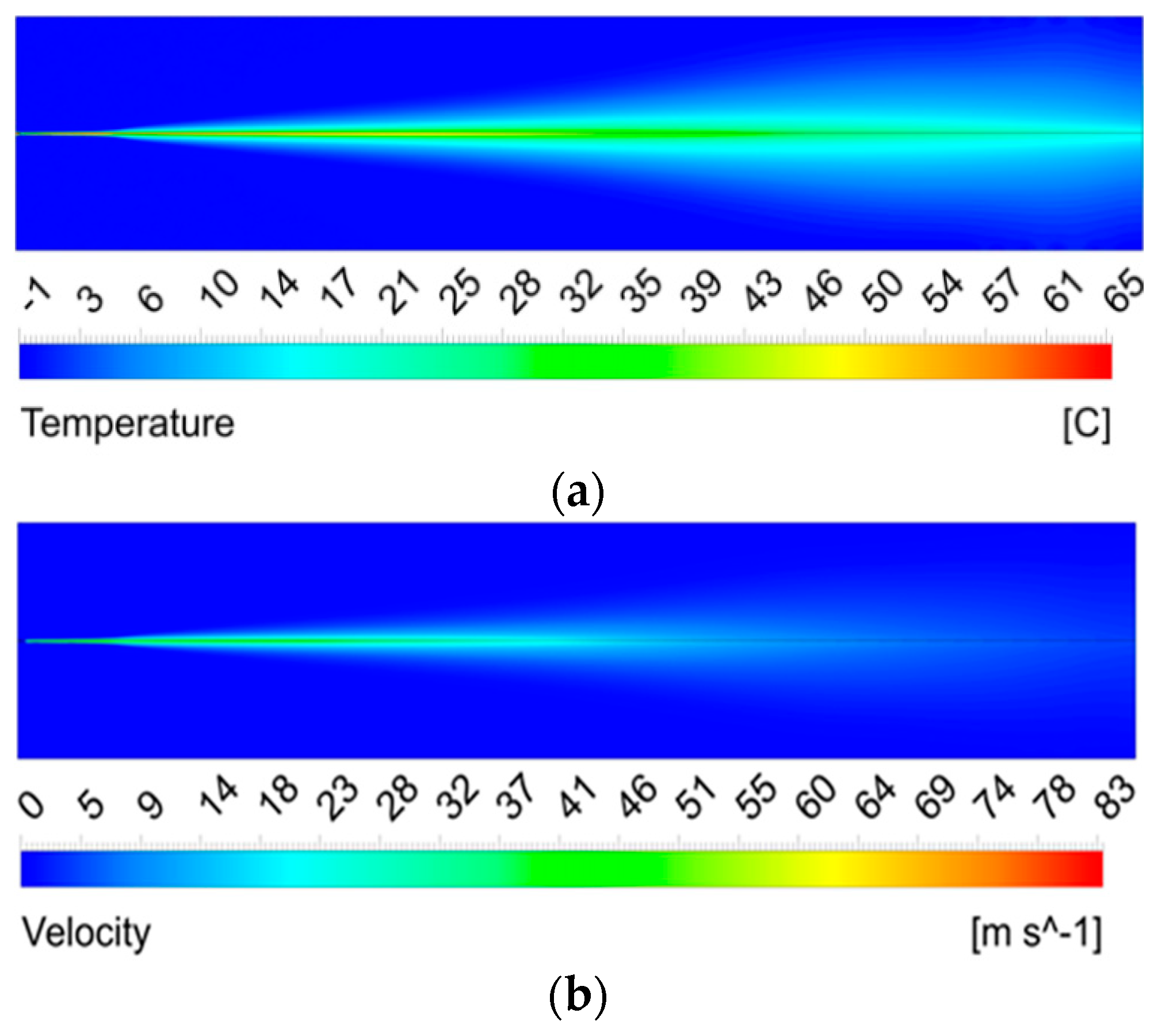
4.1. Numerical Calculation Results of Water Jet Flow Field

Taking the outlet pressure of 3 MPa as an example, when the wind speeds are 0 m/s and 3 m/s, the temperature and velocity contours of the water jet cross-section are shown in Figure 4 and Figure 5, respectively.

It can be seen from Figure 4 and Figure 5 that regardless of the presence of ambient wind, after the water jet sprays from the nozzle, the jet temperature and velocity gradually decrease along the axial direction, and the radial diffusion width gradually increases. Compared with 0 m/s, the core part of the temperature and velocity of the water jet is shifted along the direction of the wind speed due to the transverse wind blowing.

The temperature and velocity attenuation of the water jet are negatively correlated with the air entrainment along the way or the jet distance [33]. Figure 6 shows the velocity vector diagram at the nozzle outlet; the color difference represents the difference in speed. It can be seen from the figure that the high-speed water jet and the ambient air converge at the nozzle outlet, and the velocity value and direction of the two fluids are different. Under the entrainment of the longitudinal vortex [33], air approaches the main body of the water jet and turbulently moves forward with it, forming a gas–liquid two-phase mixed layer at the jet boundary. The violent momentum exchange and heat transfer occur between the entrained air and the water column, so the entrainment degree of the water jet is an essential factor affecting the jet’s temperature and velocity.

The velocity of the jet along the axis decays, and most of the energy is transferred to the surrounding fluid. The velocity of the jet body decreases, but more and more surrounding fluid moves forward together with the jet body under the entrainment of the longitudinal vortex, so that the flow rate of the jet fluid increases gradually along the path.

The mass entrainment rate J is defined to represent the entrainment degree of the jet to the air [34,35]; that is:

$$J=\frac{Q_x-Q_0}{Q_0}$$

(5)

where Q_x is the mass flow rate (kg/s) in the range where the minimal axial jet velocity is 0.5U_m on the radial cross-section at the distance of x away from the nozzle outlet, U_m is the maximum axial velocity on the radial cross-section (m/s), and Q₀ is the mass flow rate at the nozzle outlet (kg/s).

Figure 7 shows the mass entrainment rate and the axial distance when the outlet pressures are 4, 3, and 2 MPa. It can be seen from the figure that the mass entrainment rates under the three pressures increase with the increase in the axial distance and, especially when the distance x > 2.5 m, the mass entrainment rates increase rapidly. The above phenomenon indicates that, as the distance increases, more and more air is gradually entrained at the jet edge and approaches the center of the water jet. The edge of the water jet is “torn” by the air and gradually separates from the main body of the water column, forming a boundary layer with a lower velocity. Therefore, the jet’s temperature and velocity decrease progressively along the axis, and its diffusion width gradually increases.

4.2. Experimental Validation

The diffusion state of the water jet in the experiment is shown in Figure 8. The water column was photographed in sections with a high-speed camera to observe the internal flow of the water jet. The photographed results are shown in Figure 9 (test condition: the frame rate of the high-speed camera is 100 frames/second; in Figure 9a–c the nozzle diameter is 1.2 mm, and the outlet pressure is 1.5 MPa; Figure 9d shows the comparison of experimental results under different distance away from the nozzle, outlet pressures and nozzle diameters).

Time represents the acquisition time of a high-speed camera, which is in a steady state. Steady state refers to the obvious law of the water jet at this distance under the condition of a specific nozzle outlet, as can be obtained from the following results:

(1)

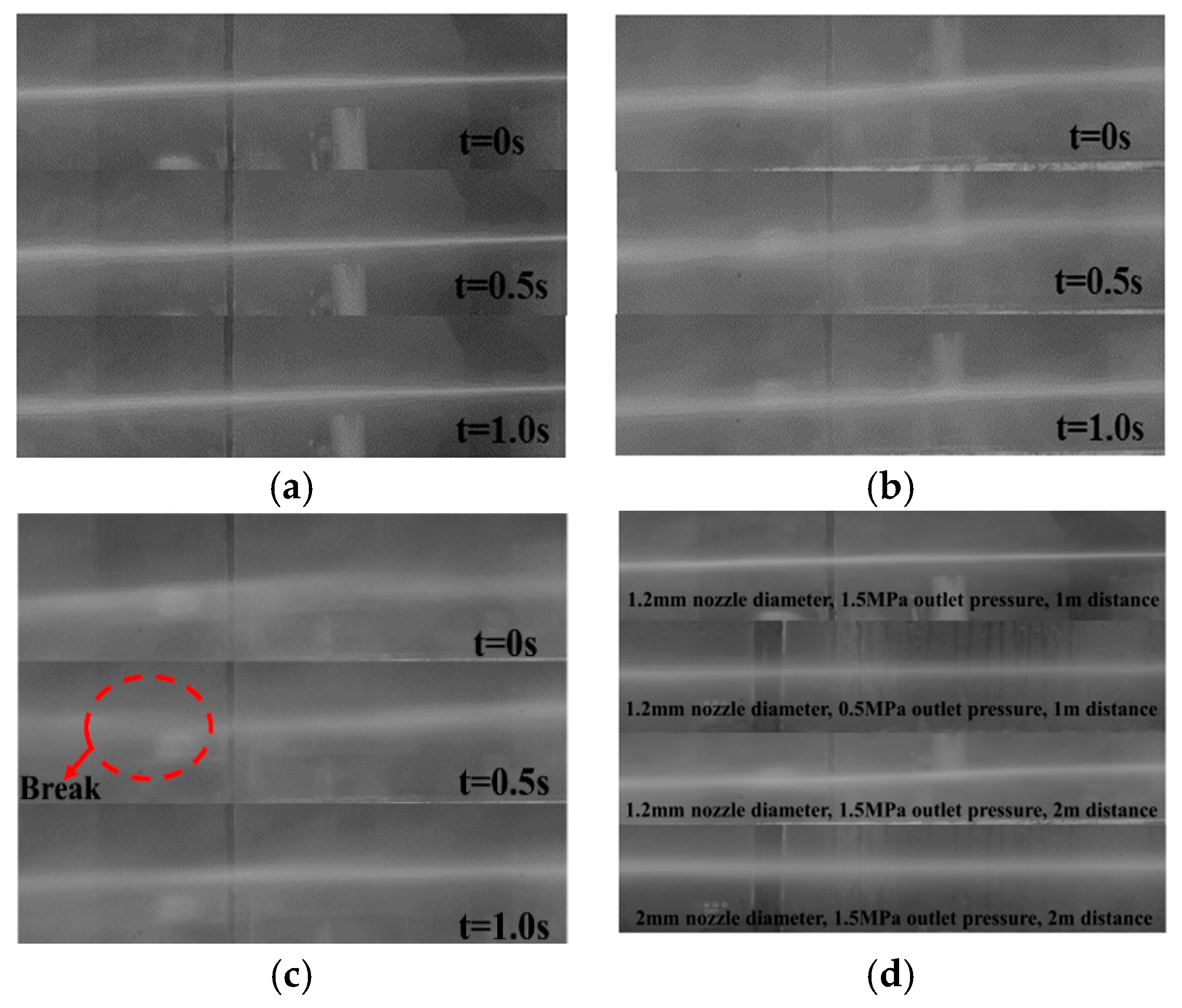
The distance affects the shape of the water jet. The water jet within 1 m is compact in Figure 9a, and the water column is straight, transparent, and dense. The cross-section width of the water column is clear, and the air is less mixed. According to the experiment results in Figure 9d, the compact segment’s length is related to the nozzle diameter and outlet pressure. To be specific, by comparing the water column states in the first two pictures, we can see that the compactness of the water column of 1.5 MPa is better, and the cross-section width of the water column is clearer than that at 0.5 MPa. Therefore, the length of the compact segment grows larger when the outlet pressure rises. Similarly, by comparing the water column states in the last two pictures, it can be seen that the water column of 2 mm nozzle diameter at 2 m is more compact than that of 1.2 mm nozzle diameter—that is, the compact segment extends as the nozzle diameter increases;

(2)

After the dense water column enters the air, it has strong friction with the air, the section widens, and the speed slows down. The water column is gradually doped with air, and the jet edge begins to diverge into water mist. The boundary layer of the water column gradually blurs, as shown in Figure 9b;

(3)

With the increase in distance, the jet entrains more air, causing the randomness of movement to become greater, and the water column diverges accordingly. For example, “break” occurs after the jet distance reaches 3 m in the condition of 1.2 mm nozzle diameter and 1.5 MPa outlet pressure, as shown in Figure 9c. With the increase in water jet injection distance, air entrainment intensifies, and the water column gradually absorbs air. Due to the doping of air, the motion of the water jet is slow and random, and the velocity is reduced to a slower speed. With the increase in jet length, the jet absorbs more and more air and is isolated into multiple water blocks by the air, resulting in a “break”;

(4)

Figure 9d shows that we have carried out experiments under different nozzle outlet conditions, and the test results show that the length of the water jet compact section is related to the nozzle diameter and the outlet pressure. Because the jet direction is from the right side to the left side of the picture, the water jet’s gravity effect is more obvious after the speed is reduced, resulting in the water jet state showing a low left and high right state.

The jet temperature was measured at different distances.

Table 3. The validation experiment parameters of water jet temperature.

Test Serial Number	Ambient Temperature (°C)	Average Wind Speed (m/s)	The Initial Temperature of Hot Water (°C)	Outlet Pressure (MPa)
1	2	3.4	80	2.2
2	0.2	3.9	65	3.0
3	1.5	4.7	55	4.0

shows the experimental conditions of each group. Each group was measured three times, and the average value was taken. The inlet and boundary conditions of the simulation model were set according to the experimental conditions, and the corresponding numerical calculation results were obtained. Since the temperature measured in the test was the average temperature of the water jet, it was necessary to integrate the radial temperature of the numerical results in order to obtain the average numerical calculation temperature T_ave.

$$T_{ave}=\frac{{\displaystyle \sum _1^n{T}_{\mathrm{i}}\cdot \Delta h}}{H}$$

(6)

where T_i is the temperature of the grid nodes, n is the number of grid nodes, Δh is the grid height, and H is the diffusion width of the water jet.

Figure 10 depicts a comparison between numerical results with experimental water jet temperature readings. It can be seen that the two are in excellent accordance, showing that the numerical water jet calculation model is reasonable and that the attenuation law of the water jet temperature may be derived from it. The difference is concentrated in 0–2 m and 4–5 m, because the entrainment rate of the jet increases with the increase in the axial distance—especially when the distance x > 2.5 m—and the mass entrainment rate increases rapidly.

At the same time, in order to verify the rationality of the numerical calculation of water jet velocity, the simulation calculation of the axial velocity of a 1.5 mm nozzle at outlet pressures of 4, 3, and 2 MPa was carried out. The comparison between the calculated value of the normalized axial velocity U_m/U₀ at different distances and the experimental value is shown in Figure 11, where U_m is the maximum axial velocity on the radial cross-section (m/s), and U₀ is the velocity at the nozzle outlet (m/s).

The following can be seen from Figure 11:

(1)

Under the three outlet pressures, although the velocity at the nozzle outlet is different, the attenuation law of the normalized axial velocity along the axial direction is virtually the same;

(2)

The fluid velocity at the nozzle inlet is low. The velocity increases sharply after the conical contraction section, and reaches its maximum at the nozzle outlet. The jet velocity gradually decreases after leaving the nozzle, and the velocity decays rapidly within a short distance from the nozzle outlet, and then approximately declines linearly;

(3)

Taking the numerical result of 4 MPa as an example, when x = 1000d—that is, 1.5 m away from the nozzle outlet—the axial velocity U_m = 57.11 m/s, which decreases to 64.73% of the outlet velocity (U₀ = 88.23 m/s). When x = 2500d—that is, 3.75 m away from the nozzle outlet—the axial velocity U_m = 22.25 m/s, which decreases to 25.22% of the outlet velocity U₀. The numerical simulation results agree well with the experimental results in the literature [36,37]; that is, the axial velocity of the water jet shows linear attenuation, and the axial velocity is ~0.7U₀ at 1000d and ~0.25U₀ at 2500d.

In summary, the relative error between the numerically calculated results of water jet temperature and axial velocity and the experimental result is small. Therefore, the simulation calculation of the water jet in this paper can reflect the characteristics of the water jet flow field well, and the reliability of the numerical calculation model is validated.

According to the optimization method given in the literature [27], the optimal deicing effect parameters in a specific environment can be obtained. For the 1.2 mm diameter nozzle, the ambient temperature is −3 °C, the wind speed is 3 m/s, the icing weight is 2 kg/piece, and the distance is 2 m. The optimal initial hot water temperature and jet outlet pressure values are 86.07 °C (35–100 °C) and 3.49 MPa (1–7 MPa), respectively. The total deicing efficiency is optimal when the hot water outlet temperature is around 86 °C and the jet pressure is around 3.5 MPa.

5. Analysis of Factors Affecting the Spatial Distribution of Water Jet Temperature

5.1. The Effect of the Initial Temperature of the Hot Water

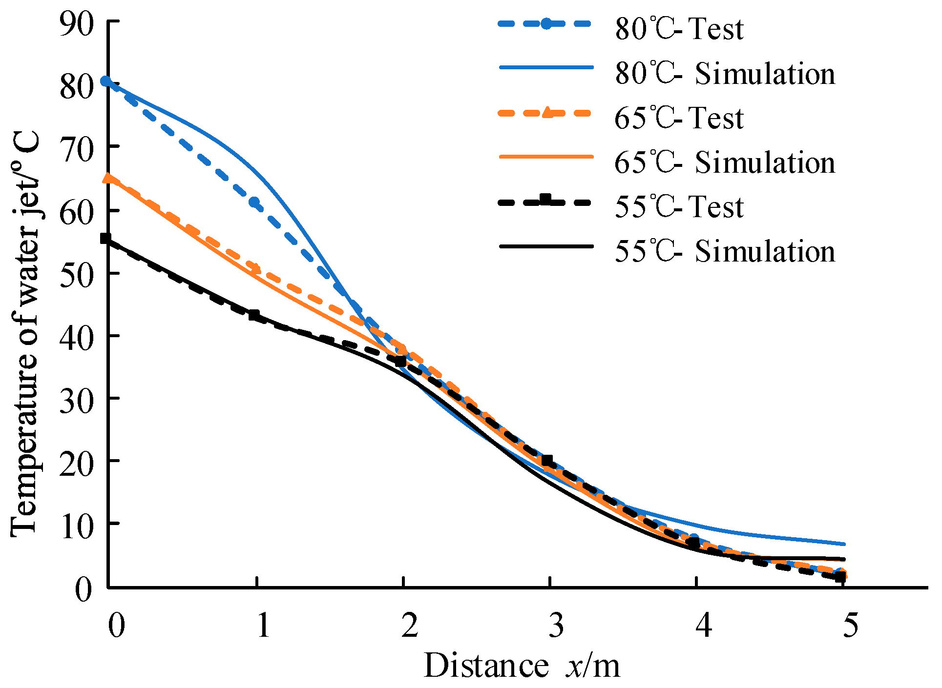
In order to ascertain the relationship between the water jet temperature at different distances and the initial temperature, the test conditions were set as 1.2 mm, −1 °C, 3 m/s, and 3 MPa (from left to right are the nozzle diameter, ambient temperature, wind speed, outlet pressure, and the same below), and the results are shown in Figure 12.

The following can be concluded from the above Figure:

(1)

The temperature of the water jet is positively correlated with the hot water’s initial temperature. Compared with 35 °C, the water temperatures of 50–95 °C increased the jet temperature by 33.67%, 86.73%, 119.48%, and 172.82%, showing an approximately linear increase;

(2)

The rate of water jet temperature increase with the initial temperature of the hot water is negatively correlated with distance—that is, the longer the distance, the lower the growth rate. As shown in Figure 12, when the distance increases from 1 m to 5 m, the increase rate of the jet temperature decreases from 0.72 to 0.06. With the increase in the jet distance, the difference between the initial temperature of the hot water and the temperature when it reaches the ice layer becomes larger—that is, the effect of the former weakens.

5.2. The Effect of Jet Distance

In order to study the change rule of water jet temperature in the axial direction, the test conditions were set as 1.2 mm, −1 °C, 3 m/s, and 4 MPa in order to ascertain the temperature of the water jet at different distances.

As shown in Figure 13, the temperature of the water jet is negatively correlated with the distance when the environmental parameters remain constant.

5.3. The Effect of Outlet Pressure

The outlet pressure was set as 2 MPa, 3 MPa, and 4 MPa, the ambient temperature was –1 °C, and the wind speed was 3 m/s. The relationship between the temperature at 2 m and the outlet pressure at different initial temperatures of hot water was determined, as shown in Figure 14.

As can be seen from Figure 14, the water jet temperature decreases slightly with outlet pressure. Compared with 2 MPa, the temperatures at 3 MPa and 4 MPa were reduced by 3.66% and 7.49%, respectively.

The temperature change of the water jet in the air is a convective heat transfer problem. According to the literature [21,38], this kind of problem can be qualitatively analyzed based on the following equations:

$$q^{″}=h\left(T_{\mathrm{s}}-T_{\infty }\right)\hspace{0.17em}\hspace{0.17em}\hspace{0.17em}h=k{N}_u/L\hspace{0.17em}\hspace{0.17em}\hspace{0.17em}\mathrm{Re}=\frac{L{u}_{\infty }}{\nu }$$

(7)

where q″ is the convective heat flux, representing the convective heat transfer in units of time; h is the convective heat transfer coefficient; T_s is the water jet temperature; T_∞ is the air temperature; k is the thermal conductivity of air; L is the heat transfer characteristic length, here referring to jet distance; the Nusselt number Nu is positively correlated with the Reynolds number Re; u_∞ is the relative velocity between the water jet and the air, which is mainly determined by outlet pressure and wind speed; and v is the kinematic viscosity of air.

When other factors such as ambient temperature and wind speed remain constant, u_∞ increases as the outlet pressure increases. This causes the Reynolds number Re, the convective heat transfer coefficient h, and convective heat flux q″ to increase accordingly at the same distance from the nozzle outlet. The increase in q″ means more heat is transferred from the water jet to the ambient air within the same time. Therefore, the water jet temperature decreases with the rise in the outlet pressure.

5.4. The Effect of Ambient Temperature

Taking the conditions of −1 °C, 0 m/s, and 3 MPa as the control group, the simulation conditions of the other four groups were −7, −6, −4, and −2 °C, respectively. The water jet temperature at different ambient temperatures is shown in Figure 15.

When the initial temperature of hot water and the ambient wind speed are constant, the temperature of the water jet decreases with the decrease in the ambient temperature, which is generally linear. Each time the ambient temperature decreases by 1 °C under this condition, the water temperature decreases by approximately 0.375 °C.

It can be speculated from Equation (4) that as the ambient temperature T_∞ drops, the temperature difference T_s–T_∞ between the water jet and the air increases. At the same time, the effect of the ambient temperature change (from −7 °C to −1 °C) on the convective heat transfer coefficient h can be ignored. Therefore, the convective heat flux q″ increases and, thus, the water jet temperature decreases with the decrease in the ambient temperature.

At the same time, by comparing the slopes of the curves at different distances, it can be seen that the further the distance, the faster the water temperature will rise with the increase in ambient temperature. The ambient temperature change at close range has almost no effect on the water jet temperature. The air content in water jets may cause this variation trend to rise with the increasing distance.

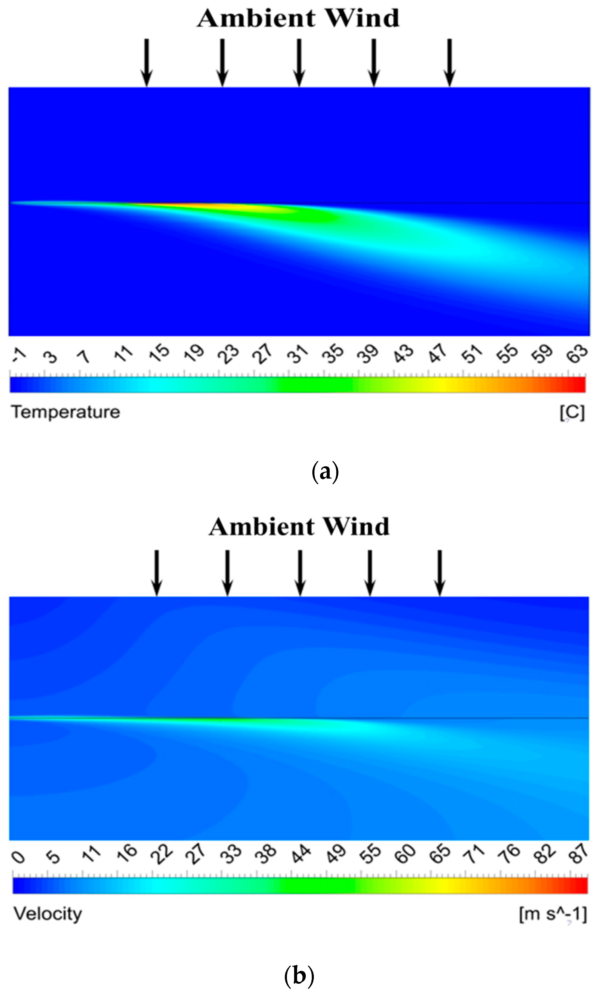
5.5. The Effect of Environmental Wind Speed

To study the degree of influence of wind speed on the attenuation of the water jet temperature, the conditions of −1 °C, 0 m/s, and 3 MPa were taken as the control group, and the other two groups were −1 °C, 1.5 m/s, 3 MPa and −1 °C, 3 m/s, 3 MPa. The relationship between water jet temperature and wind speed was calculated, as shown in Figure 16.

As shown in Figure 16, when the initial temperature of the hot water and the ambient temperature are constant, the temperature of the water jet decreases as the wind speed increases. Compared with the windless condition, the water jet temperatures of 1.5 m/s and 3 m/s reduced by 7.59% and 13.46%, respectively.

The effect of wind speed on the water jet temperature is greater than that of the ambient temperature. For example, when the initial temperature of the hot water is 95 °C, compared with the calculated result of the control group (−1 °C, 0 m/s), as the ambient temperature decreases by 3 °C, the temperature of water jet at 3 m drops from 49.15 °C to 47.9 °C, which is a decrease of 1.25 °C. However, when the ambient wind speed increases by 3 m/s, the temperature of the water jet at 3 m decreases by 16.23 °C.

When the wind speed increases, the relative velocity u_∞ between the water jet and the air increases, which eventually causes the heat loss of the water jet to increase within the same time. Moreover, according to our field tests on water jets in windy conditions, it appears that the compactness of the water column becomes worse with increasing wind speed. The mixing of air into a water jet would enhance the convective heat transfer and, thus, accelerate the attenuation of the water jet temperature. Therefore, the temperature of the water jet decreases as the wind speed increases, and the increase in wind speed has a more significant impact on the water jet temperature than the decrease in ambient temperature.

5.6. The Effect of Nozzle Diameter

Taking three nozzle diameters of 1.2 mm, 1.5 mm, and 2 mm as examples, the relationship between water jet temperature and nozzle diameter at 2 m was calculated under the boundary conditions of 1.5 MPa outlet pressure, with environmental parameters of −1 °C and 0 m/s, as shown in Figure 17.

Increasing nozzle diameter can improve water jet temperature when the other parameters are the same. Since air damages the water column structure from the outer layer to the inner core, the thicker water column has a greater ability to withstand damage to its core, and a better ability to retain heat. Therefore, when the initial temperature of the hot water is constant, the larger the nozzle diameter, the smaller the temperature drop would be at the same distance.

For example, when the nozzle diameter increases from 1.2 mm to 2 mm, the water jet temperatures at 2 m distance of 80 °C, 65 °C, and 45 °C initial temperature increase from 54.32 °C, 46.41 °C, and 30.87 °C to 63.15 °C, 54.02 °C, and 40.58 °C respectively, with increases of 16.27%, 16.40%, and 31.45%. The lower the initial temperature of the hot water, the more the nozzle diameter will increase the temperature of the water jet.

6. Conclusions

This paper studied the characteristics of a hot water jet in the air. The numerical calculation model of the water jet flow field was established and verified. The effects of the initial temperature of the hot water, jet distance, outlet pressure, nozzle diameter, ambient temperature, and wind speed on water jet temperature were studied. The main conclusions are as follows:

(1)

The water column in the initial segment of the water jet is compact. The increase in distance will cause the water jet to diverge gradually, and the boundary layer will become blurred. After reaching a certain distance, the water jet “breaks”;

(2)

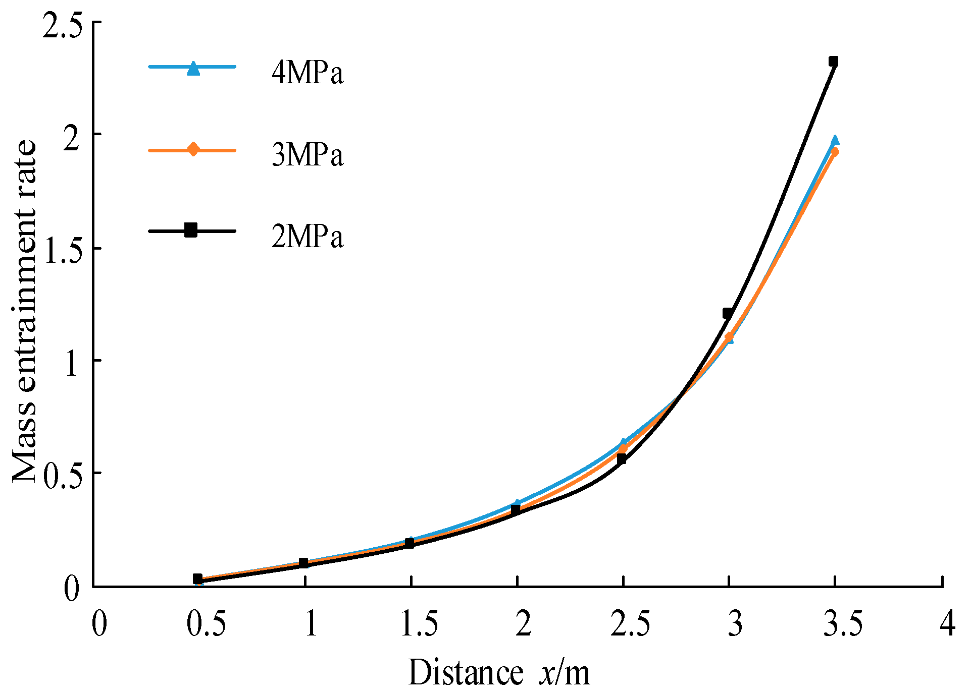
The numerical results of the hot water jet calculations are consistent with the results of the field studies. The mass entrainment of the water jet increases with the increasing distance. Under the three outlet pressures, the attenuation law of normalized axial velocity of the water jet along the axial direction is the same, and decreases approximately linearly. When the distance x = 1000d, U_m = 0.63U₀, and when the distance x = 2500d, U_m = 0.25U₀;

(3)

The water jet temperature is negatively correlated with distance and outlet pressure, and the distance has a greater impact. The water jet temperature is positively correlated with the initial temperature of the hot water, and the increase in distance will weaken the influence of the initial temperature of the hot water. When the ambient temperature and wind speed change the same value, the wind speed is greater than the ambient temperature. Increasing the nozzle diameter can increase the flow rate, effectively increasing the water jet temperature. According to the effective laws of the above factors on the spatial distribution of water jet temperature, the optimal parameter for ice melting can be obtained theoretically, which will be discussed in future work.

The convective heat transfer coefficient between the water jet and ice is more significant than that between hot air and ice at the same flow velocity; therefore, hot water deicing has great advantages over laser deicing. In addition, based on the results of the water jet research in this paper, the efficiency of hot water deicing can be further optimized. Furthermore, the water jet properties may also have other applications, such as the generation of a photoacoustic effect [39,40,41], water jet cutting [42], trenching the seafloor using specifically designed water jetting tools [43], deburring technology, or cavitation [44,45].

References

1. Yin, F.; Farzaneh, M.; Jiang, X. Electrical characteristics of an energized conductor under various weather conditions. High Volt. 2017, 2, 102–109. [Google Scholar] [CrossRef]
2. Ale-Emran, S.M.; Farzaneh, M. Flashover performance of ice-covered post insulators with booster sheds using experiments and partial arc modeling. IEEE Trans. Dielectr. Electr. Insul. 2016, 23, 979–986. [Google Scholar] [CrossRef]
3. Hu, Q.; Wang, S.; Shu, L.; Jiang, X.; Liang, J.; Qiu, G. Comparison of AC icing flashover performances of 220 kV composite insulators with different shed configurations. IEEE Trans. Dielectr. Electr. Insul. 2016, 23, 995–1004. [Google Scholar] [CrossRef]
4. Farzaneh, M.; Chisholm, W.A. 50 years in icing performance of outdoor insulators. IEEE Electr. Insul. Mag. 2014, 30, 14–24. [Google Scholar] [CrossRef]
5. Jiang, X.; Fan, C.; Xie, Y. New method of preventing ice disaster in power grid using expanded conductors in heavy icing area. IET Gener. Transm. Distrib. 2019, 13, 536–542. [Google Scholar] [CrossRef]
6. Jiang, X.; Xiang, Z.; Zhang, Z.; Hu, J.; Hu, Q.; Shu, L. Predictive Model for Equivalent Ice Thickness Load on Overhead Transmission Lines Based on Measured Insulator String Deviations. IEEE Trans. Power Deliv. 2014, 29, 1659–1665. [Google Scholar] [CrossRef]
7. Hu, Q.; Yuan, W.; Shu, L.; Jiang, X.; Wang, S. Effects of electric field distribution on icing and flashover performance of 220 kV composite insulators. IEEE Trans. Dielectr. Electr. Insul. 2014, 21, 2181–2189. [Google Scholar] [CrossRef]
8. Polhman, J.C.; Landers, P. Present state-of-the-art of transmission line icing. IEEE Trans. Power Appar. Syst. 1982, 101, 2443–2450. [Google Scholar] [CrossRef]
9. Losowski, E.P.; Gayet, J.F. Atmospheric icing: A review. Process. IWAIS 1988, 3, 1–6. [Google Scholar]
10. Laforte, J.; Allaire, M.; Laflamme, J. State-of-the-art on power line de-icing. Atmos. Res. 1998, 46, 143–158. [Google Scholar] [CrossRef]
11. Chang, G.; Su, S.; Li, M.; Chao, D. Novel Deicing Approach of Overhead Bundled Conductors of EHV Transmission Systems. IEEE Trans. Power Deliv. 2009, 24, 1745–1747. [Google Scholar] [CrossRef]
12. Farzaneh, M.; Jakl, F.; Arabani, M.P.; Eliasson, A.J.; Fikke, S.M.; Gallego, A.; Haldar, A.; Isozaki, M.; Lake, R.; Leblond, L. Systems for Prediction and Monitoring of Ice Shedding, Anti-Icing and De-Icing for Power Line Conductors and Ground Wires; CIGRE: Paris, France, 2010; p. 438. [Google Scholar]
13. Yan, B.; Chen, K.; Guo, Y.; Liang, M.; Yuan, Q. Numerical Simulation Study on Jump Height of Iced Transmission Lines After Ice Shedding. IEEE Trans. Power Deliv. 2012, 28, 216–225. [Google Scholar] [CrossRef]
14. Chen, Y.; Wang, Q.; Gu, B.; Cai, Y.; Wen, F. Research on the operating process of DC De-icer and its De-icing efficiency in China Southern Power Grid. In Proceedings of the 2012 10th International Power & Energy Conference (IPEC), Ho Chi Minh City, Vietnam, 12–14 December 2012; pp. 583–588. [Google Scholar]
15. Wei, S.; Wang, Y.; Yang, Y.; Yin, F.; Cao, W.; Tang, Y. Applying Q-learning Algorithm to Study Line-Grasping Control Policy for Transmission Line Deicing Robot. In Proceedings of the 2010 International Conference on Intelligent System Design and Engineering Application, Changsha, China, 13–14 October 2010; pp. 382–387. [Google Scholar]
16. Zhu, W. Research on De-Icing of Power Line Using CO2 Laser. Master’s Thesis, School of Optoelectronic Science and Engineering, Huazhong University of Science and Technology, Wuhan, China, 2007. [Google Scholar]
17. Qi, L.; Zhu, X.; Guo, F.; Gu, S. Deicing with Nd:YAG and CO2 lasers. Opt. Eng. 2010, 49, 114301. [Google Scholar] [CrossRef]
18. Xie, T.; Dong, J.; Chen, H.; Jiang, Y.; Yao, Y. Experiment investigation on de-icing characteristics and energy efficiency using infrared ray as heat source. Energy 2016, 116, 998–1005. [Google Scholar] [CrossRef]
19. Li, B.; He, L.; Liu, Y.; Zhang, G. Influences of key factors in hot-air de-icing for live substation equipment. Cold Reg. Sci. Tech. 2019, 160, 89–96. [Google Scholar] [CrossRef]
20. Xie, T.; Dong, J.; Chen, H.; Jiang, Y.; Yao, Y. Experimental investigation of de-icing characteristics using hot air as heat source. Appl. Therm. Eng. 2016, 107, 681–688. [Google Scholar] [CrossRef]
21. Incropera, F.P.; Dewitt, D.P. Fundamentals of Heat and Mass Transfer; John Wiley & Sons Press: New York, NY, USA, 2007. [Google Scholar]
22. Takahashi, K.; Usami, N.; Shibata, T.; Goto, K.; Uehara, T.; Kondo, H.; Ishikawa, R.; Saeki, H. Experimental study on a deicing method using a water jet. In Proceedings of the Oceans ′04 MTS/IEEE Techno-Ocean ′04 (IEEE Cat. No.04CH37600), Kobe, Japan, 9–12 November 2004; pp. 1668–1673. [Google Scholar]
23. Guo, Z.; Long, X.; Liu, Q.; Zhang, M. Experimental study on water-jet de-icing. In Proceedings of the 2014 ISFMFE—6th International Symposium on Fluid Machinery and Fluid Engineering, Wuhan, China, 22–22 October 2014; pp. 1–4. [Google Scholar]
24. Zhu, Z.; Zhang, X.; Wang, Q.; Chu, W. Research and experiment of thermal water de-icing device. Trans. Can. Soc. Mech. Eng. 2015, 39, 783–788. [Google Scholar] [CrossRef]
25. Zhou, J.Z.; Xu, X.P.; Chu, W.J.; Dai, J.Y.; Chen, Y.H.; Zhu, Z.C.; Lai, S.W. R&D of a New De-Icing Device Based on Synthetically De-Icing Techniques. Appl. Mech. Mater. 2013, 372, 381–386. [Google Scholar] [CrossRef]
26. Ji, C. Experimental Research and Simulation Analysis for EMU de-icing method. Master’s Thesis, Mechanical Engineering Tianjin University, Tianjin, China, 2012. [Google Scholar]
27. Zhang, Z.; Yang, S.; Jiang, X.; Ma, X.; Huang, H.; Pang, G.; Ji, Y.; Dong, K. Hot Water Deicing Method for Insulators Part 2: Analysis of Ice Melting Process, Deicing Efficiency and Safety Distance. IEEE Access 2020, 8, 130729–130739. [Google Scholar]
28. Wen, J.; Qi, Z.; Behbahani, S.S.; Pei, X.; Iseley, T. Research on the structures and hydraulic performances of the typical direct jet nozzles for water jet technology. J. Braz. Soc. Mech. Sci. Eng. 2019, 41, 570. [Google Scholar] [CrossRef]
29. Zhou, J.Z.; Xu, X.P.; Chu, W.J.; Zhu, Z.C.; Chen, Y.H.; Lai, S.W. Analysis and Simulation of the Fluid Field in Thermal Water-Jet Nozzle Based on ANSYS FLUENT & ICEM CFD. Appl. Mech. Mater. 2013, 423–426, 1677–1684. [Google Scholar] [CrossRef]
30. Guha, A.; Barron, R.M.; Balachandar, R. Numerical simulation of high-speed turbulent water jets in air. J. Hydraul. Res. 2010, 48, 119–124. [Google Scholar] [CrossRef]
31. Srinivasan, V.; Salazar, A.J.; Saito, K. Modeling the disintegration of modulated liquid jets using volume-of-fluid (VOF) methodology. Appl. Math. Model. 2011, 35, 3710–3730. [Google Scholar] [CrossRef]
32. Tikhomirov, R.A.; Petukhov, E.N.; Babanin, V.F. High-Pressure Jet Cutting; ASME Press: New York, NY, USA, 1992. [Google Scholar]
33. Turner, J.S. Turbulent entrainment: The development of the entrainment assumption, and its application to geophysical flows. J. Fluid Mech. 1986, 173, 431–471. [Google Scholar] [CrossRef]
34. Yu, Y.; Li, X.; Meng, H.; Wang, Y.; Song, M.; Wu, J. Jet flow and entrainment characteristics of nozzles with different shapes. Chin. J. Process Eng. 2014, 14, 549–555. [Google Scholar]
35. Li, D.; Fan, J.; Cen, K. Direct numerical simulation of the entrainment coefficient and turbulence properties for compressible spatially evolving axisymmetric jets. Fuel 2012, 102, 470–477. [Google Scholar] [CrossRef]
36. Rajaratnam, N.; Rizvi, S.A.H.; Steffler, P.M.; Smy, P.R. An experimental study of very high velocity circular water jets in air. J. Hydraul. Res. 1994, 32, 461–470. [Google Scholar] [CrossRef]
37. Guha, A.; Barron, R.M.; Balachandar, R. An experimental and numerical study of water jet cleaning process. J. Mater. Process. Technol. 2011, 211, 610–618. [Google Scholar] [CrossRef] [Green Version]
38. Holman, J.P. Heat Transfer; China Machine Press: Beijing, China, 2011. [Google Scholar]
39. Pang, G.A.; Laufer, J.; Niessner, R. Photoacoustic Signal Generation in Gold Nanospheres in Aqueous Solution: Signal Generation Enhancement and Particle Diameter Effects. J. Phys. Chem. C 2016, 6, 09374. [Google Scholar] [CrossRef]
40. Gandolfi, M.; Banfi, F.; Glorieux, C. Optical wavelength dependence of photoacoustic signal of gold nanofluid. Photoacoustics 2020, 20, 100199. [Google Scholar] [CrossRef]
41. Chen, Y.S.; Frey, W.; Kim, S. Silica-Coated Gold Nanorods as Photoacoustic Signal Nanoamplifiers. Nano Lett. 2011, 11, 348–354. [Google Scholar] [CrossRef] [PubMed]
42. Yuyong, L.; Puhua, T.; Daijun, J.; Kefu, L. Artificial neural network model of abrasive water jet cutting stainless steel process. In Proceedings of the 2010 International Conference on Mechanic Automation and Control Engineering, Wuhan, China, 26–28 June 2010; pp. 3507–3511. [Google Scholar] [CrossRef]
43. Li, J.H.; Kim, J.T.; Lee, M.J.; Jee, S.C.; Kang, H.J.; Kim, M.K.; Kwak, H.W.; Kim, S.B.; Oh, T.W. Water jetting arm optimal design consideration for a ROV trencher. In Proceedings of the OCEANS 2015—Genova, Genova, Italy, 18–21 May 2015; pp. 1–5. [Google Scholar] [CrossRef]
44. Wang, G.; Senocak, I.; Shyy, W.; Ikohagi, T.; Cao, S. Dynamics of attached turbulent cavitating flows. Prog. Aerosp. Sci. 2001, 37, 551–581. [Google Scholar] [CrossRef]
45. Sun, Z.; Kang, X.; Wang, X. Experimental system of cavitation erosion with water-jet. Mater. Des. 2004, 26, 59–63. [Google Scholar] [CrossRef]
Figure 1. Hot water deicing process of an LXY-120 glass insulator. (a) Process from 0 s to 120 s at 30 s intervals; (b) Ice falling off.
Energies 15 02298 g001
Figure 2. Schematic diagram of the nozzle structure.
Energies 15 02298 g002
Figure 3. Different meshing and boundary condition settings of the water jet flow field.
Energies 15 02298 g003
Figure 4. The numerical calculation results of the water jet when the ambient wind speed is 0 m/s: (a) The temperature contour of the water jet. (b) The velocity contour of the water jet.
Energies 15 02298 g004
Figure 5. The numerical calculation results of the water jet when the ambient wind speed is 3 m/s: (a) The temperature contour of the water jet. (b) The velocity contour of the water jet.
Energies 15 02298 g005
Figure 6. Enlarged view of the velocity vector at the nozzle outlet.
Energies 15 02298 g006
Figure 7. Mass entrainment rates under different outlet pressures.
Energies 15 02298 g007
Figure 8. The diffusion state of the water jet.
Energies 15 02298 g008
Figure 9. The state of the water jet (high-speed photography): (a) 1 m; (b) 2 m; (c) 3 m; (d) Comparison of experimental results under different distance away from the nozzle, outlet pressures and nozzle diameters.
Energies 15 02298 g009
Figure 10. Comparison between experimental and simulation values of water jet temperature.
Energies 15 02298 g010
Figure 11. Comparison between numerical calculation results and experimental value (References [36,37]) of axis velocity.
Energies 15 02298 g011
Figure 12. Relationship between water jet temperature and the initial temperature of the hot water.
Energies 15 02298 g012
Figure 13. Relationship between water jet temperature and distance.
Energies 15 02298 g013
Figure 14. Relationship between the temperature of the water jet and the pressure at the outlet.
Energies 15 02298 g014
Figure 15. Relationship between water jet temperature and ambient temperature.
Energies 15 02298 g015
Figure 16. Relationship between water jet temperature and wind speed.
Energies 15 02298 g016
Figure 17. Relationship between water jet temperature and nozzle diameter.
Energies 15 02298 g017