Article

Multi-Objective Optimisation for Large-Scale Offshore Wind Farm Based on Decoupled Groups Operation

1
School of Electronic and Information Engineering, Jiujiang University, Jiujiang 332005, China
2
School of IT Information and Control Engineering, Kunsan National University, Kunsan 54150, Korea
3
School of Automation, Central South University, Changsha 410083, China
*
Author to whom correspondence should be addressed.
Energies 2022, 15(7), 2336; https://doi.org/10.3390/en15072336
Submission received: 18 February 2022 / Revised: 17 March 2022 / Accepted: 18 March 2022 / Published: 23 March 2022
(This article belongs to the Special Issue Modern Technologies for Renewable Energy Development and Utilization)

Abstract

:
Operation optimization for large-scale offshore wind farms can cause the fatigue loads of single wind turbines to exceed their limits. This study aims to improve the economic profit of offshore wind farms by conducting multi-objective optimization via decoupled group operations of turbines. To do this, a large-scale wind farm is firstly divided into several decoupled subsets through the parallel depth-first search (PDFS) and hyperlink-induced topic search (HITS) algorithms based on the wake-based direction graph. Next, three optimization objectives are considered, including total output power, total fatigue load, and fatigue load dispatch on a single wind turbine (WT) in a wind farm. And then, the combined Monte Carlo and beetle swarm optimization (CMC-BSO) algorithms are applied to solve the multi-objective non-convex optimization problem based on the decentralized communication network topology. Finally, the simulation results demonstrate that the proposed method balances the total power output, fatigue load, and single fatigue loads with fast convergence.

1. Introduction

There are many studies on wind turbines of on-shore and offshore turbines [1,2,3,4,5]. However, in order to capture more power, various researchers have proposed a method to construct wind farms by placing many turbines together, either onshore or offshore [6,7]. In recent years, offshore wind farms (OWFs) have been increased in popularity due to the steadier and higher wind speeds, fewer land space limitations, and lower amounts of noise pollution as compared with onshore wind farms [8]. However, the major challenge in OWFs is their noticeably higher cost than their onshore counterparts, to which operation and maintenance costs (O&M) contribute a considerable amount [9]. OWF owners take advantage of large-scale economies by erecting many turbines together to save investment costs. A large-scale OWF often consists of dozens or even hundreds of wind turbines (WTs). In these cases, the wake effect cannot be ignored, as it significantly impacts the economic performance of OWF in terms of decreasing the power output and increasing fatigue loads [10]. To increase the economic profits, operating OWFs can be improved by focusing on the following three aspects: (1) communication topology; (2) optimization objective; (3) optimization solver.
It is particularly important to design the communication topology for a large-scale OWF. There are various communication topologies, such as centralized, distributed, decentralized, or a combination. For a centralized topology, the central controller deals with all the information from the wind turbines and makes decisions for each wind turbine. The traditional centralized controller has gradually encountered a heavy computational burden due to the larger dimensions and higher complexity of the calculation [11]. For this reason, a centralized framework may not be practical because of its high construction cost and communication costs [11]. Conversely, the non-centralized topology can relieve the communication burden as wind turbines are equipped with a controller that communicates solely with the turbines in each subset and the supervisor. Various turbines are shared between the subsets in the distributed topology, which creates a challenge for the optimization solver in terms of dealing with information sharing related to the wake propagations [12,13]. On this basis, the decentralized topology was proposed to divide a large-scale wind farm into various decoupled subsets, making it easy to reach the global optimization value for each controller. However, it is necessary to find a suitable method to design a decentralized communication topology by dividing wind turbines into several decoupled subsets [14,15]. For example, Hankel singular values and selective modal analysis were studied in [16,17]. However, they did not consider the wake effect. Various researchers presented clustering the WTs into several groups according to their wind profiles; thus, all turbines in the same group can be treated as one single turbine. However, it is difficult to implement during the actual operation because the wind profiles are time-varying [14]. Another nearest-neighbor method was proposed to group the OWF into several clusters, in which a wind turbine is only communicated with neighbor turbines [11,18]. However, the wind direction was assumed to be constant, thus it is hard to utilize with varying wind directions. Motivated by this, various researchers have proposed the concept of a wake effect digraph to characterize the wake, and decoupling techniques were designed to decouple the wake digraph [15,19]. Although these algorithms can ease the computational workload to a certain extent, efficient decentralized methods need to be explored based on the wake effect.
Increasing the performance of OWF by decreasing the wake effect was proposed in [20], and the induction factor and yaw-offset angles were utilized as control variables in [21]. Operation optimization can increase the total power output and fatigue loads for an established wind farm [22]. Moreover, the high maintenance cost offsets the benefit of higher power production due to the positive correlations between power generation and fatigue load [10,23]. Therefore, it is necessary to optimize the tradeoff between the two objectives [24,25,26,27]. While considering the total fatigue and output power, there is the potential to produce a fatigue load that is bigger than the rated load on upstream turbines, especially on the lead turbines. In this context, it is necessary to simultaneously decrease the total fatigue load and the maximum fatigue load on upstream turbines. Increasing the total power capture and mitigating total fatigue loads are the focus of the most advanced contemporary research. However, fatigue loads that are evenly distributed on each turbine are rarely mentioned.
For large-scale OWFs, it is very important to propose a novel algorithm that is efficient and has a fast convergence rate. For the non-linear and non-convex characteristics of a wind farm, nature-inspired optimizations have been proposed since they do not depend much on the model. For instance, evolutionary algorithms (EAs) and sparrow search algorithms (SSA) [28] were proposed to identify the optimal parameters. To solve different problems, various intelligence algorithms have been developed. For example, the advantage of the MC-BAS algorithm was verified for the OWF optimization problem [19], as compared with the PSO and GA algorithms. However, the MC-BAS algorithm cannot assure the highest accuracy and fastest convergence. So, objective of this study is to find a more suitable novel algorithm to solve this problem.
Motivated by above mentioned, this paper presents a novel multi-objective optimization approach based on a decentralized communication scheme to address the problem mentioned above. Firstly, in order to address the data explosion problem and lower the communication burden of the local controller, the communication scheme can be decentralized based on the parallel depth-first search (PDFS) and hyperlink-induced topic search (HITS) algorithms. Secondly, to increase reaction speed with the time-varying wind, a novel CMC-BSO algorithm is proposed that combines the advantages of the BSA and PSO algorithms. The most concerning problem is to increase economic profits and competitiveness in renewable energy. Next, this paper presents a multi-objective optimization problem that increases the total power output, decreases the fatigue load, and even the fatigue load dispatch on each wind turbine. Our method increases the economic profits, decreases the maintenance frequency, and reduces the maintenance cost. The main contributions can be summarized as follows:
(1)
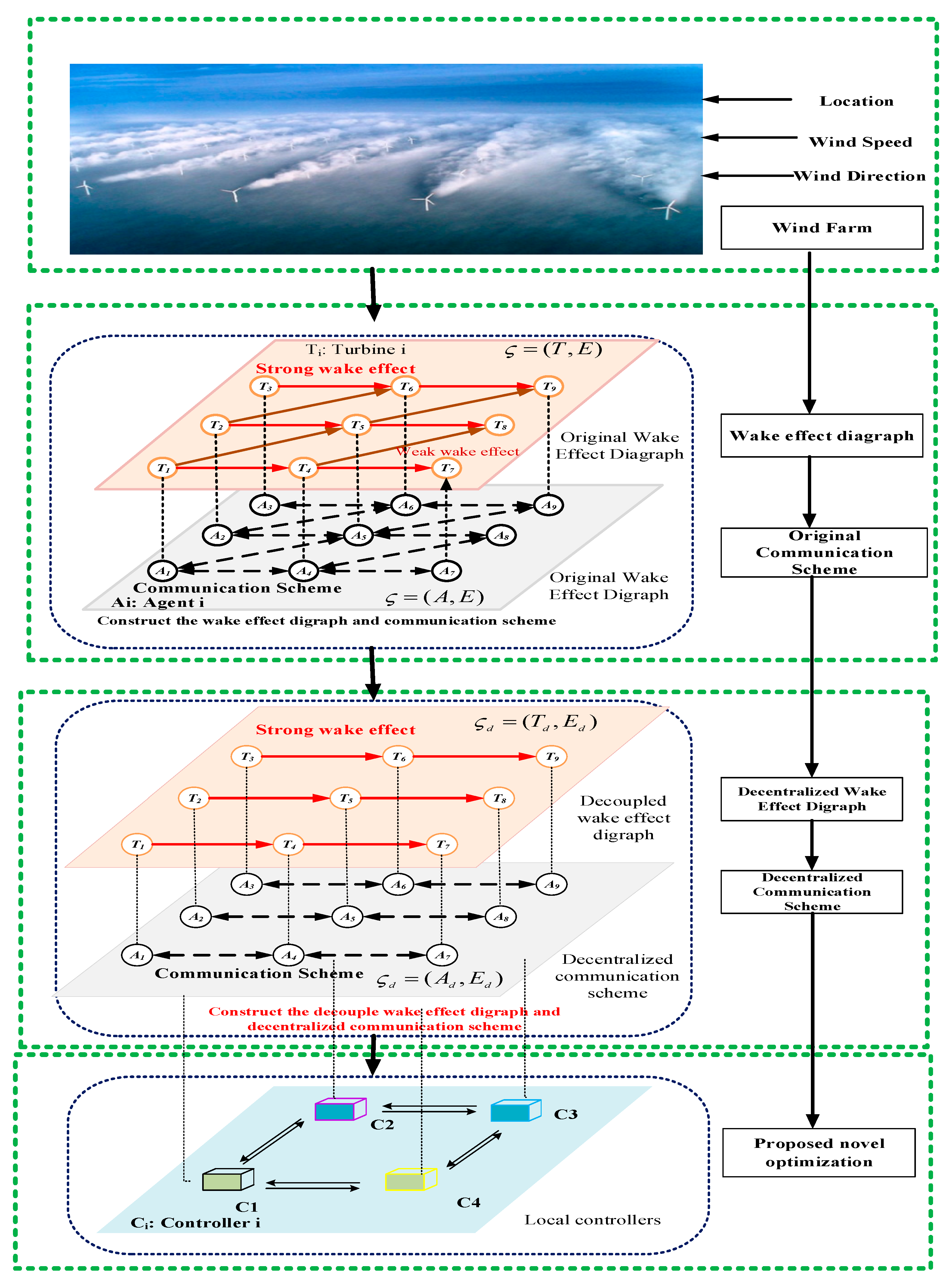
We propose a decentralized communication construction scheme based on a wake-based digraph that can divide a large-scale wind farm into decoupled groups. Every local controller computes the data of turbines in the same group to reduce the communication burden.
(2)
We propose a new multi-objective optimization framework for wind farm profits points, which includes the total output power, the total fatigue load, and the dispatch of the fatigue load on each wind turbine. Our novel method can decrease the maintenance frequency and lower the maintenance cost of the wind farm.
(3)
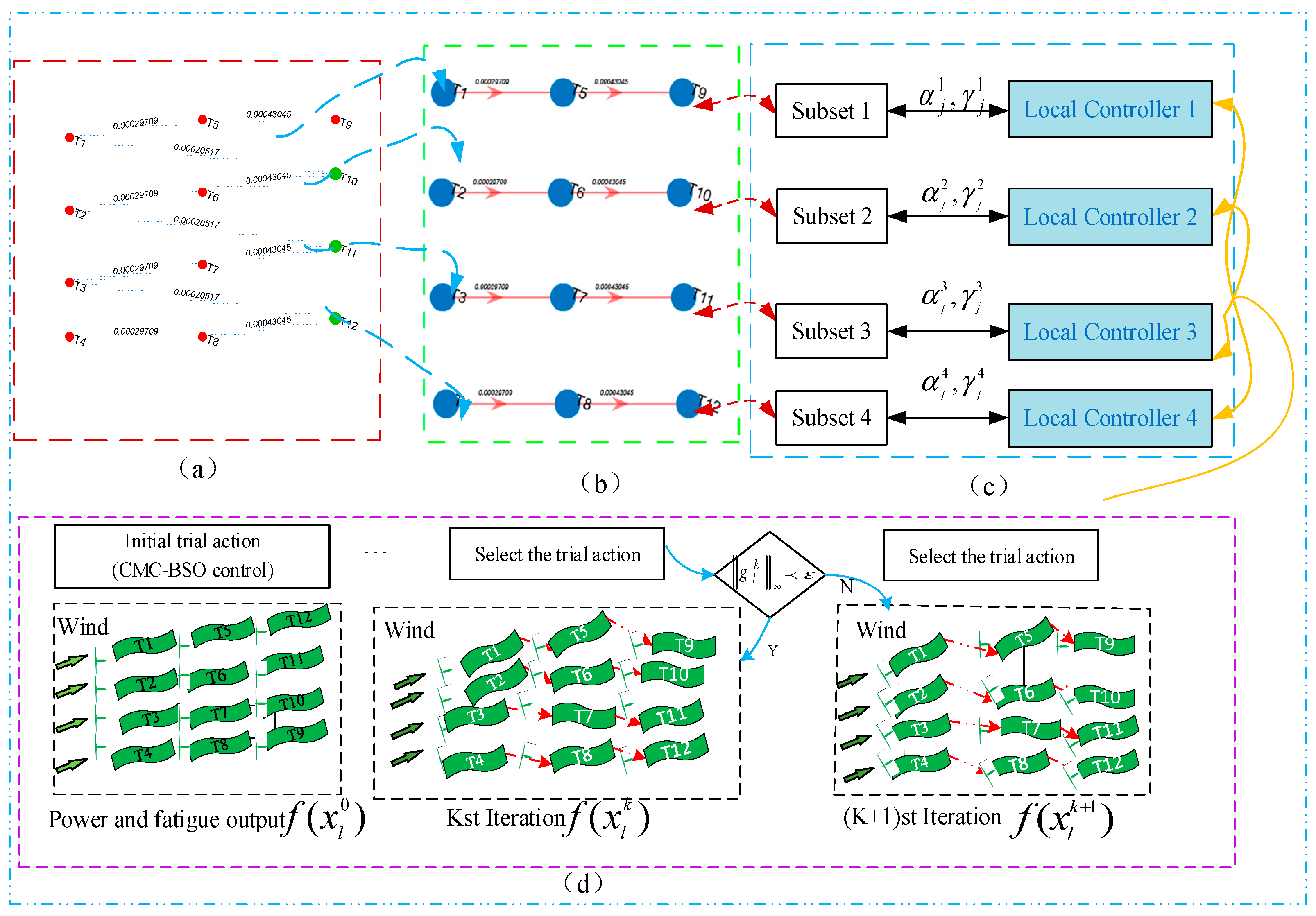
We propose a decentralized CMC-BSO algorithm developed based on a decoupled communication scheme in the wind farm, which combines the advantages of the BSA and PSO algorithms. The algorithm is implemented with a wake steering control to identify the optimized solution on the objectives by controlling the yaw angles and axial factors.
The current paper is organized as follows: Section 2 introduces the wind farm model with wake interactions and its communication system. Section 2 also presents the algorithm, which divides the large-scale OWF into several decoupled subsets. Section 3 presents the novel optimization control strategy utilized to achieve the multi-objects and the simulation result. Finally, the discussion are given in Section 4, and the conclusion and our outline of potential future projects are provided in Section 5.

2. Methodology

This section introduces the new technologies to increase the economic profits of OWF. The road map of this section can be summarized as follows:
As shown in Figure 1, the wind effect wake digraph based on the wind farm model was proposed. Then, a decentralized wake effect digraph and communication scheme is constructed using various practical technologies. Lastly, the local controller for each subset is designed to identify the optimum global value. The specific techniques are illustrated as following:

2.1. Wind Farm Model with Wake Interactions

2.1.1. Wind Turbine Wake Model

This section presents the process of building an OWF power output and fatigue load function based on the Jensen model [31]. To describe the wake effect properties of the upstream turbine T i , the downwind–crosswind coordinate frame ( X i , Y i ) is more suitable than the Cartesian coordinate frame ( X ¯ i , Y ¯ i ) for the characteristic of accuracy with wind variation. The detailed steps are shown as follows:
Firstly, a uniform direction Φ of the free-stream inflow to the wind plant was assumed and averaged the flow direction measurements at the hub of each turbine i , denoted as ϕ i m e a s u r e d :
Φ = 1 N i = 1 N Φ i m e a s u r e d
Secondly, the downwind–crosswind coordinate frame ( X i , Y i ) can be translated from the Cartesian coordinates frame ( X ¯ i , Y ¯ i ) as follows:
[ X i Y i ] = [ c o s ( Φ ) s i n ( Φ ) s i n ( Φ ) c o s ( Φ ) ] [ X ¯ i Y ¯ i ]
The FLORIS model combined with the Jensen model includes wake deficit, wake deflection, and wake expansion model. The three wake zones are defined, each of which has a unique velocity deficit rate, namely, “near wake” (q = 1), “far wake” (q = 2), and “mixed zone” (q = 3). By combining the influence of each wake zone of the upstream turbine T i , the effective speed of the downstream turbine T j can be expressed as:
V j = V [ 1 2 i F : X i < X j α i q = 1 3 c i , q X j , Y j m i n A i , j , q o l A j , 1 2 ]
where V j is the effective inflow wind speed of the turbine T j , V is the undisturbed inflow wind speed of the WF, α i is the axial induction factor of the upstream turbine T i , c i , q ( X j ) is wake zone q velocity deficit factor for T j , A i , j , q o l is the overlapping areas of the q wake zone of upstream T i with downstream turbine T j rotor area, A j is the downstream turbine rotor area. c i , q ( X j , Y j ) is a piecewise wake decay coefficient as follows:
c i , q X i , Y j = c i , 1 X j   when   | d | D w , i , 1 X j / 2 c i , 2 X j   when   D w , i , 1 X j / 2 < | d | D w , i , 2 X j / 2 c i , 3 X j   when   D w , i , 2 X j / 2 < | d | D w , i , 3 X j / 2 0   when   | d | D w , i , 3 X j / 2
d denotes the distance from the wake center to the downstream turbine T j rotor center:
d = Y j y w , i ( X j )
Y w , i ( X j ) is the center dotted line of Y i as shown in Figure 2a, which combines the yaw-induced and rotation-induced wake lateral offsets y w , r o t , i ( X j ) , y w , y a w , i ( X j , V i , a i )   of turbine T j as follow:
y w , i X i = Y i + δ y w , r o t , i X j + δ y w , y a w , i X j , V i , a i δ y w , r o t , i X j = a d + b d X j X i δ y w , y a w , i X j , V i , a i = 0 x x i tan ξ i X j d x ξ i X j = 2 a i 1 a i cos 2 γ i sin γ i 1 + 2 k d X j X i D i 2
In Equation (6), a d and b d denote wake deflection coefficients, ξ i ( X j ) denotes the angle of the centerline of its wake at a downstream location when X j > X i , γ i denotes the yaw angle of the turbine T i , k d denotes the wake deflection coefficients.
The wake decay coefficient c i , q ( X i , X j ) can also be defined as
{ c i , q ( X i , Y j ) = [ D i D i + 2 k e m μ , q ( γ i ) [ X j X i ] ] 2 m μ , q ( γ i ) = M U , q cos ( a μ + b μ γ i )
where D i is the rotor diameter of the turbine T i , k e and m μ , q are the wake expansion coefficients, γ i is yaw angle of the upstream turbine T i , and X j X i is the relative distance between the downstream turbine T j and upstream turbine T i , M U , q , a μ , and b μ are the wake model constants.
The overlapping areas A i , j , q o l , ( q = 1 , 2 , 3 )   between turbines T i and T j rotors and the different downstream zones of the wakes are calculated from the wake center of turbines T i and wake diameter predictions r q using basic geometry as described in Figure 1.
A i , j o l = arccos r q 2 + d 2 R 2 2 · r q · d · r q 2 + arccos R 2 + d 2 r q 2 2 · R · d · R 2 sin arccos r q 2 + d 2 R 2 2 · r q · d · r q · d r q = D W , i , q X j 2 q = 1 , 2 , 3 D w , i , q X j = m a x D i + 2 k e m μ , q γ i X j X i , 0 m μ , q γ i = M U , q cos a μ + b μ γ i
In Equation (8), R denotes the radius of the downstream turbine T j rotor, D W , i , q ( X j ) denotes the diameters of the wake, D i is the diameter rotor of the turbine T i , k e and m μ , q are the wake expansion coefficients, γ i is yaw angle of the upstream turbine T i , and X j X i is the relative distance between the downstream turbine T j and upstream turbine T i . In addition, M U , q , a μ , and b μ are the respective wake model constants.
A large OWF consists of N wind turbines, denoted a set = { 1 , 2 , ,   N } . Combinate Equations (1)–(8), the steady-state electrical power and fatigue loads of a turbine i denoted as P i and F i , are calculated as follows:
P i ( γ i , α i ; V i ) = 1 2 η ρ A i c o s ( γ i ) 1.88 V i 3 4 α i [ 1 α i ] 2
F i ( γ i , α i ; V i ) = 1 2 η ρ A i c o s ( γ i ) 1.88 V i 2 4 α i [ 1 α i ]
where η denotes generator efficiency; ρ denotes the air density; A i denotes the rotor swept area; c o s ( γ i ) 1.88 represent the correction factor added to account for the effects of yaw misalignment [32]; γ i denotes the yaw angle; V i denotes the free-stream wind speed in the front of turbine i ; and α i denotes the axial induction factor. The power production and fatigue loads function can be optimized by adjusting the yaw angles γ i and axial inductions α i , as shown in Equations (9) and (10).

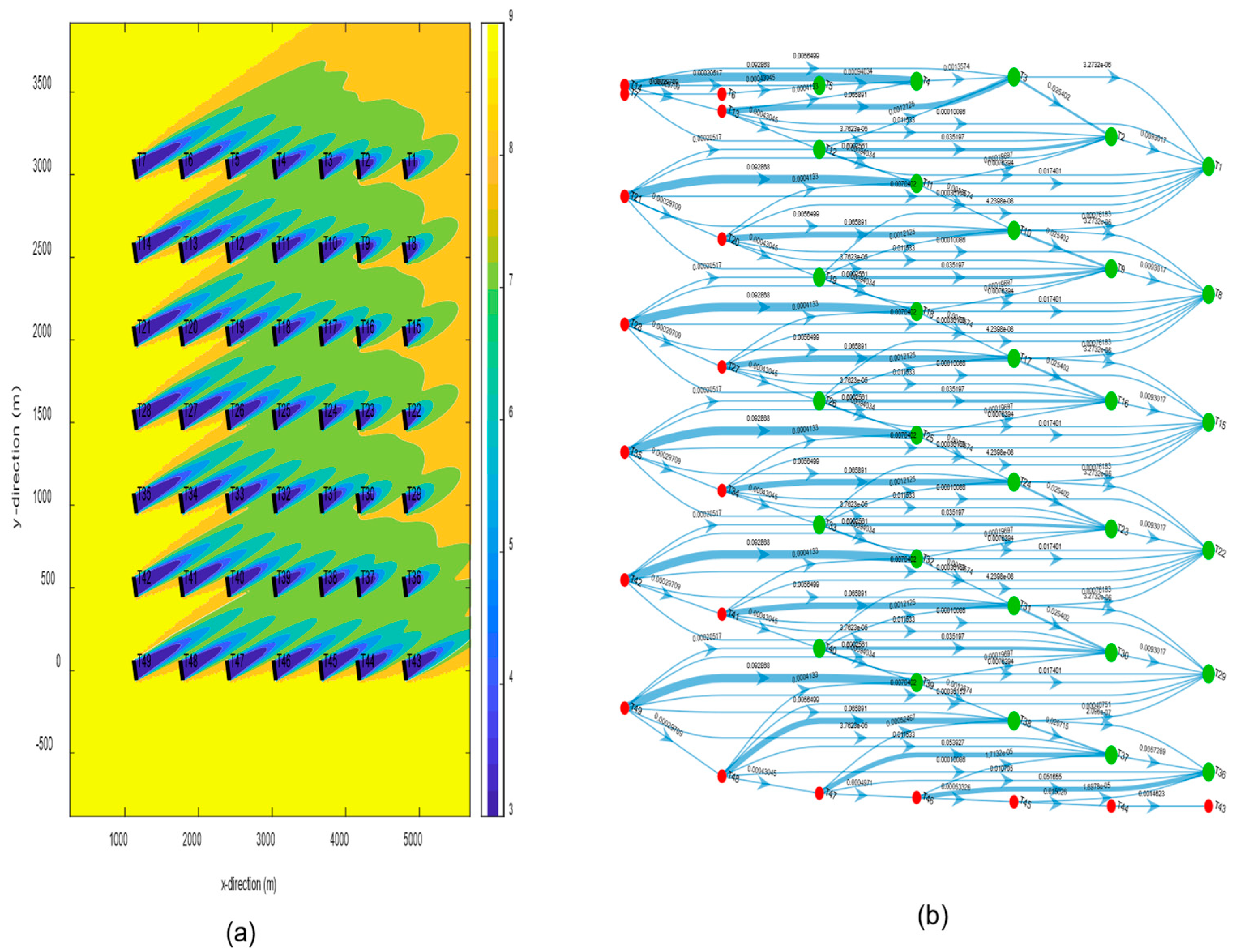
2.1.2. Original Wake Effect Digraph of Offshore Wind Farm

The wake impact on the speed of wind faced by downstream turbines depends on the free-stream wind speed direction Φ and the geographical disposition of turbines ( X ¯ i , Y ¯ i ) within the farm. Therefore, the wake effect faced by some turbines can be either partial or total, as shown in Figure 1. Furthermore, the effect over downstream turbines also depends on the operational conditions of upstream turbines, as stated earlier and it is considered with the induction factor. Nevertheless, the degree of coupling due to wake effects between turbine T i and T j is a function of the wind speed direction as well as the wind farm layout (location and distance among turbines).
As shown in Figure 2b, the wake effect digraph G = (ν, E) of an offshore wind farm can be used to display the relationship between turbines, whereby ν denotes the turbine and E denotes the weight value of the wake effect between every two turbines [19].
E i j = { A i , j o l     V wake   x / D , shadowing 0 , no   shadowing  
where the velocity downstream of the turbine deficit, V wake   = V V j V and the wake overlap effect area, A i , j o l = q = 1 3 A i , j , q o l A j represents the area overlap ratio, which is the wake effect area of the upstream turbine   T i to the downstream turbine j and the rotor area of the downstream turbine   T j (Equation (8)), where x = x j x i represents the physical distance between the upstream turbine T i and downstream turbine   T j ; and D denotes the turbine rotor diameter of all the turbines.

2.2. Decentralized Wake Effect Digraph of Offshore Wind Farm

To decrease the communication information burden, the wake effect digraph needs to construct the decentralized communication topology based on large-scale OWF, as shown in Figure 1. It is essential to identify and divide it into several decoupled groups. In other words, all the wind turbines need to be divided into several decoupled groups based on the wake effect of the OWF, which is performed by the PDFS and HITS algorithms. In this study, in order to identify the network topology of the wake effect directional digraph, the connected turbine with lead turbine T n is found using the PDFS algorithm. It is a clustering algorithm that searches all the node clusters that are centered at the lead turbines by connected edges and then obtains the directed subgraph. However, certain shared nodes inevitably belong to two or more subgraphs, resulting in more iterations and an increased computation time. Therefore, to further decouple the shared turbines based on the subgraph, the HITS algorithm is presented, which focuses on developing ranking algorithms by calculating the authority α i of the input wind and the hub score h i of the output wind based on the shared turbines. As a measure of the authority of shared nodes, we set the value to be larger to correspond to the more important of the wake effect in the subset; we then divided the shared turbine into the subset with the biggest value.
The wake effect digraph is defined as follows: ς = ( ν ,   E ) where nodes ν represent the turbines and E represents the wake interaction strength between any two turbines. Notably, in the wake-based digraph ς, we define the starting nodes (lead turbines) as zero in-degree. The decoupled wake effect digraph is represented as ς d = ( ν d , E d ) , where ν d   and   E d represent the turbines and edges in each decoupled subgraph, respectively.

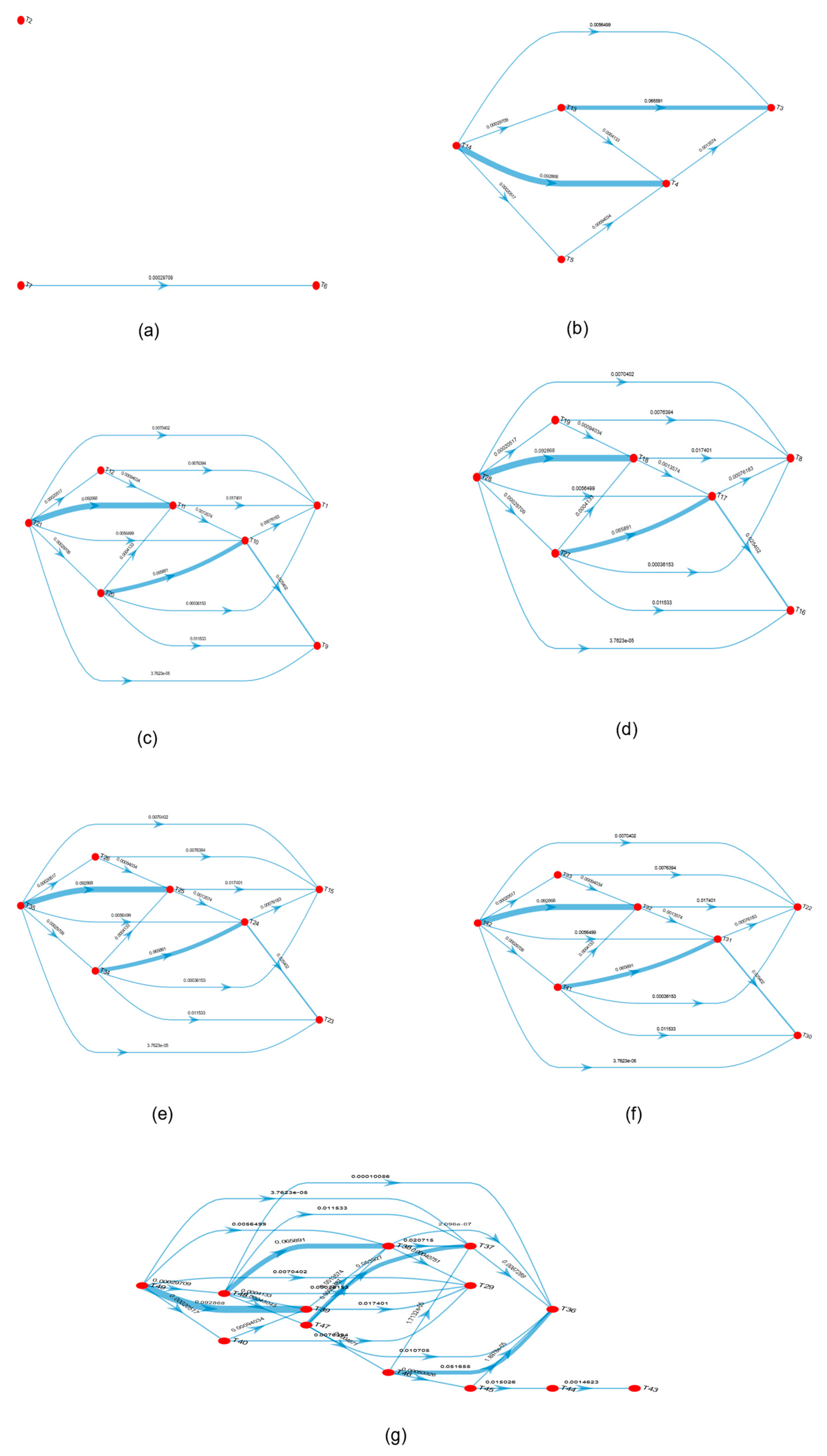
2.2.1. Parallel of Depth-First Search Algorithm to Identify Subgraph

Depth-first Search (DFS) algorithm traversal of the rooted spanning tree τ starting from any turbine r ν produces a spanning tree rooted denoted r, which is known as a DFS tree [33]. The algorithm continue to work from the initial turbine to all reachable turbines and edges.
For a large-scale computationally intensive process in OWF, it is necessary to use the parallel depth-first search (PDFS) algorithm. Before we start the search process, the whole wake digraph needs to be divided into N subsets S N with N local controllers, corresponding to the lead turbines T L , L = {1, 2, … N} Moreover, each controller directs the turbines based on PDFS in the search space. Two key components of the PDFS algorithm are the dividing approach and cutoff depth η. In this paper, considering the relatively low splitting cost factors, the dividing approach divides the whole wake effect digraph into N groups equal to the number of lead turbines T L . In addition, the lead turbines T L are set as the root nodes ν L , and then, the other nodes near them are chosen, especially in situations where the deep degree is huge. Moreover, the cutoff threshold depth η needs to be set as a hyperparameter according to the experience. In this paper, the cutoff threshold depth η was set as η  = D O W F / 2 , with D O W F denoting the depth of the whole wind field.

2.2.2. Calculating the HITS Score of Shared Turbines

In this study, the classical HITS algorithm is used to calculate the HITS score of shared turbines [34]. The main idea of this algorithm is to divide the shared turbines into the group with the maximum authoritative score a i based on the wake effect in OWF.
For the model of the wake effect digraph in an OWF, a i can be defined as the value of one turbine, which is affected by its upstream turbines, and the hubs h i , which can be defined as the effect degree of this node on downstream turbines. However, if we want to construct the decoupled subgraphs, dividing the shared turbines into only the subset with the maximum authoritative value is necessary. Moreover, in this subsection, the HITS algorithm is utilized to calculate the shared authority α i and hub scores h i of the shared turbine and to determine which subgroups they belong to. Algorithm 1 is as follows:
Algorithm 1. The HITS algorithm is based on the wake diagram ς = ( ν ,     E ) .
ν : a collection of v linked turbines
i, c: natural numbers
a 0 = 1 , h 0 = 1
t = 1
do
for each v in ν
do a i ( n ) = ( ν ,     E ) G h i 1 ( ν )
   h i ( n ) = ( ν ,     E ) G a i 1 ( ν )
Normalize: a i = a i a i
Normalize: h i = h i h i
Iteration: i = i + 1
Till α i α i 1 + h i h i 1 < ε
Return ( a i , h i )
Report the nodes with the c largest coordinate in a i .
Report the nodes with the c largest coordinate in h i .
In this study, considering the directional wind effect, the turbines are grouped into the subset with only the maximum authority a i . The original wake digraph ς has a relationship with the wind farm layout ( X , Y ) , wind speed V and wind direction θ . Moreover, the PDFS algorithm can construct the original wake digraph ς. If there are some shared turbines in ς, we can calculate the authorities α i and distribute them into the subset with the largest authority score and then cut off any other corresponding edges.

2.2.3. The Process of Decoupling Shared Turbines Based on the 12-Turbines

In this subsection, we present the process of turbine decoupling through the proposed decoupling strategy. The number of subsets of the turbine groups is determined based on the following: (1) The lead turbine is that whose node authority is zero. In other words, it experiences freestream velocity V . (2) Each lead turbine’s corresponding sub-graph is identified with the PDFS algorithm. (3) The scores of α j and h j in the shared turbines are calculated and compared with each subgraph using the HITS computation algorithm.
From Figure 3, we can see that the original subgraph 1 concludes T1→T10→T5→T9 and subgraph 2 concludes T2→T6→T10→T11, which means turbine T10 is a shared turbine. The reason for this is that the authority score of T10 is 0.0002052 in subset 1 in the subgraph G 1 and 0.0004305 in subset 2 in the subgraph G 2 , respectively, thus T10 is divided into the subgraph G 2 . In addition, other shared turbines T 11 { G 2 , G 3 } and T 12 { G 3 , G 4 } as shown in Figure 3(a_2) are also divided into the subgraph G 3 and G 4 , respectively, as shown in Figure 3d.

2.3. Multi-Objective Optimization Based on Decoupled Groups

In this section, controller design method is presented. To do this, the optimization objective for improving economic profits of the OWF is firstly suggested to increase total power capture, mitigate total fatigue load, and to obtain a more even fatigue distribution than other traditional algorithms. Secondly, the aim of the designer is not only to consider the profits of the whole OWF but also to decrease the fatigue load of an individual turbine, which can reduce the need for replacements and the maintenance cost. Furthermore, the control objectives are reached by identifying the optimization value of the control variables of the axial factor α and yaw-misalignment γ . Finally, an improved CMC-BSO algorithm with the embedded power and fatigue constraints of wind farms is suggested solve the proposed optimization problem, which can guarantee the fast speed necessary for wind farm control.

2.3.1. Formulation of Multi-Objective Optimization

Fatigue is the factor that sustains the stresses with periodical stress characteristics during the process of component damage. The components will slowly deteriorate or even break when there is a large margin of stress variation. This negatively impacts the practical lifetime of the turbines. Therefore, the three-objective function is formulated as follows:
m i n x f ( x ) = i = 1 N j = 1 K ξ P j γ j , α j ; V j + ( 1 ξ ) F j γ j , α j ; V j + σ F j γ j , α j ; V j F t j γ j , α j ; V j δ f F m j γ j , α j ; V j s . t . { γ m i n γ j γ m a x α P _ m i n α Pj α P _ m a x
where F j ( γ j , α j ; V j ) are fatigue load over the whole OWF and F m j ( γ j , α j ; V j ) ,   F t j ( γ j , α j ; V j ) are the fatigue load of each WT from the greedy method and traditional multi-objective optimization approaches [15]. Further, the first two objectives are balanced with hyper-parameter weights ξ . There are also another two hyper-parameters σ and δ F   , σ is used to balance the fluctuation fatigue of individual turbines, and δ F     is the tolerance fluctuation coefficients ratio of the difference fatigue load of the proposed method using the greedy approach [35].
In Equation (12), the three objectives of the optimizations can be summarized as follows: (1) to maximize the available wind power of the OWF at the first part of −ξPj(γj, αj; Vj); (2) to minimize the total fatigue loads of the OWF at the second part of ( 1 ξ ) F j ( γ j , α j ; V j ) ; and (3) to keep the fluctuation of fatigue load within a tolerant value at the third part of σ ( F j ( γ j , α j ; V j ) F t j ( γ j , α j ; V j ) δ f F m j ( γ j , α j ; V j ) ) .

2.3.2. CMC-BSO Optimization Algorithm

In this section, the BAS algorithm is presented to provide less complexity in designing tasks; however, it is not suitable for high-dimensional systems, as has been verified in many experiments [36]. Therefore, to improve its performance, some researchers have proposed the BSO algorithm, which incorporates the main advantage of the swarm optimization algorithm. However, repetitive results have proven not to be stable experimentally because it is more dependent on the initial values. If suitable values are not set, the result has a sub-global optimization value. To solve this problem, the Monte Carlo (MC) law for BSO was introduced to improve the repeatability and stability of the algorithm. This law is to identify the optimized control variables α i and γ i to achieve the multi-objective during the search process. This can be achieved by simulating the annealing process with the random variables in order to escape the local optimized solution.
First of all, various parameter notations are defined by the mathematical formulation as follows: X p = ( X p 1 , X p 2 , , X p n ) T , X g = ( X g 1 , X g 2 , , X g n ) T denotes the position of n   beetles in each turbine and group turbines, X p i = ( X p i 1 , X p i 2 , , X p i L ) T and X g i = ( X g i 1 , X g i 2 , , X g i L ) T denote each beetle with L-dimensional search space, similar to the individual and group beetle speed V p i l = ( V p i 1 , V p i 2 , , V p i L ) T ; V g i l = ( V g i 1 , V g i 2 , , V g i L ) T denotes the best position of each particle P p i l = ( P p i 1 , P p i 2 , , P p i L ) T and the best position of the whole swarm P g i l = ( P g i 1 , P g i 2 , , P g i L ) T [37].
In this study, the CMC-BSO algorithm is presented as follow:
(1)
Update the position on the antennae of individual and group beetles.
The position of beetle i can be represented as follows:
X p i l t + 1 = X p i l t + λ ξ p i l t  
X g i l t + 1 = X g i l t + λ ξ g i l t  
where i = 1 , 2 , , n ; l = 1 , 2 , , L ; The current number of iterations is t   and ξ p i l ; ξ g i l   represents the beetle position movement, and λ is a positive constant weight value.
(2)
Define the movement of beetles.
The   ξ function can be calculated as follows:
ξ p i l t + 1 = ξ p i l t + δ t V p i l t sign f X p r l t f X p l l t
  ξ g i l t + 1 = ξ g i l t + δ t V g i l t sign ( f ( X g r l t ) f ( X g l l t ) )
The step size δ , the beetles’ speed V p i l , V g i l and f ( X p r l t ) ,   f ( X p l l t ) , f ( X g r l t ) ,   and   f ( X g l l t ) are the fitness function of scent intensity at the right and left antennae X p r l t ,   X p l l t , X g r l t ,   X g l l t .
(3)
Define the speed of beetles.
The speed of each beetle and group beetle can be defined according to [38]
V p i l t + 1 = ω V p i l t + c 1 r 1 ( P p i l t X p i l t )
V g i l t + 1 = ω V g i l t + c 1 r 1 ( P p i l t X p i l t ) + c 2 r 2 ( P g i l t X g i l t )
The second part in Equation (17) represents the private thinking of the beetle itself. The third part in Equation (18) represents the collaboration among the beetles. The adaptive inertia weight ω   in Equation (18) varies with the current iterations:
(4)
Define the adaptive inertia weight [39]:
ω = ( ω m i n ω m a x ) t T T + ω m i n
The minimum and maximum values of ω are ω m i n and ω m a x , respectively; these values are set by the respective mean fitness values for the 60 runs. In this study, ω m a x = 0.9 , ω m i n = 0.4 , and c 1 = 0.1 , c 2 = 0.15 . The speed of the beetle has the maximum value when t = T = 1000 and minimum one when t = 0 . Therefore, this can improve the local search speed as compared with the constant value in the traditional BSA method.
(5)
Pre-update the right and left antenna beetles.
The process of updating the position of the right antenna and the left of the individual and group antenna can be expressed by the L-dimension beetles as follows:
X p r l t + 1 = X p r l t + V p i l t d / 2 X p l l t + 1 = X p l l t V p i l t d / 2
X g r l t + 1 = X g r l t + V g i l t d / 2 X g l l t + 1 = X g l l t V g i l t d / 2
where d represents the searching distance which depends on the step size δ as explained in [40].
(6)
Implemented solution of the Monte Carlo law.
The Monte Carlo law is proposed to be embedded into the BSO algorithm to escape the local optimal solutions. The probability is used throughout the iterative process to escape the poorer solutions of individual and group beetles:
L p = { 1 , f ( X i l t + 1 ) < f ( X i l t ) e x p ( f ( X i l t + 1 ) f ( X i l t ) M T ) , f ( X i l t + 1 ) f ( X i l t )
where X i l t + 1   denotes a pre-update position of beetle i ; X i l t   denotes the best position of beetle i in the last iteration; whereas exp (·) represents the exponential function and M T   is the higher temperature.
(7)
Step size:
δ t + 1 = 𝒢 δ t d t = 𝒢 δ t 1 / c 2
where 𝒢 is a constant value that needs to be adjusted by the designer, and in the current study, it was set as 𝒢 = 0.91 .

3. Simulation Results and Discussion

The simulations were carried out based on the OWF, the structure of which is shown in Figure 4. It was implemented with 7 × 7 matrix of the National Renewable Energy Laboratory’s 5 MW turbine in a wind farm with regular shapes.

3.1. Parameter Setup

The wind farm simulation and wake effect simulation data were computed using the FLORIS platform [41]. The longitudinal distance was 5.5 × D, and the lateral distance was also 5.5 × D, as shown in Figure 5. In the present study, we discussed the performance of an OWF with a wind direction range of φ   ϵ   [ 0 ° , 90 ° ] with a   15 ° step size. The initial values in Equation (7) for the yaw angle γ   and the axial factors α were set as 0, 1/3. In addition, the initial value in Equations (15) and (16) for the initial antennae length X p r l t ,   X p l t ,   X g r l t , X g l l t are set as 0.4, 0.5, 0.45, 0.52, respectively. Further, the initial step size δ is set as 1.00, The balance weight was supposed as ξ = 0.5 , and some other hyper-parameters σ = 1.0 , the coefficient tolerant ratio of the fatigue load δ F = 0.03. A series of simulations will be performed in the following subsections.

3.2. Process of Decoupling Groups

The wake field of an OWF with a 7 × 7 matrix is as shown in Figure 5a. The shared turbines are represented as green plots as in Figure 5b. The subgraph of Figure 5b is shown in Figure 6. Figure 6 shows the subgraph of the original wake effect. However, there are shared turbines in each subparagraph. It was necessary to divide the shared turbines into one group. The significant difference between Figure 6 and Figure 7 lies in no shared wind turbines. That is, the share turbine T6 is divided into group 1, and the share turbine T3, T4, and T5 are divided into group 2. The partitioning is depended on the maximum authority score as described in Section 2.2.2. More specific information is shown in Table A1 (Appendix A).

3.3. Optimization Results

The performance of the three objectives under two conditions is examined in this section. One scenario is involved by the wind direction remaining while the wind speed is changed. The other scenario is involved by the wind speed changing while the wind direction remains constant.

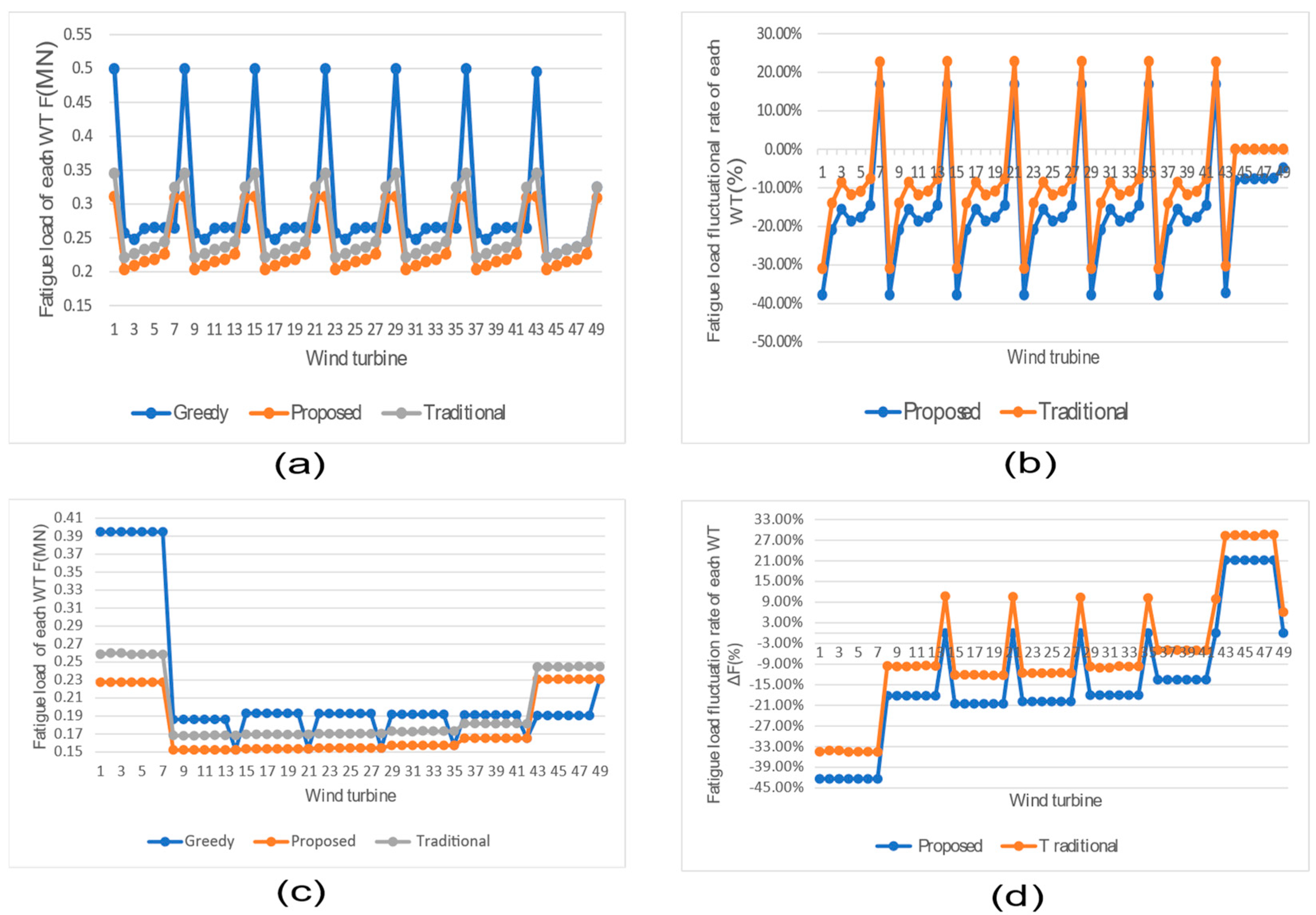
3.3.1. Simulation Results with a Constant Wind Speed

In this subsection, the constant windspeed was set V 0 = 8   m / s and the range of wind direction was φ   ϵ   [ 0 ° , 90 ° ] . The total power output P, fatigue load F, the rate of total power output ΔP, and the rate of total fatigue output ΔF are as shown below:
As shown in Figure 8, there is a proportional relationship between Figure 8a,b, and the negative fluctuation of fatigue load Δ F p r o p o s e d < Δ F t r a d i t i o n l a l verify the advantage of the proposed algorithm as compared with the traditional algorithm. In addition, the minimum value and the maximum values of the output power were φ = 90 ° and φ = 75 ° , respectively. This is because the wake effect has the biggest at φ = 90 ° and the smallest at φ = 75 ° . In addition to the optimization performance of total output power and fatigue load, our novel method results in a more even distribution of fatigue load than the traditional method, which is discussed in the following:
The decoupled subsets at wind direction φ = 0 ° and φ = 90 ° with a wind speed of V 0   ϵ   [ 8   m / s , 11   m / s ] are shown in Table A2 and Table A3 (Appendix A). The total output power and fatigue load were optimized, as shown in Figure 8. In the following, we verify the distribution of fatigue load on individual turbines.
OWF can be divided into seven decoupled subsets corresponding to the lead turbines as T1, T8, T15, T22, T29, T36, and T43. For   F max _ g r e e d y = 0.5   MN , F max _ t r a d i t i o n a l = 0.35   MN , F max _ p r o p o s e d = 0.35   MN , as shown in Figure 9a, it is clear that F max _ p r o p o s e d < F max _ t r a d i t i o n a l < F max _ g r e e d y . In order to explain the improved even distribution of the individual fatigue, the fatigue decrease rate of lead turbine Δ F p r o p o s e d = 30 % > Δ F t r a d i t i o n a l = + 10 % , as shown in Figure 9b. Therefore, the superior performance of the even distribution of the fatigue load is well verified. In addition, when wind direction φ = 90 ° , as shown in Figure 9d, the same conclusion was reached, i.e., Δ F p r o p o s e d = 40 % < Δ F t r a d i t i o n a l = 0 % can be deduced. To achieve the objectives, the control variables of each turbine can identify the optimization value based on the controller, for example, the control. For example, Figure 10 shows the scenario V 0 = 8 m/s φ = 0 ° . As mentioned above, the proposed CMC-BSO algorithm is faster than the MC-BSA algorithm [19]. In this subsection, the reduced computation time and accuracy were verified by comparing other algorithms as shown in the following Table 1, Table 2 and Table 3: Table 1 denotes the computation time, and ΔT denotes the percentage rate of computation time of the other algorithms using the centralized baseline method. In Table 2 and Table 3, P/F denotes the total output power/fatigue load, and ΔPF denotes the increased rate of output power/fatigue load of the other algorithms using the greedy baseline method.
As shown in Table 1, Table 2 and Table 3, various conclusions can be obtained: (1) The proposed algorithm is practical at improving the control speed, i.e., the computation time is the shortest among the four algorithms. (2) For the proposed algorithm, the increase in the output power was not as effective as that of traditional algorithms and centralized algorithms, which means there is a low power cost. (3) For the proposed algorithm, the decrease in the fatigue load was more effective than the other algorithms, as shown in Table 2.

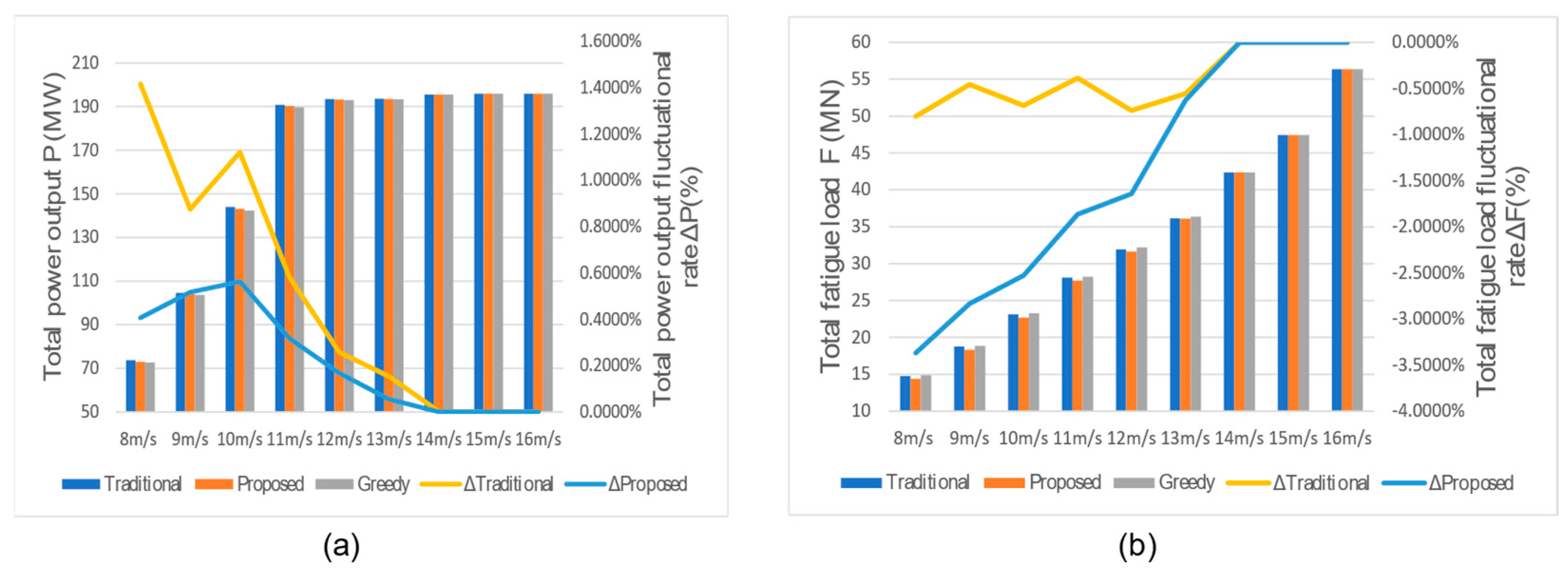
3.3.2. Simulation Results with Constant Wind Directions

As described in the previous subsection, the superior control performance with a constant wind speed of V 0 = 8 m/s is well verified. Furthermore, in this subsection, the control performance is discussed for a scenario of a varying free wind speed of V 0   ϵ   [ 8   m / s ,   16   m / s ] and a constant wind direction of φ = 45 ° .
As shown in Figure 11, with the wind speed of V i < 11.4   m / s , there is a positive correlation between the total output power and the wind speed. When   V i > 11.4   m / s nearly all wind farm turbines produce the rated power, and there are no significant wake losses [42]. However, the fatigue load F increases with the wind speed, as shown in Figure 11b. In this paper, the wake effect is the basic component of an OWF, thus we focused on the performance with V i < 11.4   m / s . The total fatigue load decreased with the proposed algorithm to a greater extent than the traditional algorithms at the cost of a small amount of output power with ΔF.

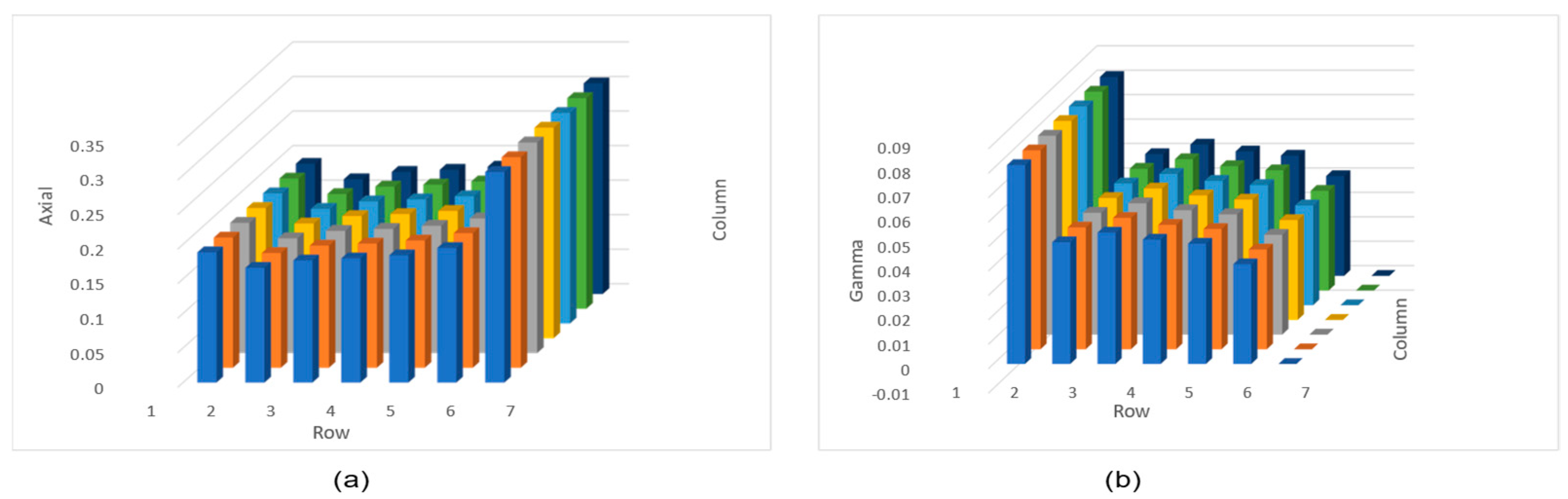
3.3.3. Simulation Results with Different Hyperparameters

This subsection addresses the tuning result with three main hyperparameters: ξ , σ , and δ F   . The wind speed is set at φ = 0 ° , V 0 = 9   m / s by tuning different hyperparameters, and the impaction on the output result can be summarized as follows.
  • The weight value ξ can decide the relationship between P, F, ΔP, and ΔF.
When ξ   varies greater, P and F increase to a greater extent, as is demonstrated in the following tables:
2.
The F , Δ F with a varying hyperparameters value σ.
3.
The F , Δ F with a varying hyperparameters value δ F   .
As shown in Tables 6 and 7, if σ and δ F increase, the fatigue load decrease rate will also increase so that the fatigue load will decrease, which takes the fatigue load decrease ratio of subset 1 ΔFs1.
From the results in Table 4, Table 5, Table 6 and Table 7, the effects of the four hyperparameters can be summarized as follows:
(1)
Weight value ξ is an important weight factor and can be used to adjust the important degree of P or F, and a larger ξ means it is more important to optimize P. If ξ = 0.5 , P and F are optimized at the same degree.
(2)
Hyperparameters values σ and δ F   can affect the fatigue load of each turbine, The greater σ or δ F   , the more the fatigue loads of each subset will decrease (and vice versa). The difference is that hyperparameters δ F   are more sensitive than σ.

4. Discussion

In this section, the effectiveness of the proposed algorithm is discussed compared with different examples:
(1)
The accuracy and control speed of the proposed algorithm. The reaction speed of the proposed algorithm is faster than other methods, and the control time of the CMC-BSO algorithm has been reduced by 9.23% compared to the MC-BAS method in [17] and decreased by 3.98% compared to the traditional multi-objective algorithm in [13] owing to the novel decentralized communication topology.
(2)
The performance of the proposed multi-objective function. With different wind speeds and directions, the implementation of the proposed algorithm compared with the other two methods:
(a)
Compared with the greedy method, the average power output of the proposed algorithm increased by approximately 0.47%. The proposed algorithm demonstrated superior performance regarding fatigue distribution, with an average fatigue decrease rate for the lead turbine of approximately 13.5%. This means the output power has increased, and the fatigue load has decreased.
(b)
Compared with the traditional multi-objective optimization method, the improved performance of the proposed algorithm has also been verified. Although the total output power rate is decreased at 1.5%, the average fatigue decrease rate is 12.3%. Therefore, it can be economically profitable at a low power cost.
(3)
The tuning factors. The different tuning factors of the proposed multi-objective function were analyzed. In this case, the tuning factor ranges from 0.4 to 0.9, and the specific value needs to consider the balance between calculation accuracy and speed.
In the above description, the performance of the proposed method to reach the anticipated objective bears the characteristics of faster speed, increased robustness, and greater accuracy than other methods.

5. Conclusions

This study have proposed a novel three-objective optimization algorithm that utilizes a decentralized framework to address the OWF optimization problem. The performance of the submitted novel algorithm has been verified using a simulation with varying wind speeds and directions. The maximum fatigue load value on the lead turbines can be reduced with the proposed methods. In addition, fatigue load declined to a certain extent for downstream turbines due to wake effect control, and the decrease rate has been lower than that of the traditional method. From a cost point of view, the proposed novel algorithm has been performed well by balancing multiples, although there were some active power losses. The main results of the paper can be summarized as follows:
(1)
The PDFS implemented with the HITS algorithm has been newly proposed in the wake effect digraph of a large-scale OWF, which can be useful for splitting the OWF into decoupled groups. It is of significance and practical importance for us to control the wake effect digraph with a modular and flexible structure.
(2)
A novel multi-objective algorithm has been submitted in this study to increase the economic profits of OWF owners. The importance of this algorithm is of good performance on balancing fatigue load dispatch of each wind turbine on the whole OWF. A quantitative analysis has been conducted comparing the result data of the novel algorithm and the traditional algorithm, and its good performance was well verified.
(3)
It is a non-negligible key technology to design a solver of controllers. The CMC-BSO algorithm has been proposed first in this paper. The practical importance of this paper is to develop a novel control technique by presenting the CMC-BSO algorithm. We have confirmed that it can decrease the probabilities of the suboptimal solution and improve the active speed, which has been verified by comparing the computation time of the MC-BAS algorithm as in Section 3.
However, this paper did not consider wind turbulence and Pareto optimal points, which will be further focused on in future research. In addition, with the growth of large-scale OWF, it is worth developing decoupled group technology to further decrease communication burdens in the field. Moreover, a more accurate high-fidelity CFD model is needed to design the well-optimized performance of the OWF control algorithm [33].

Author Contributions

Conceptualization, Y.C. and Y.H.J.; methodology, Y.C.; software, D.S.; validation, Y.C., D.S. and Y.H.J.; formal analysis, Y.C.; investigation, Y.C.; resources, Y.H.J.; data curation, Y.C.; writing—original draft preparation, Y.C.; writing—review and editing, D.S.; visualization, D.S.; supervision, Y.H.J.; project administration, Y.H.J. All authors have read and agreed to the published version of the manuscript.

Funding

This research was funded by [partially supported by the Basic Science Research Program through the National Research Foundation of Korea (NRF) funded by the Ministry of Education (NRF-2016R1A6A1A03013567, NRF-2021R1A2B5B01001484) and the Innovation-Driven Project of Central South University (2020CX031). The APC was funded by the Basic Science Research Program through the National Research Foundation of Korea (NRF) funded by the Ministry of Education [NRF-2016R1A6A1A03013567, NRF-2021R1A2B5B01001484].

Institutional Review Board Statement

Not applicable.

Informed Consent Statement

Not applicable.

Data Availability Statement

Data sharing is not applicable to this article.

Conflicts of Interest

The authors declare no conflict of interest.

Appendix A

Table A1. Turbine decoupling results and a maximum HITS authority score of shared turbines. (bold font shows the highest score).
SchemeAuthority ScoreDecoupled Subsets
S1:{T7|T6, T5, T4, T3, T2, T1}T6 = 0.013756SD1:{T2|T6, T5, T4, T3, T2}
S2:{T14|T13, T5, T4, T3, T12, T2, T1, T11, T10, T9, T8}T4 = 0.8660
T5 = 0.0019
T13 = 0.0028
T3 = 0.1134
SD2:{T14|T13, T3, T4, T5}
S3:{T21|T20, T19, T10, T9, T8, T18, T17, T16, T15, T11, T1, T12, T3, T2}T1 = 0.0656
T9 = 0.0138
T10 = 0.1049
T11 = 0.8008
SD3:{T21|T12, T11, T10, T1, T20, T9}
S4:{T28|T27, T26, T25, T24, T23, T22, T17, T16, T15, T18, T8, T9, T1, T10, T19}T19 = 0.0018
T18 = 0.8008
T17 = 0.1049
T16 = 0.0138
T8 = 0.0656
SD4:{T28|T19, T18, T17, T16, T27, T8}
S5:{T35|T34, T33, T24, T23, T22, T32, T31, T30, T29, T25, T15, T16, T17, T8, T26}T15 = 0.065594
T23 = 0.013756
T24 = 0.104902
T25 = 0.800807
T26 = 0.001768
SD5:{T35|T26, T25, T24, T23, T34, T15}
S6:{T42|T41, T40, T31, T30, T29, T39, T38, T37, T36, T32, T22, T23, T33, T24, T15}T33 = 0.001768
T32 = 0.800808
T22 = 0.065594
T30 = 0.013756
T31 = 0.104902
SD6:{T42|T33, T32, T22, T31, T41, T30}
S7:{T49|T48, T47, T38, T37, T36, T46, T45, T44, T43, T39, T46, T45, T44, T43, T39}T40 = 0.001758
T39 = 0.796475
T38 = 0.104887
T37 = 0.017292
T29 = 0.065226
T36 = 0.00192
SD7:{T49|T48, T40, T39, T47, T38, T37, T29, T46, T45, T44, T43, T36}
Table A2. Subsets of turbines in a 7 × 7 matrix OWF when the wind direction is φ = 0 ° , V 0   ϵ   [ 8   m / s ,   11   m / s ] .
No. of SubsetsLeadTurbines in Subset
N1T1{T1|T2, T3, T4, T5, T6, T7}
N2T8{T8|T9, T10, T11, T12, T13, T14}
N3T15{T15|T16, T17, T18, T19, T20, T21}
N4T22{T22|T23, T24, T25, T26, T27, T28}
N5T29{T29|T30, T31, T32, T33, T34, T35}
N6T36{T36|T37, T38, T39, T40, T41, T42}
N7T43{T43|T44, T45, T46, T47, T48, T49}
Table A3. Subsets of turbines in a 7 × 7 matrix OWF when the wind direction is φ = 90 ° , V 0   ϵ   [ 8   m / s ,   11   m / s ] .
No. of SubsetsLeadTurbines in Subset
N1T1{T1|T8, T15, T22, T29, T36, T43}
N2T2{T2|T9, T16, T23, T30, T37, T44}
N3T3{T3|T10, T17, T24, T31, T38, T45}
N4T4{T4|T11, T18, T25, T32, T39, T46}
N5T5{T5|T12, T19, T26, T33, T40, T47}
N6T6{T6|T13, T20, T27, T34, T41, T48}
N7T7{T7|T14, T21, T28, T35, T42, T49}

References

  1. Mamouri, A.R.; Khoshnevis, A.B.; Lakzian, E. Experimental study of the effective parameters on the offshore wind turbine’s airfoil in pitching case. Ocean Eng. 2020, 198, 106955. [Google Scholar] [CrossRef]
  2. Song, D.; Li, Z.; Wang, L.; Jin, F.; Huang, C.; Xia, E.; Rizk-Allah, R.M.; Yang, J.; Su, M.; Joo, Y.H. Energy capture efficiency enhancement of wind turbines via stochastic model predictive yaw control based on intelligent scenarios generation. Appl. Energy 2022, 312, 118773. [Google Scholar] [CrossRef]
  3. Song, D.; Tu, Y.; Wang, L.; Jin, F.; Li, Z.; Huang, C.; Xia, E.; Rizk-Allah, R.M.; Yang, J.; Su, M.; et al. Coordinated optimization on energy capture and torque fluctuation of wind turbines via variable weight NMPC with fuzzy regulator. Appl. Energy 2022, 312, 118821. [Google Scholar] [CrossRef]
  4. Rizk-Allah, R.M.; Hassanien, A.E.; Song, D. Chaos-opposition-enhanced slime mould algorithm for minimizing the cost of energy for the wind turbines on high-altitude sites. ISA Trans. 2021, 121, 191–205. [Google Scholar] [CrossRef]
  5. Chen, X.; Huang, L.; Liu, J.; Song, D.; Yang, S. Peak shaving benefit assessment considering the joint operation of nuclear and battery energy storage power stations: Hainan case study. Energy 2021, 239, 121897. [Google Scholar] [CrossRef]
  6. Shafiee, M.; Dinmohammadi, F. An FMEA-Based Risk Assessment Approach for Wind Turbine Systems: A Comparative Study of Onshore and Offshore. Energies 2014, 7, 619–642. [Google Scholar] [CrossRef] [Green Version]
  7. Song, D.; Zheng, S.; Yang, S.; Yang, J.; Dong, M.; Su, M.; Joo, Y.H. Annual Energy Production Estimation for Variable-speed Wind Turbine at High-altitude Site. J. Mod. Power Syst. Clean Energy 2021, 9, 684–687. [Google Scholar] [CrossRef]
  8. Perveen, R.; Kishor, N.; Mohanty, S.R. Off-shore wind farm development: Present status and challenges. Renew. Sustain. Energy Rev. 2014, 29, 780–792. [Google Scholar] [CrossRef]
  9. Liao, H.; Hu, W.; Wu, X.; Wang, N.; Liu, Z.; Huang, Q.; Chen, C.; Chen, Z. Active power dispatch optimization for offshore wind farms considering fatigue distribution. Renew. Energy 2020, 151, 1173–1185. [Google Scholar] [CrossRef]
  10. Ahmad, T.; Basit, A.; Anwar, J.; Coupiac, O.; Kazemtabrizi, B.; Matthews, P.C. Fast Processing Intelligent Wind Farm Controller for Production Maximisation. Energies 2019, 12, 544. [Google Scholar] [CrossRef] [Green Version]
  11. Knudsen, T.; Bak, T.; Svenstrup, M. Survey of wind farm control-power and fatigue optimization: Survey of wind farm control. Wind Energy 2015, 18, 1333–1351. [Google Scholar] [CrossRef]
  12. Zhao, H.; Wu, Q.; Guo, Q.; Sun, H.; Xue, Y. Distributed Model Predictive Control of a Wind Farm for Optimal Active Power ControlPart II: Implementation With Clustering-Based Piece-Wise Affine Wind Turbine Model. IEEE Trans. Sustain. Energy 2015, 6, 840–849. [Google Scholar] [CrossRef] [Green Version]
  13. Baros, S.; Ilic, M.D. Distributed Torque Control of Deloaded Wind DFIGs for Wind Farm Power Output Regulation. IEEE Trans. Power Syst. 2017, 32, 4590–4599. [Google Scholar] [CrossRef]
  14. Zhong, S.; Wang, X. Decentralized Model-Free Wind Farm Control via Discrete Adaptive Filtering Methods. IEEE Trans. Smart Grid 2018, 9, 2529–2540. [Google Scholar] [CrossRef]
  15. Shu, T.; Song, D.; Joo, Y.H. Decentralised optimisation for large offshore wind farms using a sparsified wake directed graph. Appl. Energy 2021, 306, 117986. [Google Scholar] [CrossRef]
  16. Ghosh, S.; Senroy, N. Balanced truncation based reduced order modeling of wind farm. Int. J. Electr. Power Energy Syst. 2013, 53, 649–655. [Google Scholar] [CrossRef]
  17. Pulgar-Painemal, H.A.; Sauer, P.W. Towards a wind farm reduced-order model. Electr. Power Syst. Res. 2011, 81, 1688–1695. [Google Scholar] [CrossRef]
  18. Huang, S.; Wu, Q.; Guo, Y.; Lin, Z. Bi-level decentralized active and reactive power control for large-scale wind farm cluster. Int. J. Electr. Power Energy Syst. 2019, 111, 201–215. [Google Scholar] [CrossRef]
  19. Chen, Y.; Joo, Y.H.; Song, D. Modified Beetle Annealing Search (BAS) Optimization Strategy for Maxing Wind Farm Power through an Adaptive Wake Digrah Clustering Approach. Energies 2021, 14, 7326. [Google Scholar] [CrossRef]
  20. Roque, P.; Chowdhury, S.; Huan, Z. Performance Enhancement of Proposed Namaacha Wind Farm by Minimising Losses Due to the Wake Effect: A Mozambican Case Study. Energies 2021, 14, 4291. [Google Scholar] [CrossRef]
  21. Yang, J.; Wang, L.; Song, D.; Huang, C.; Huang, L.; Wang, J. Incorporating environmental impacts into zero-point shifting diagnosis of wind turbines yaw angle. Energy 2021, 238, 121762. [Google Scholar] [CrossRef]
  22. Zhao, R.; Shen, W.; Knudsen, T.; Bak, T. Fatigue distribution optimization for offshore wind farms using intelligent agent control: Fatigue distribution optimization for offshore wind farms. Wind Energy 2012, 15, 927–944. [Google Scholar] [CrossRef] [Green Version]
  23. Kanev, S.; Bot, E.; Giles, J. Wind Farm Loads under Wake Redirection Control. Energies 2020, 13, 4088. [Google Scholar] [CrossRef]
  24. Zhang, B.; Soltani, M.; Hu, W.; Hou, P.; Chen, Z. A wind farm active power dispatch strategy for fatigue load reduction. In Proceedings of the 2016 American Control Conference (ACC), Boston, MA, USA, 6–8 July 2016; pp. 5879–5884. [Google Scholar]
  25. Bossanyi, E. Combining induction control and wake steering for wind farm energy and fatigue loads optimisation. J. Phys. Conf. Ser. 2018, 1037, 032011. [Google Scholar] [CrossRef] [Green Version]
  26. Yuan, Y.; Tang, J. On Advanced Control Methods toward Power Capture and Load Mitigation in Wind Turbines. Engineering 2017, 3, 494–503. [Google Scholar] [CrossRef]
  27. Kirchner-Bossi, N.; Porté-Agel, F. Wind Farm Area Shape Optimization Using Newly Developed Multi-Objective Evolutionary Algorithms. Energies 2021, 14, 4185. [Google Scholar] [CrossRef]
  28. Lv, J.; Sun, W.; Wang, H.; Zhang, F. Coordinated Approach Fusing RCMDE and Sparrow Search Algorithm-Based SVM for Fault Diagnosis of Rolling Bearings. Sensors 2021, 21, 5297. [Google Scholar] [CrossRef]
  29. Hasager, C.B.; Rasmussen, L.; Peña, A.; Jensen, L.E.; Réthoré, P.-E. Wind Farm Wake: The Horns Rev Photo Case. Energies 2013, 6, 696–716. [Google Scholar] [CrossRef]
  30. Chanfreut, P.; Maestre, J.M.; Camacho, E.F. A survey on clustering methods for distributed and networked control systems. Annu. Rev. Control 2021, 52, 75–90. [Google Scholar] [CrossRef]
  31. Sizhuang, L.; Youtong, F. Analysis of the Jensen’s model, the Frandsen’s model and their Gaussian variations. In Proceedings of the 2014 17th International Conference on Electrical Machines and Systems (ICEMS), Hangzhou, China, 22–25 October 2014; pp. 3213–3219. [Google Scholar]
  32. Gebraad, P.M.O.; Teeuwisse, F.W.; van Wingerden, J.W.; Fleming, P.A.; Ruben, S.D.; Marden, J.R.; Pao, L.Y. Wind plant power optimization through yaw control using a parametric model for wake effects—A CFD simulation study: Wind plant optimization by yaw control using a parametric wake model. Wind Energy 2016, 19, 95–114. [Google Scholar] [CrossRef]
  33. Ghaffari, M.; Parter, M. Near-Optimal Distributed DFS in Planar Graphs 16. In Proceedings of the 31st International Symposium on Distributed Computing, DISC 2017, Vienna, Austria, 16–20 October 2017. [Google Scholar] [CrossRef]
  34. Kleinberg, J.M. Authoritative sources in a hyperlinked environment. J. ACM 1999, 46, 604–632. [Google Scholar] [CrossRef]
  35. Park, J.; Kwon, S.; Law, K.H. Wind farm power maximization based on a cooperative static game approach. SPIE Proc. 2013, 8688, 204–218. [Google Scholar]
  36. Jiang, X.; Li, S. BAS: Beetle Antennae Search Algorithm for Optimization Problems. 2017. Available online: http://arxiv.org/abs/1710.10724 (accessed on 10 February 2022).
  37. Shi, Y.; Eberhart, R. A Modified Particle Swarm Optimizer. In Proceedings of the 1998 IEEE International Conference on Evolutionary Computation Proceedings. IEEE World Congress on Computational Intelligence (Cat. No. 98TH8360), Anchorage, AK, USA, 4–9 May 1998; pp. 69–73. [Google Scholar] [CrossRef]
  38. Poli, R.; Kennedy, J.; Blackwell, T. Particle swarm optimization: An overview. Swarm Intell. 2007, 1, 33–57. [Google Scholar] [CrossRef]
  39. Wu, Z.; Zhou, J. A Self-Adaptive Particle Swarm Optimization Algorithm with Individual Coefficients Adjustment. In Proceedings of the 2007 International Conference on Computational Intelligence and Security (CIS 2007), Harbin, China, 15–19 December 2007; pp. 133–136. [Google Scholar] [CrossRef]
  40. Jiang, X.; Li, S. Beetle antennae search without parameter tuning (BAS-WPT) for multi-objective optimization. Filomat 2020, 34, 5113–5119. [Google Scholar] [CrossRef]
  41. FLORIS. Data-Driven Control (TU Delft). Available online: https://github.com/TUDelft-DataDrivenControl/FLORISSE_M (accessed on 13 February 2022).
  42. Howland, M.F.; Dabiri, J.O. Wind Farm Modeling with Interpretable Physics-Informed Machine Learning. Energies 2019, 12, 2716. [Google Scholar] [CrossRef] [Green Version]
Figure 1. Decentralized multi-objective optimization framework in a large-scale wind farm [29,30].
Energies 15 02336 g001
Figure 2. Three different wake zones of wind model. (a) the wake zones behind the turbine Ti. (b) the overlap zones between turbine Ti and turbine Tj [32].
Energies 15 02336 g002
Figure 3. The process used for the 12-turbine decoupled group subset; (a) wakefield and wake-based digraph 𝒢; (b) 4 original subset; (c) the authorities value of 3 shared turbines; (d) 4 decoupled subset 𝒢d.
Energies 15 02336 g003
Figure 4. The framework for the decentralized optimization algorithm based on the wake effect digraph of OWF; (a) wakefield and wake effect digraph; (b) decoupled groups (c) the local controller for each subset; (d) the CMC-BSO algorithm.
Energies 15 02336 g004
Figure 5. Wakefield of OWF when φ, V0 = 8 m/s: (a) 7 × 7 turbines wake field; (b) 7 × 7 turbines original wake digraph.
Energies 15 02336 g005
Figure 6. The subgraph of the seven original wake effect subgraphs: (a) subset 1; (b) subset 2; (c) subset 3; (d) subset 4; (e) subset 5; (f) subset 6; (g) subset 7.
Energies 15 02336 g006
Figure 7. The subgraph of the seven decoupled wake effect subgraph: (a) subset 1; (b) subset 2; (c) subset 3; (d) subset 4; (e) subset 5; (f) subset 6; (g) subset 7.
Energies 15 02336 g007
Figure 8. (a) Fluctuational rate of the power output (b) Fluctuational total fatigue load.
Energies 15 02336 g008
Figure 9. Power output and fatigue load of each WT at a constant wind speed of V0 = 8 m/s: (a) fatigue load F with φ = 0°; (b) fatigue fluctuation rate ΔF with φ = 0°; (c) fatigue load F with a wind direction of φ = 90°; (d) fatigue fluctuation rate ΔF with φ = 90°.
Energies 15 02336 g009
Figure 10. The control variables with wind speed V0 = 8 m/s and wind direction φ = 0°: (a) the axial induction factors ai of each turbines; (b) the yaw angles γi of each turbines.
Energies 15 02336 g010
Figure 11. Total output power and fatigue load with varying wind speed: (a) total power output with wind direction; (b) total fatigue load with wind direction.
Energies 15 02336 g011
Table 1. Comparison of the computation time with V 0 = 8   m / s , φ   ϵ   [0°, 90°].
φ T Algorithm (s)ΔT of Decentralized Algorithm
CentralizedCMBSAProposedTraditional
4129.417.69%7.22%7.39%
15°3678.358.32%7.57%7.92%
30°3195.169.06%8.41%8.61%
45°3579.487.69%6.93%7.02%
60°2889.579.06%8.02%8.59%
75°2849.798.29%7.08%7.71%
90°2708.917.67%7.11%7.37%
Average23,030.678.23%7.47%7.78%
Table 2. Comparison of the total fatigue load of several algorithms with V 0 = 8   m / s , φ   ϵ   [0°, 90°].
F BaselineΔF of Algorithm (s)ΔF of Decentralized Algorithm
GreedyCentralizedProposedTraditional
10.62247.43%1.36%3.86%
15°15.71246.42%1.16%4.97%
30°16.00095.40%0.66%3.39%
45°14.17185.94%1.40%4.10%
60°14.73165.36%1.31%3.87%
75°16.38645.54%1.30%3.89%
90°10.00348.90%1.75%4.26%
Average97.62896.24%1.24%4.04%
Table 3. Comparison of the total output power of several algorithms with V 0 = 8   m / s , φ   ϵ   [0°, 90°].
P Baseline ΔP of the Centralized (s) ΔP of Decentralized Algorithm
GreedyAlgorithmProposedTraditional
48.8774.50%1.68%2.70%
15°83.78461.58%0.01%0.88%
30°84.14321.43%0.07%0.79%
45°72.63991.86%0.41%1.42%
60°76.45261.82%0.10%0.88%
75°87.55581.03%0.19%0.79%
90°45.38923.51%2.06%3.10%
Average71.2631862.00%0.47%1.31%
Table 4. The total power output with a varying weight value ξ .
Weight   Value   ξ P_Greedy (W)P_Novel Algorithm (W)ΔP
0.269,070,174.6472,914,910.216%
0.369,768,511.9377,803,254.8712%
0.469,913,115.7678,815,630.6513%
0.567,947,71179,137,971.216%
0.667,947,71179,137,971.217%
0.767,947,71179,922,278.418%
0.868,429,385.382,338,785.520%
0.968,429,385.384,357,546.723%
Table 5. The F , Δ F with varying weight value ξ .
Weight   Value   ξ F_Greedy (N)F_Novel Algorithm (N)ΔF
0.213,884,399.210,530,049.5−24%
0.314,443,457.512,042,756.6−17%
0.414,443,457.512,518,335.6−13%
0.514,443,457.512,822,310.3−11%
0.614,232,568.412,967,260.6−10%
0.714,443,457.513,050,097.4−9%
0.814,253,567.513,948,030.2−2%
0.913,167,647.113,113,747.10%
Table 6. Subset 1 of each turbine fatigue fluctuation rate with varying σ .
σ ΔFT1ΔFT2ΔFT3ΔFT4ΔFT5ΔFT6ΔFT7ΔFS1
00%−14%−9%−12%−11%−8%23%−11%
0.1−32%−15%−9%−13%−12%−8%22%−12%
0.2−32%−15%−10%−13%−12%−9%22%−13%
0.3−33%−16%−11%−14%−13%−10%21%−13%
0.4−34%−17%−12%−15%−14%−11%20%−14%
0.5−35%−18%−13%−16%−15%−12%20%−15%
0.6−36%−19%−14%−17%−16%−12%19%−16%
0.7−37%−20%−15%−18%−17%−13%18%−17%
0.8−38%−21%−16%−19%−18%−15%17%−18%
0.9−39%−22%−17%−20%−19%−16%16%−19%
Table 7. Subset 1 of each turbine fatigue fluctuation rate with varying δ F .
δ F     ΔFT1ΔFT2ΔFT3ΔFT4ΔFT5ΔFT6ΔFT7ΔFS1
0.04−21%−8%−7%−3%−6%−2%21%−6%
0.05−24%−9%−7%−3%−6%−4%19%−7%
0.06−25%−10%−9%−4%−8%−9%18%−9%
0.07−27%−12%−10%−8%−9%−9%18%−10%
0.08−33%−16%−11%−14%−13%−10%21%−13%
0.09−34%−17%−11%−15%−14%−11%22%−14%
0.1−34%−17%−11%−15%−17%−14%21%−14%
0.12−35%−18%−15%−18%−21%−14%21%−16%
0.13−35%−19%−15%−19%−21%−14%21%−17%
0.14−36%−20%−16%−19%−22%−15%19%−18%
0.15−36%−24%−23%−22%−24%−17%19%−20%
Publisher’s Note: MDPI stays neutral with regard to jurisdictional claims in published maps and institutional affiliations.

