Abstract
Bathymetric surveys performed using small, unmanned vessels are increasingly used in coastal areas and regions difficult to access by hydrographic motorboats. Their geometric dimensions, manoeuvring parameters, low labour intensity, and costs of survey execution have allowed the unmanned survey vessel (USV) to be a commonly recognised surveying platform. It is equipped with a navigation system for positioning, maintaining a course or survey line, determining spatial orientation, and measuring depths. The operation zone of the global navigation satellite system (GNSS) in coastal water regions enables geodetic positioning in land-based surveys and of moving objects, also including, for example, a sounding vessel. Under difficult observational conditions, the positioning is limited by the obscuration of the upper hemisphere, i.e., the visibility of satellites and the reflection from high field buildings. This poses a threat to a small vessel operating at a very short distance from a hydro-engineering structure. Based on a study performed in a marina, the article presents the determination of the minimum safe distance of the planned survey line to the quay in terms of the USV’s dimensions under good sounding conditions. These include low and constant velocity and good observational conditions for a GNSS receiver. The analysis was conducted on survey lines perpendicular to the quay, which was approached twice at distances of 1–5 m, with a 0.5 m interval. A 1 m distance between the end of the survey line and the quay has been determined for the safety of USV’s navigation and continuity of geospatial data collection during bathymetric surveys.
1. Introduction
Modern geospatial surveys, i.e., both photogrammetric surveys by unmanned aerial vehicles (UAVs) [1,2,3,4,5,6,7] and bathymetric surveys by unmanned survey vessels (USVs) [8,9,10,11,12,13], are increasingly performed using unmanned vessels. As dynamic units, they move along a fixed trajectory, thus ensuring data coverage of an area in a manner appropriate to the method, i.e., with photographs or geospatial data. The coverage can be 100%, 200% or 400% [14,15,16,17,18,19,20] when acquiring a wide swatch [21,22,23,24].
Bathymetric surveys intended to obtain information on the bottom shape use hydroacoustic devices: single-beam echosounders (SBES) and multibeam echosounders (MBES). Unmanned surface vessels (USVs) are increasingly used, particularly in the littoral zone and in harbour basins. They differ in hull design and propulsion system and include single- and double-hull vessels fitted with a propeller, or are propeller-less.
One of the most important roles of USVs are hydrographic measurements: port basins, lakes, rivers and small reservoirs, whose aim is to measure the seafloor relief with the appropriate accuracy. In addition, USVs are increasingly used for tasks related to supporting the navigation process [25], in underwater photogrammetry [26], or in geological works [27].
The widespread application of MBES has not pushed the hydrographic SBES from the market [28,29,30]. When sounding using the SBES, the depth measurements are taken vertically under the echo sounder, and it is required to keep an appropriate distance between survey lines, usually no longer than the determined distance. This is why it is crucial for the USV to maintain the survey line. This can be ensured by the operator’s experience in manual mode or by the steering algorithm (autopilot) in automatic mode.
The navigation safety of an unmanned vessel is high under open = space conditions. Both an aerial vehicle operating in an undeveloped and non-forested area and a vessel operating in open water can safely carry out a surveying campaign. The safety of a vessel decreases (or is even jeopardised) when a UAV is to perform a survey in an urbanised area, between buildings, or under a bridge or viaduct. The observational conditions for determining the GNSS position coordinates are difficult [31,32,33], reducing positioning accuracy.
Bathymetric surveys are jeopardised by high harbour structures, which hinder the positioning using a single- (GPS—global positioning system) or dual-system (GPS/ GLONASS—globalnaja nawigacionnaja sputnikowaja sistiema) GNSS receiver [34,35,36,37,38,39,40,41,42,43,44]. Other factors that hinder bathymetric surveys in a restricted water region include quays, breakwaters, moored vessels (in harbours and shipyards) and floating platforms in marinas. Both UAVs and USVs are at risk of being destroyed in a collision with another object.
Bathymetric (sounding) surveys are the basic type of hydrographic work performed for navigation safety purposes, primarily for marine cartography, i.e., map editing and nautical publications. According to the level of detail, the following sounding work types are distinguished: systematic sounding and check sounding. During systematic sounding, the surveyed water region is covered with a system (network) of basic and control survey lines, with a pre-set survey frequency and accuracy. This is the basic type of sounding work for navigation safety purposes. The level of detail and the required accuracy are determined according to the surveyed water region category [14,15,16,17,18]. Check sounding is also performed along a specified network of survey lines with a level of detail different than that for systematic sounding, with the intention to check the reliability of the previously performed systematic sounding or to preliminarily determine the degree of changes that have occurred in the bathymetry of the water region [19,20].
The main stage of the works involves measuring and recording the surveyed parameters (the depths of corresponding positions and all accompanying elements) in a fixed format and with a specified frequency on planned survey lines (points) in accordance with the adopted methodology. The arrangement of survey lines is planned according to the water region and the type of hydroacoustic device for depth measurement or bottom cleanliness investigation. For SBES, MBES, and SSS (side-scan sonar) surveys, the survey lines are planned differently. This article focuses on the use of SBES (which the USV used for bathymetric surveys of the marina in Puck is equipped with).
Bathymetric surveys using a USV equipped with SBES are performed in an arrangement of parallel survey lines at specified distances between each other, parallel or perpendicular to a hydro-engineering structure [45,46]. The first survey should be performed at the shortest distance to the structure. With the GNSS receiver antenna installed at the geometric centre of the USV (horizontally, halfway between the left and right side, and between the bow and the stern), the first survey will be performed further than half of its width in the arrangement of survey lines parallel to the structure. In an arrangement perpendicular to the structure, the distance of the first survey will be longer than half of the length (or the distance between the GNSS antenna and the bow). Additionally, both the error of coordinate determination by GNSS receiver and manoeuvring parameters and hydrometeorological conditions need to be taken into account. It is therefore important to keep the USV precisely on the line at a very short distance from the quay.
One of the navigation parameters determined during route navigation (in hydrography during navigation along a line) is the cross-track error XTE [47,48,49,50]. It is determined in a hydrographic system based on the coordinates of the survey line’s start and end and the current position of the GNSS antenna as the distance between the point and the straight line. It is also used in the automatic navigation process using an autopilot. Thanks to the autopilot, its optimally selected parameters and the data acquired from external sensors, the USV is expected to move along the survey lines optimally, i.e., with a pre-determined velocity and the minimum XTE value.
The article stems from the experience gained in hydrographic surveys in hard-to-reach (restricted) water regions under different GNSS observational conditions: good (open upper hemisphere and good visibility of satellites) and hard (areas with high infrastructure and close to vessels with restricted visibility of satellites and signals reflections).
The article is structured as follows. Section 2 presents the surveyed water region and the surveying vessel used in the study. It also characterises the USV’s circulation radius when changing survey lines and autopilot as the steering system in the automatic navigation mode. Section 3 presents the USV’s trajectory on four survey lines perpendicular to the quay, whose distance to the quay decreases from 5 to 1 m with intervals of 0.5 m. The following navigation parameters were analysed: XTE, the course, and the velocity on turns onto the next survey line from the quayside. Section 4 presents an analytical geometric circulation radius and the angular velocity of the USV. The analysis was conducted in terms of the approach to the quay and the circulation radius size.
2. Materials and Methods
2.1. Study Area
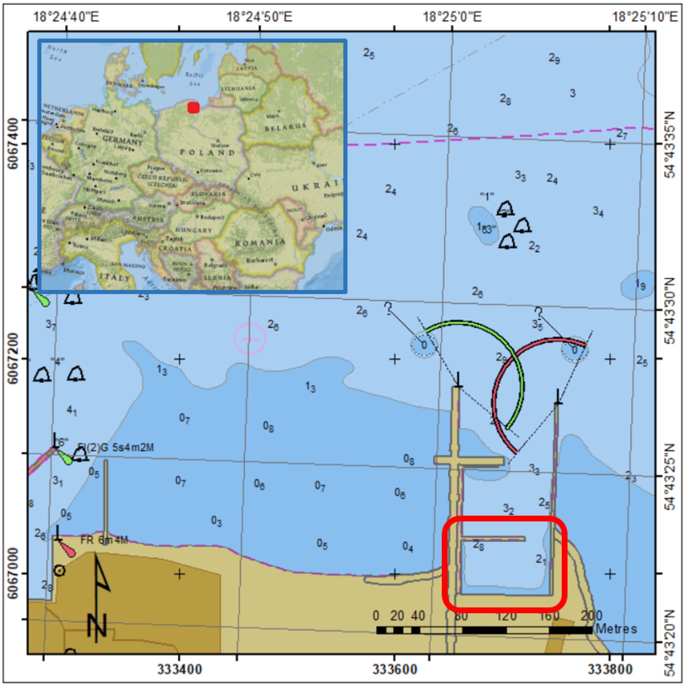
Puck Harbour is located on the western coast of Puck Bay in the Kaszuby Coastal Region, Poland. It comprises two harbour basins: a fishing basin and a marina basin. The marina in Puck accommodates vessels with a hull length of up to 20 m and a draught of up to 2.8 m. The marina is flanked by a 190 m-long pier from the west and a 180 m-long eastern breakwater. There is a 30 m-wide entrance to the marina. The depths are 1.5–3.5 m on the approach and 0.7–3.5 m in the basin. Surveys of the USV’s safe manoeuvring limit in a restricted water region were performed in the southern basin are indicated in Figure 1 and were prepared based on ENC PL5PPUCK.
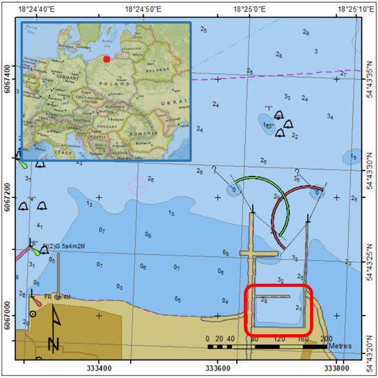
Figure 1.
Puck Harbour with the area of research.
2.2. Methodology for Planning Surveys in a Restricted Water Region
In coastal water regions, the basic survey lines are designed perpendicular to the bottom relief course, the general direction of the isobaths, or the coastline. Control lines are designed perpendicular to the basic lines. In marine hydro-engineering structures, the basic lines are designed parallel to the course of the hydro-engineering structure [19,20].
A reduction in the size of a sounding vessel (replacing hydrographic motorboats with USVs) enables the performance of bathymetric surveys in very restricted water regions. The performance of a sounding becomes easier thanks to greater manoeuvrability, which enables starting a line and ending it near a hydro-engineering structure. The surveys are performed more quickly, which enables the densification of survey profiles (reducing the distance between the lines from 5–10 m for a sounding performed using a hydrographic motorboat to 2 m, or even 1 m for a sounding performed using a USV) [51,52,53].
2.3. Survey Platform—USV Ocean Alfa SL20
An OceanAlpha SL20 USV (Figure 2) is a hydrographic vessel equipped with an SBES Echologger and an internal GPS receiver, which is usually replaced with a geodetic GNSS receiver. It is powered by two (water-jet propulsion) engines and has no rudder.
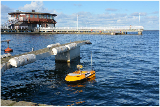
Figure 2.
OceanAlpha USV SL20 during bathymetric surveys in Puck marina.
During bathymetric surveys, it moves with a velocity of 2–5 kn, which enables both line keeping and steering. The data are transmitted via a radio link at a frequency of 2.4 GHz. A manipulator that allows two engines to be controlled separately is used for manual steering. The USV’s basic parameters are provided in Table 1.

Table 1.
Technical specification of the OceanAlpha USV SL20.
Topcon HiPer II GPS/GLONASS receiver was used for positioning purposes. In order to ensure precise horizontal positioning, the TPI NET pro network with a NET_RTCM3 correction stream dedicated to two satellite systems with the accuracy of horizontal coordinate determination of 3 cm (p = 0.95) was used. The parameters of the Topcon HiPer II receiver used for the study in a water region restricted by a quay are shown in Table 2. Due to the small sounding area and short survey lines, Real-Time Network (RTN) mode has been used during the surveys. In the case of the long survey lines and RTN mode, the virtual reference station can be moved, causing a lack of determined coordinates for automatic navigation and collecting spatial data.
Table 2.
Basic parameters of Topcon HiPer II receiver.
HYPACK (HYPACK, Middletown, CT, USA) software is used for the recording of geospatial data during a bathymetric sounding.
2.4. Planning of Survey Lines for Determining the Minimum Distance to the Quay
To determine the general course of the isobaths (shallow areas) within the hydro-engineering structure area, the survey lines were designed in an arrangement parallel to the southern quay and to each other at a distance of 2 m. The start of a survey line is located at a distance of 60 m from the western quay so that the USV can stabilise its course after entering a line. The end of the line was planned at a distance of 5 m and then reduced each time by 0.5 m. After entering the first line, the USV approached the quay and then made a turn onto another line. Then, after entering the third survey line, it again approached the quay while making a turn at a pre-set distance from it. Thus, the USV made a turn twice at a pre-set distance from the quay. The next test was conducted at a distance shorter by 0.5 m from the previous one to the safe navigation limit.
The parameter determining the quality of the USV’s line-keeping is XTE. For hydrographic surveys, the planned lines are separate sections, and the most important thing is to obtain the minimum XTE value. In an open water region, when the sounding vessel is controlled manually, there is enough room to make a turn to the next line. In a restricted water region, each line is most often started on the open side and ended near a hydro-engineering structure. Where the USV is controlled automatically, the survey lines are arranged into a broken line, and the USV moves on to the next line via the section connecting the end of the previous line with the start of the next one. A 90° turn is made twice, and the accuracy of entering the next line affects the quality of sounding within the hydro-engineering structure area.
In order to assess the quality of guiding a sounding vessel along survey lines within a hydro-engineering structure area [54,55,56,57,58,59], the following methodology was applied using XTE:
- At a distance to the end of the line longer than the distance between the lines, XTE is determined to the current line;
- At a distance to the end of the line shorter than the distance between the lines, XTE is determined to the current line and the connection between the lines;
- Where the distance to the connector is shorter than that to the line, XTE is determined to the connector and the next line;
- Where the distance to the next line is shorter than that to the connector, XTE is determined to the next line.
Phases for determining XTE to lines are presented in Figure 3.
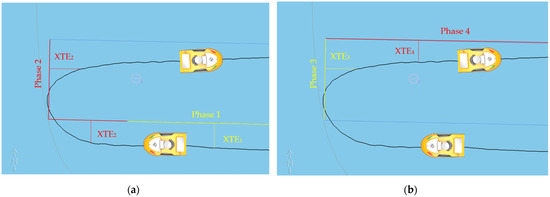
Figure 3.
Phases of XTE determination: 1 and 2 (a); 3 and 4 (b).
The main arrangement of survey lines (a full line) and their limitation every 0.5 m within the range of 1–5 m from the quay (a broken line) are presented in Figure 4.
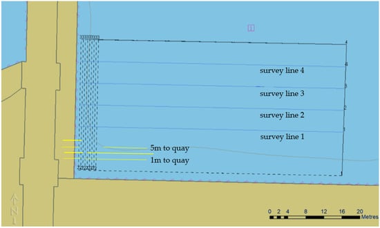
Figure 4.
The main arrangement of survey lines (a full line) and their limitation.
2.5. Determination of the USV’s Circulation Radius When Changing a Line
During the change of the line, the USV made a turn of 180°, which can be considered part of the circulation. When determining the vessel’s manoeuvring parameters, the following circulation phases are distinguished:
- Phase 1: the beginning of the circulation—the moment of laying the rudder. When the vessel has reached full velocity and the rudder is laying to the required position (35° or 15°), the following phenomena can be observed: a hydrodynamic force is generated, which disturbs the equilibrium condition existing before the start of the manoeuvre; there is a counteraction of the course inertial force, which causes the vessel’s deflection opposite to the laid rudder; or the vessel does not change the course, but its initial velocity decreases (up to 10%). The duration of this phase is determined by the size of the vessel (0.5–1 min).
- Phase 2: begins when the vessel starts to change course. The vessel’s line of symmetry deviates from the direction determined by the tangent to the curvature of the centre of gravity path, forming an increasing drift angle. The vessel’s velocity continues to decrease, the turn’s angular velocity increases, and the initial spiral curvature radius decreases.
- Phase 3: fixed circulation—the moment when hydrostatic forces reach equilibrium. The drift angle, angular velocity, linear velocity and curvature angle are constant. The end of the circulation is reached when the vessel enters the same course on which the manoeuvre started—the change in the vessel’s course is within 360°.
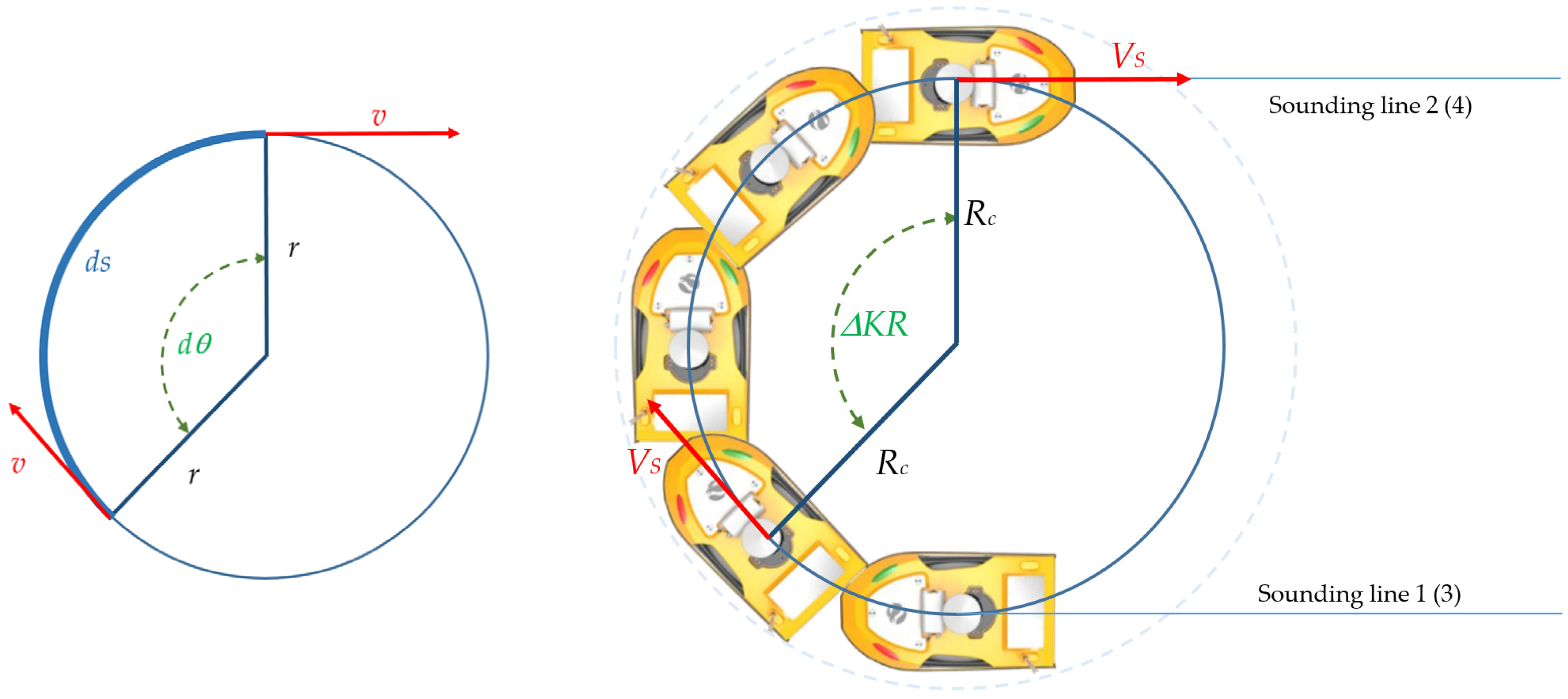
The circulation radius is directly proportional to the linear velocity; hence, the greater the vessel’s velocity, the greater the circulation, and the circulation diameter are inversely proportional to the angular velocity (Figure 5). The greater the angular velocity of the turn, the smaller the circulation. The fixed circulation diameter DU is used to denote the diameter of a circle determined by the vessel’s centre of gravity at the fixed circulation phase. The vessel’s manoeuvrability rate (K) is the DU to L ratio.
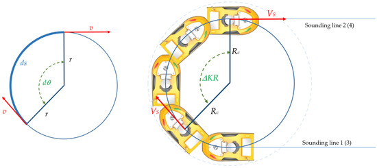
Figure 5.
Circulation of the vessel.
As a result of the effect of hydrodynamic forces causing the turn, the vessel’s line of symmetry deviates from the direction determined by the tangent to the path curvature. The same direction of deviation results in the phenomenon of the bow moving on the internal side of the circulation path and the stern moving on the external side. The angle between the tangent to the path curvature and the vessel’s line of symmetry is referred to as drift angle βC. In practice, the vessel’s linear velocity Vs represents the ratio of the distance covered by the vessel Ds to the time ΔT′:
where: ω—the vessel’s angular velocity [rad/s], dθ—the measure of the passed angle [rad], dt—the time of manoeuvre [s], ds—the length of the arc of circle’s curvature [m], v—the resultant longitudinal velocity [m/s], r—the circle’s curvature radius [m], Vs—the vessel’s velocity [w], Rc—the radius of the curvature of the vessel’s movement trajectory along the circle [Mm], ROT—rate of turn—the vessel’s angular velocity [°/min], ΔKR—the course change magnitude [°], ΔT—the manoeuvre duration [min].
Figure 6 presents USV’s circulations during the survey line change manoeuvre.
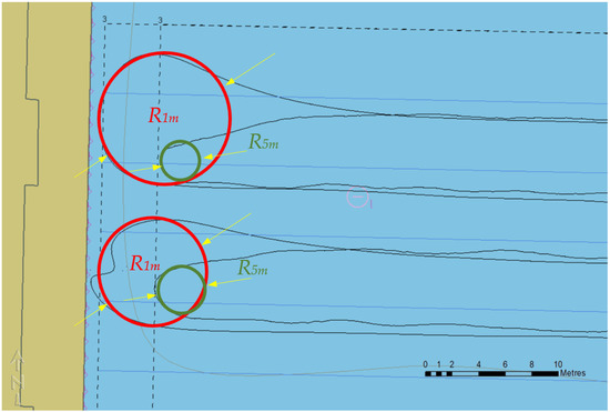
Figure 6.
USV’s circulations during the manoeuvre of survey line change.
3. Results
The study results are presented in three groups: at a distance of 5 m, 4.5 m, and 4 m (Section 3.1); 3.5 m, 3 m, and 2.5 m (Section 3.2), and 2 m, 1.5 m and 1 m (Section 3.3) from the quay. The shortest distance from the quay results from the USV’s size and the position of the GNSS antenna in relation to the sides, the bow and the stern. When attempting to make a turn at a distance of 0.5 m from the quay, where the GNSS antenna’s distance to the bow is 52 cm, the probability of the USV’s contact with the quay is very high. Therefore, surveys were only performed at a distance of 1 m to the quay.
Based on the current USV’s position, XTE was determined for survey line 1 at Phase 1 of the circulation, to the line connecting lines 1 and 2 at Phase 2 and 3, and to line 3 at Phase 4. The same methodology was applied on the next turn within the hydro-engineering structure area, i.e., for lines 3 and 4 (Figure 3). No circulation was examined when switching from line 2 to line 3, as it was performed in an open water region.
3.1. Distance to the Quay of 5–4 m
Within this range of the distance from the quay, the USV maintained the minimum (0.2 m) distance from the limit of the sounding area to ensure safe navigation. The sounding area limit was not exceeded (Figure 7). It can be noted that while leaving a survey line (both 1 and 3) is dynamic, entering the next survey line (2 and 4) is conservative, as the USV enters the line smoothly, which makes the XTE value in the initial phase the highest.
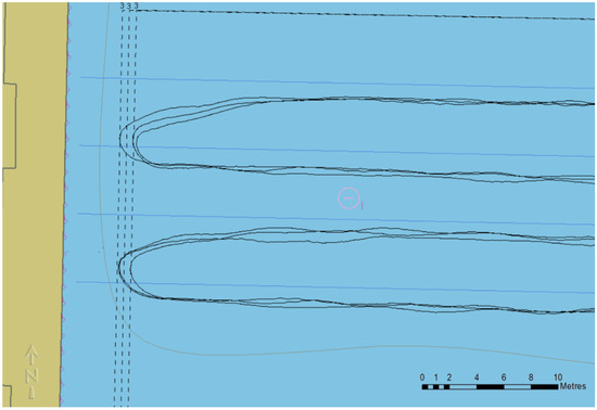
Figure 7.
Trajectory of USV in the distance of 5 m, 4.5 m and 4 m to the quay.
Based on [45] and the presented study, it can be observed that USV SL20 tends toward a significant (1–1.5 m) deviation (XTE) from the survey lines on the E–W (east–west) direction while keeping on the N–S (north–south) lines. The course fluctuations result from having made a turn, while the velocity is adjusted to the conditions of its execution: it decreases when the turn is being made and increases when it has been completed (Table 3). A negative value of XTE means that the USV was on the left of the sounding line; positive means on the right of the sounding line.
Table 3.
Cross-track error XTE and speed over ground SOG in the distance of 5 m, 4.5 m and 4 m to the quay.
The circulation diameter is smaller than the distance between the lines. It can be noted that USV lays down on the next survey line while performing half a circulation and changing the course in the range of up to 180°. Figure 8 shows the course over ground SOG and speed over ground SOG in the distance of 5 m, 4.5 m and 4 m to the quay.
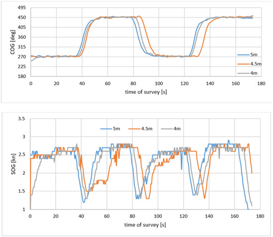
Figure 8.
Course over ground COG and speed over ground SOG in the distance of 5 m, 4.5 m and 4 m to the quay.
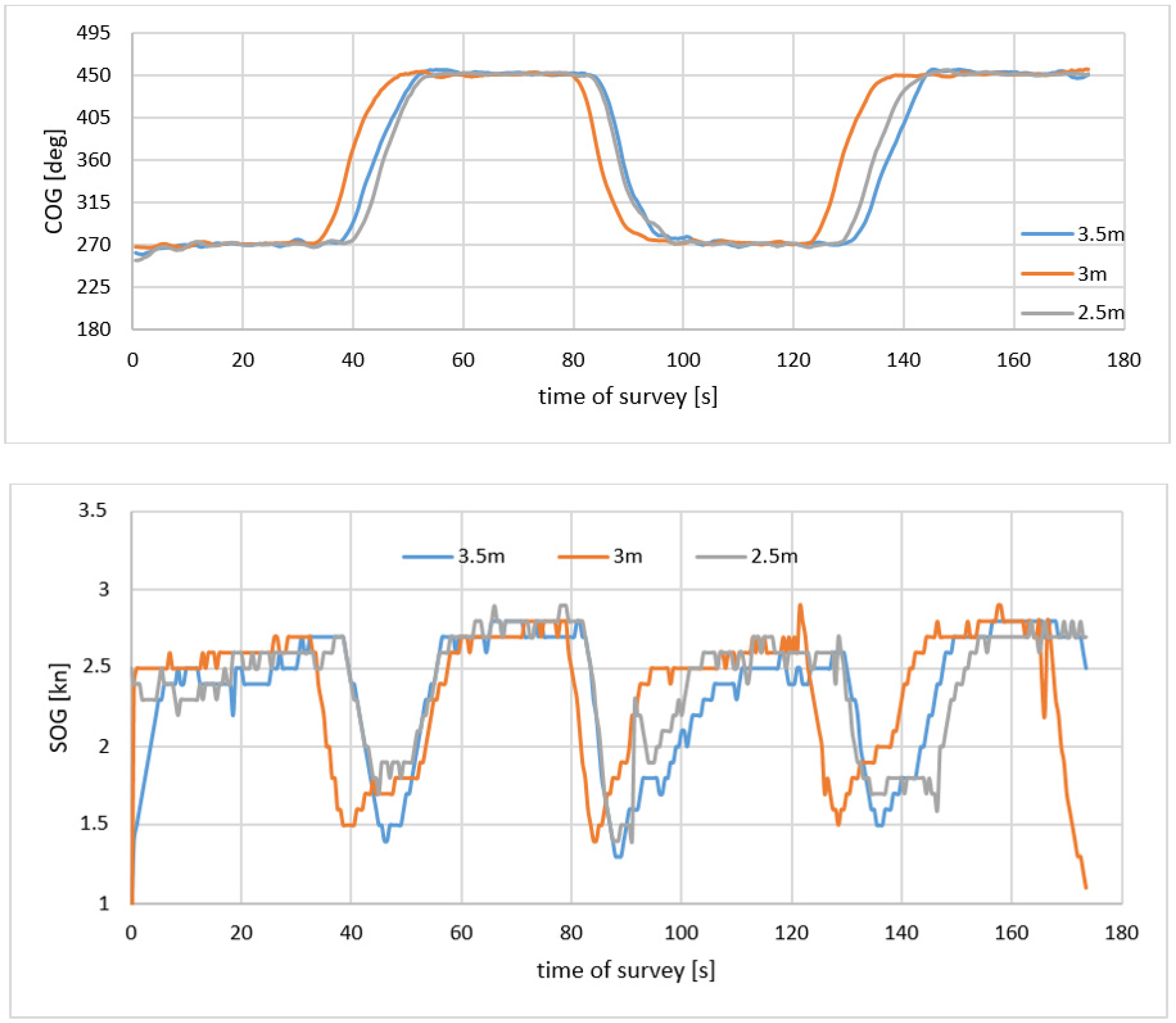
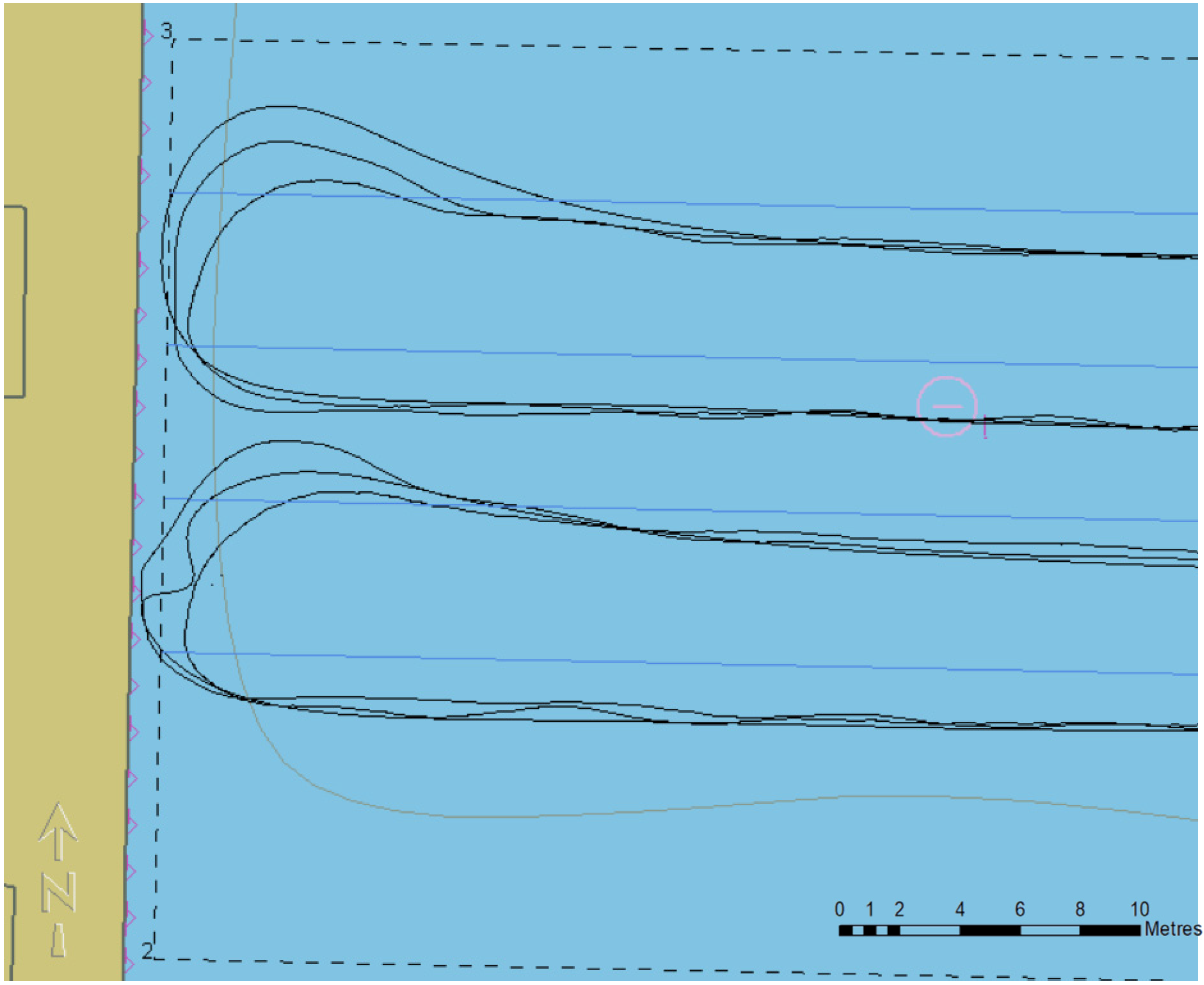
3.2. Distance to the Quay of 3.5–2.5 m
Within the distance range of 3.5–2.5 m to the quay, it can be observed that the circulation radius increases when the USV enters the next survey line (Figure 9). On the one hand, the USV proceeds to the sounding area limit, thus ensuring the survey of geospatial data to the end of the line.
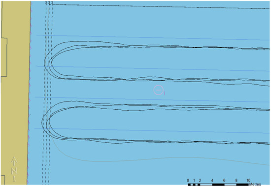
Figure 9.
The trajectory of USV in the distance of 3.5 m, 3 m and 2.5 m to the quay.
On the other hand, moving outside the sounding area poses a threat to the USV’s navigation safety. In addition to XTE on a line, the most important parameter during a turn onto the next survey line is the distance to the quay as an XTE relative value on sections 1–2 and 3–4.
Cross-track error XTE and speed over ground SOG of the USV are provided in Table 4, and course over ground SOG and speed over ground SOG in the graphical form, in Figure 10.
Table 4.
Cross-track error XTE and speed over ground SOG in the distance of 3.5 m, 3 m and 2.5 m to the quay.
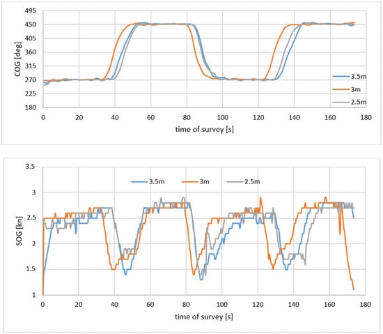
Figure 10.
Course over ground SOG and speed over ground SOG in the distance of 3.5 m, 3 m and 2.5 m to the quay.
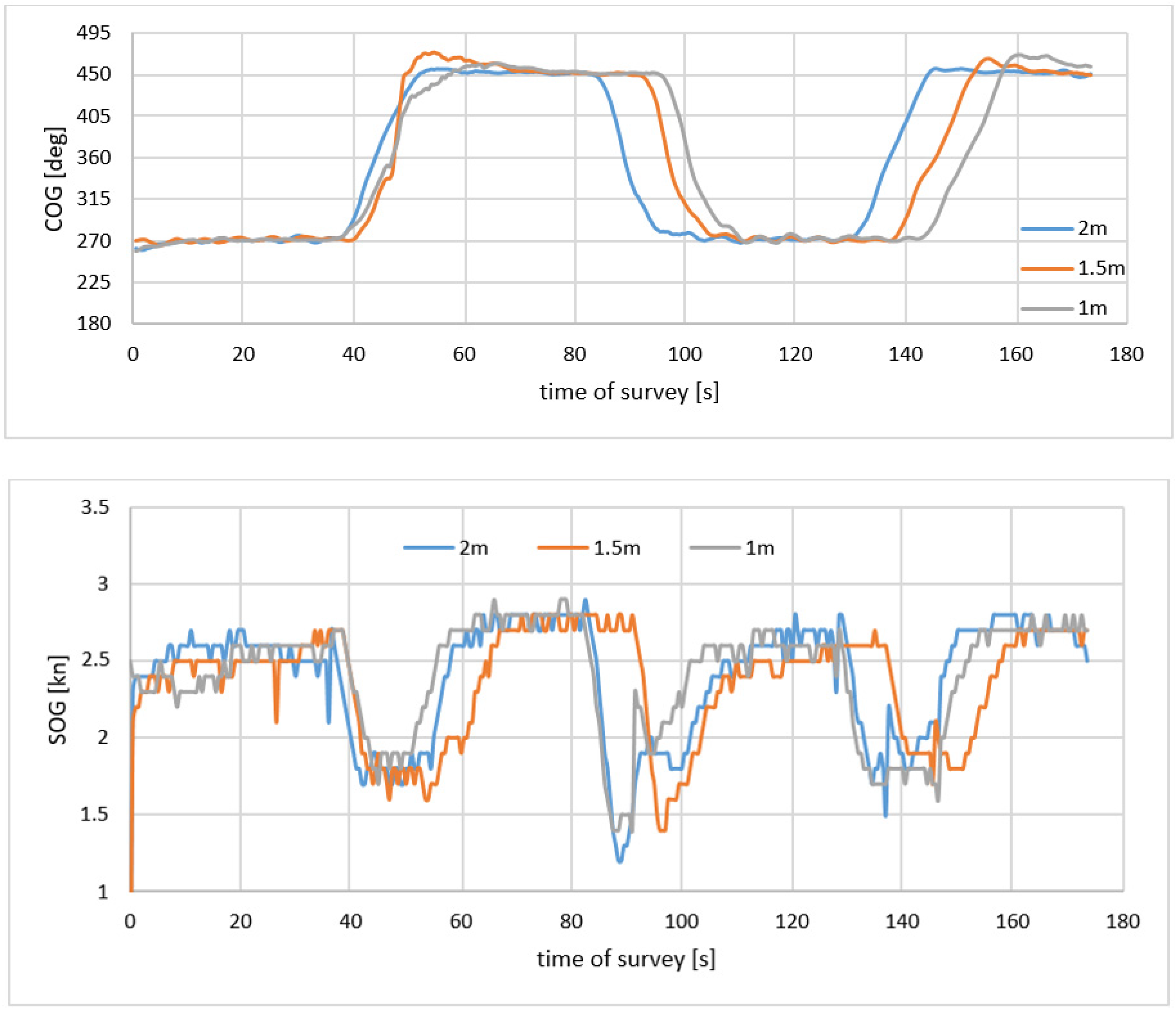
3.3. Distance to the Quay of 2–1 m
The greatest navigation safety (avoidance of the danger of USV’s collision with the quay) should be ensured at the shortest distance from the hydro-engineering structure. It could be assumed that the USV moves along a survey line with a low XTE value, and before its end or after crossing it, it makes the first 90° turn on the spot. After reaching the next survey line, it then makes another 90° turn. In fact, the manoeuvring parameters, the steering system and the external factors do not guarantee the USV’s line-keeping (Figure 11).

Figure 11.
Trajectory of USV in the distance of 2 m, 1.5 m and 1 m to the quay.
While the sounding area limit is not exceeded on longer distances (2 m and 1.5 m), for the lines nearest to the quay (1 m), the USV came into contact with the quay. The increasing circulation radius is another threat to the objects for which this line borders other objects.
Cross-track error XTE and speed over ground SOG of the USV are provided in Table 5, and the course over ground SOG and speed over ground SOG in graphical form in Figure 12.
Table 5.
Cross-track error XTE and speed over ground SOG in the distance of 2 m, 1.5 m and 1 m to the quay.
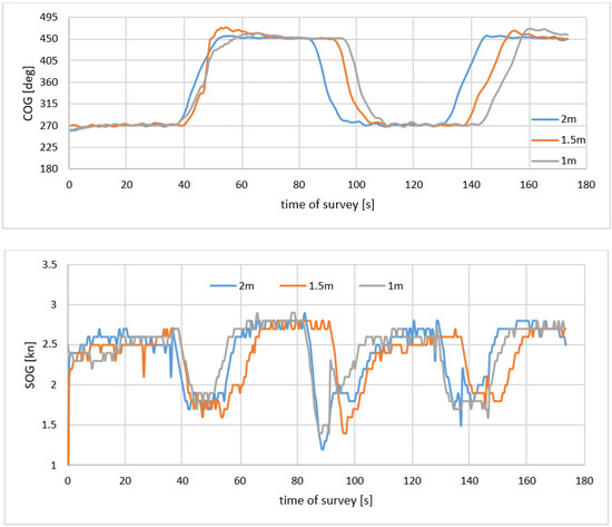
Figure 12.
Course over ground SOG and speed over ground SOG in the distance of 2 m, 1.5 m and 1 m to the quay.
4. Discussion
In order to meet the requirements imposed on bathymetric surveys and to obtain the highest reliability of DBSM, it is necessary to keep the USV on the survey line. It is not equivalent to keeping the course, as the vessel is subject to external and internal disturbances. A small vessel is susceptible to the effects of current and wind, which result in a deviation from the line, i.e., XTE. Deviation also occurs when the autopilot regulator settings are incorrectly selected, in particular when too large an insensitivity zone, also referred to as a yaw zone, has been set.
In order to gain control over the (USV) steering system, a control system is applied that will determine the effect of the interference signal e(t) on the output signal u(t), and, based on a comparison of the input signal e(t) and output signal u(t), will determine a decision. In order to control a vessel, adaptation-type regulators are most commonly applied. Their dynamic properties are optimised by the automatic adaptation of the object’s operating conditions. The adaptation refers here to the tuning of parameters of the regulator that contains the adaptation path to the variable parameters of the vessel as an object under control. The movement of a vessel is determined by a number of quantities, including the rudder laying angle, propeller rotational speed, wind, and waves. In vessels with no rudder, the movement is determined by two engines. These requirements are met by a PID-type regulating device [60,61,62,63,64,65,66,67,68,69], i.e., one with the following equation:
In Equation (4), the input signal of the PID regulator influences the weighted sum, where the weight of the proportional element is determined by P coefficient, integrating element by coefficient, and differentiating element by , where P is the volume of the regulator, TI is time of integration and TD is time of differentiation.
The tuning of P, I and D coefficients is effected automatically [70,71,72] or manually [73] during sea trials. They pertain, respectively, to the amplification of proportional, integral and derivative terms. An unmanned surface vehicle that conducts a mission autonomously should be navigated in a way that makes it possible to reach the next waypoint in the shortest time possible. However, this approach differs from the approach required in hydrographic surveys, which consists of the fact that the USV should navigate as close as possible to the planned sounding profile.
The study recorded the coordinates of the position of the GNSS antenna installed on the USV and the course and velocity. XTE was determined based on the position coordinates in relation to the survey profiles. Based on the USV’s trajectory, the circulation radius was determined by the graphical method. On the basis of this relationship (3), minimum and maximum values of rate of turn (ROT) were calculated (Table 6).
Table 6.
Circulation radius and rate of turn—ROT.
During the survey, the USV was keeping constant velocity. It changed when the USV was turning to another survey line and the circulation radius was different. In long distances to the quay, the radius was small and it guaranteed safe turning. Approaching the quay (sounding lines are longer and closer to the quay), the circulation radius increased and USV exceeded the sounding area (negative value of XTE). A high rate of turn was reached when the circulation radius was small and the average of linear velocity was constant. The risk of realization of the sounding should be searched in the parameters of the autopilot.
5. Conclusions
Bathymetric surveys in restricted water regions, e.g., in harbours, shipyard basins, marinas and coastal areas, are performed using USVs. Their advantages include small size, high manoeuvrability and being unmanned. The least labour-intensive and time-consuming mode of operation is automatic navigation, which is expected to ensure the sounding vessel’s line-keeping. In the areas of a hydro-engineering structure belonging to the International Hydrographic Organization (IHO) Special or Exclusive Order, the requirements for the accuracy of positioning and sounding as a whole are the highest. Performing a survey using a vehicle moving on water in the immediate vicinity of a structure is not easy, and increasing the surveying distance from the structure results in geospatial data loss.
The use of geodetic positioning methods with accuracy in the order of 1–2 cm (p = 0.95) offers the possibility for the densification of survey lines (decreasing the distances between them) and the manoeuvring near the quay, breakwater, or other harbour facilities. The limitations include: the size of the USV and the position of the GNSS antenna; the accuracy of positioning in a water region with difficult observational conditions; manoeuvring parameters (circulation diameter, and the vessel’s line-keeping (XTE → 0). Positioning the GNSS antenna at a distance of approximately 0.5 m from the bow and the stern is expected to ensure a slightly longer distance between the bathymetric surveys and the structure. Under difficult observational conditions, the positioning accuracy is lower, affecting data accuracy (reliability) and the USV’s navigation safety.
When the circulation diameter is large, and the sounding area has been crossed, it is reasonable to increase the distance from the quay and perform surveys on the survey line(s) parallel to it. Their number is determined by the distance of the lines perpendicular to the quay. The method performs well with long and unrestricted quays. However, this becomes more complicated in corners and hydrographically complicated water regions, e.g., in marinas. Maneuvering between floating platforms (Y-booms) is dangerous to the USV, and performing a survey along the quay near the platforms is impossible. For each sounding vessel, the navigational (positioning and manoeuvring) capabilities should be verified under different observational and hydrometeorological conditions. For a 1 m-long USV used for measurements (hydrographic surveys) with no wind and current as disruptive external factors and positioning in RTN mode, a 1 m safe distance between a quay to the end of the survey line can be established.
Funding
This research received no external funding.
Institutional Review Board Statement
Not applicable.
Informed Consent Statement
Not applicable.
Data Availability Statement
Not applicable.
Conflicts of Interest
The author declares no conflict of interest.
References
- Remondino, F.; Barazzetti, L.; Nex, F.; Scaioni, M.; Sarazzi, D. UAV photogrammetry for mapping and 3d modelling-current status and future perspectives. In Proceedings of the International Archives of the Photogrammetry, Remote Sensing and Spatial Information Sciences, Zurich, Switzerland, 14–16 September 2011; Volume 38, p. C22. [Google Scholar]
- Nex, F. UAV-g 2019: Unmanned Aerial Vehicles in Geomatics. Drones 2019, 3, 74. [Google Scholar] [CrossRef] [Green Version]
- Colomina, I.; Molina, P. Unmanned aerial systems for photogrammetry and remote sensing: A review. ISPRS J. Photogramm. Remote Sens. 2014, 92, 79–97. [Google Scholar] [CrossRef] [Green Version]
- Özcan, O.; Akay, S.S. Modeling Morphodynamic Processes in Meandering Rivers with UAV-Based Measurements. In Proceedings of the IGARSS 2018—2018 IEEE International Geoscience and Remote Sensing Symposium, Valencia, Spain, 22–27 July 2018; pp. 7886–7889. [Google Scholar]
- Burdziakowski, P.; Specht, C.; Dabrowski, P.S.; Specht, M.; Lewicka, O.; Makar, A. Using UAV Photogrammetry to Analyse Changes in the Coastal Zone Based on the Sopot Tombolo (Salient) Measurement Project. Sensors 2020, 20, 4000. [Google Scholar] [CrossRef] [PubMed]
- Agrafiotis, P.; Skarlatos, D.; Georgopoulos, A.; Karantzalos, K. Shallow water bathymetry mapping from UAV imagery based on machine learning. Int. Arch. Photogramm. Remote Sens. Spat. Inf. Sci. 2019, XLII-2/W10, 9–16. [Google Scholar]
- Hashimoto, K.; Shimozono, T.; Matsuba, Y.; Okabe, T. Unmanned aerial vehicle depth inversion to monitor river-mouth bar dynamics. Remote Sens. 2021, 13, 412. [Google Scholar] [CrossRef]
- Jin, J.; Zhang, J.; Shao, F.; Lyu, Z.; Wang, D. A novel ocean bathymetry technology based on an unmanned surface vehicle. Acta Oceanol. Sin 2018, 37, 99–106. [Google Scholar] [CrossRef]
- Bruzzone, G.; Bibuli, M.; Caccia, M. Improving coastal operations with unmanned surface vehicles. Sea Technol. 2011, 52, 46–49. [Google Scholar]
- Liu, Z.; Zhang, Y.; Yu, X.; Yuan, C. Unmanned Surface Vehicles: An Overview of Developments and Challenges. Ann. Rev. Control 2016, 41, 71–93. [Google Scholar] [CrossRef]
- Specht, M.; Specht, C.; Szafran, M.; Makar, A.; Dąbrowski, P.; Lasota, H.; Cywiński, P. The Use of USV to Develop Navigational and Bathymetric Charts of Yacht Ports on the Example of National Sailing Centre in Gdańsk. Remote Sens. 2020, 12, 2585. [Google Scholar] [CrossRef]
- Makar, A.; Specht, C.; Specht, M.; Dąbrowski, P.; Szafran, M. Integrated Geodetic and Hydrographic Measurements of the Yacht Port for Nautical Charts and Dynamic Spatial Presentation. Geosciences 2020, 10, 203. [Google Scholar] [CrossRef]
- Makar, A.; Specht, C.; Specht, M.; Dąbrowski, P.; Burdziakowski, P.; Lewicka, O. Seabed Topography Changes in the Sopot Pier Zone in 2010–2018 Influenced by Tombolo Phenomenon. Sensors 2020, 20, 6061. [Google Scholar] [CrossRef] [PubMed]
- International Hydrographic Organization. IHO Standards for Hydrographic Surveys, 6th ed.; Special Publication No. 44; IHO: Monte Carlo, Monaco, 2018. [Google Scholar]
- International Hydrographic Organization. Manual on Hydrography, 1st ed.; Publication C-13; IHO: Monte Carlo, Monaco, 2005. [Google Scholar]
- Canadian Hydrographic Service. CHS Standards for Hydrographic Surveys, 2nd ed.; CHS: Ottawa, ON, Canada, 2013. [Google Scholar]
- National Oceanic and Atmospheric Administration. NOS Hydrographic Surveys Specifications and Deliverables; NOAA: Silver Spring, MD, USA, 2017. [Google Scholar]
- Ministry of Defence. Act of 28 March 2018 on the Minimum Standards for Hydrographic Surveys, 2018; Ministry of Defence: Warsaw, Poland, 2018. (In Polish)
- Hydrographic Office of the Polish Navy. Maritime Hydrography—Organization and Research Rules; Hydrographic Office of the Polish Navy: Gdynia, Poland, 2009. [Google Scholar]
- Hydrographic Office of the Polish Navy. Maritime Hydrography—Rules of Data Collecting and Results Presentation; Hydrographic Office of the Polish Navy: Gdynia, Poland, 2009. [Google Scholar]
- Nex, F.; Remondino, F. UAV for 3D mapping applications: A review. Appl. Geomat. 2014, 6, 1–15. [Google Scholar] [CrossRef]
- Torresan, C.; Berton, A.; Carotenuto, F.; Di Gennaro, S.F.; Gioli, B.; Matese, A.; Miglietta, F.; Vagnoli, C.; Zaldei, A.; Wallace, L. Forestry applications of UAVs in Europe: A review. Int. J. Remote Sens. 2017, 38, 2427–2447. [Google Scholar] [CrossRef]
- Müllenstedt, D.; Schmidt, J.; Fügenschuh, A. Mission Planning for Unmanned Aerial Vehicles; Cottbus Mathematical Preprints; Brandenburg University of Technology: Cottbus, Germany, 2019. [Google Scholar] [CrossRef]
- Shahid, N.; Muhammad, A.; Ajmal, U.; Masroor, R.; Amjad, S.; Jeelani, M. Path planning in unmanned aerial vehicles: An optimistic overview. Int. J. Commun. Syst. 2022, 35, e5090. [Google Scholar] [CrossRef]
- Stateczny, A.; Kazimierski, W.; Burdziakowski, P.; Motyl, W.; Wisniewska, M. Shore Construction Detection by Automotive Radar for the Needs of Autonomous Surface Vehicle Navigation. ISPRS Int. J. Geo-Inf. 2019, 8, 80. [Google Scholar] [CrossRef] [Green Version]
- Giordano, F.; Mattei, G.; Parente, C.; Peluso, F.; Santamaria, R. MicroVEGA (Micro Vessel for Geodetics Application): A Marine Drone for the Acquisition of Bathymetric Data for GIS Applications. Int. Arch. Photogramm. Remote Sens. Spat. Inf. Sci. 2015, 40, 123–130. [Google Scholar] [CrossRef] [Green Version]
- Giordano, F.; Mattei, G.; Parente, C.; Peluso, F.; Santamaria, R. Integrating Sensors into a Marine Drone for Bathymetric 3D Surveys in Shallow Waters. Sensors 2016, 16, 41. [Google Scholar] [CrossRef] [Green Version]
- Popielarczyk, D.; Templin, T.; Ciecko, A.; Grunwald, G. Application of GNSS and SBES techniques to investigate the Lake Suskie bottom shape. In Proceedings of the 16th International Multidisciplinary Scientific GeoConference SGEM, Albena, Bulgaria, 28 June–6 July 2016; Book 2. Volume 2, pp. 109–116. [Google Scholar] [CrossRef]
- Popielarczyk, D.; Templin, T.; Lopata, M. Using the geodetic and hydroacoustic measurements to investigate the bathymetric and morphometric parameters of Lake Hańcza (Poland). Open Geosci. 2015, 7, 1–16. [Google Scholar] [CrossRef]
- Popielarczyk, D.; Templin, T. Application of Integrated GNSS/Hydroacoustic Measurements and GIS Geodatabase Models for Bottom Analysis of Lake Hancza. Pure Appl. Geophys. 2014, 171, 997–1011. [Google Scholar] [CrossRef] [Green Version]
- Bakuła, M.; Oszczak, S.; Pelc-Mieczkowska, R. Performance of RTK positioning in forest conditions: Case study. J. Surv. Eng. 2009, 3, 125–130. [Google Scholar] [CrossRef]
- Bakuła, M.; Oszczak, S. Experiences of RTK positioning in hard observational conditions during Nysa Kłodzka river Project. Rep. Geod. 2006, 1, 71–79. [Google Scholar]
- Bakuła, M.; Pelc-Mieczkowska, R.; Walawski, M. Reliable and redundant RTK positioning for applications in hard observational conditions. Artif. Satell. 2012, 47, 23–33. [Google Scholar] [CrossRef]
- Specht, C.; Makar, A.; Specht, M. Availability of the GNSS Geodetic Networks Position during the Hydrographic Surveys in the Ports. TransNav Int. J. Mar. Navig. Saf. Sea Transp. 2018, 12, 657–661. [Google Scholar] [CrossRef]
- Lohan, E.S.; Borre, K. Accuracy Limits in Multi-GNSS. IEEE Trans. Aerosp. Electron. Syst. 2017, 52, 2477–2494. [Google Scholar] [CrossRef]
- Jang, W.S.; Park, H.S.; Seo, K.Y.; Kim, Y.K. Analysis of positioning accuracy using multi differential GNSS in coast and port area of South Korea. J. Coast. Res. 2016, 75, 1337–1341. [Google Scholar] [CrossRef]
- Ziquan, H.; Xiufeng, H.; Liu, Z.; Sang, W. Analysis of the DOP Values and Availability of Combined GPS/GLONASS/GALILEO Navigation System. GNSS World China 2012, 37, 32–37. [Google Scholar]
- Makar, A. Dynamic Tests of ASG-EUPOS Receiver in Hydrographic Application. In Proceedings of the 18th International Multidisciplinary Scientific GeoConference SGEM, Albena, Bulgaria, 30 June–9 July 2018; Volume 18, pp. 743–750. [Google Scholar]
- Maciuk, K. GPS-only, GLONASS-only and Combined GPS+GLONASS Absolute Positioning under Different Sky View Conditions. Teh. Vjesn. 2018, 25, 933–939. [Google Scholar]
- Hasan, M.; Rouf, R.R.; Islam, S. Investigation of Most Ideal GNSS Framework (GPS, GLONASS and GALILEO) for Asia Pacific Region (Bangladesh). Int. J. Appl. Inf. Syst. 2017, 12, 33–37. [Google Scholar] [CrossRef]
- Makar, A. Determination of Inland Areas Coastlines. In Proceedings of the 18th International Multidisciplinary Scientific GeoConference SGEM, Albena, Bulgaria, 2–8 July 2018; Volume 18, pp. 701–708. [Google Scholar]
- Baptista, P.; Bastos, L.; Bernardes, C.; Cunha, T.; Dias, J. Monitoring Sandy Shores Morphologies by DGPS—A Practical Tool to Generate Digital Elevation Models. J. Coast. Res. 2008, 24, 1516–1528. [Google Scholar] [CrossRef]
- Yayla, G.; Baelen, S.; Peeters, G.; Afzal, M.R.; Catoor, T.; Singh, Y.; Slaets, P. Accuracy Benchmark of Galileo and EGNOS for Inland Waterways. In Proceedings of the International Ship Control Systems Symposium (ISCSS), Delft, The Netherlands, 6–8 October 2020. [Google Scholar] [CrossRef]
- Yayla, G.; Christofakis, C.; Storms, S.; Catoor, T.; Pilozzi, P.; Singh, Y.; Peeters, G.; Afzal, M.R.; Van Baelen, S.; Holm, D.; et al. Measuring the Impact of a Navigation Aid in Unmanned Ship Handling via a Shore Control Center. In Advances in Human Factors in Robots, Unmanned Systems and Cybersecurity; Zallio, M., Raymundo Ibañez, C., Hernandez, J.H., Eds.; Lecture Notes in Networks and Systems; Springer: Cham, Switzerland, 2021; Volume 268. [Google Scholar] [CrossRef]
- Ministry of Transport, Construction and Maritime Economy. Ordinance of the Minister of Transport, Construction and Maritime Economy of 1 June 1998 on the Technical Conditions That Should Be Met by Marine Hydraulic Structures and Their Location, 1998; Ministry of Transport, Construction and Maritime Economy: Warsaw, Poland, 1998. (In Polish)
- Ministry of Transport, Construction and Maritime Economy. Ordinance of the Minister of Transport, Construction and Maritime Economy of 23 October 2006 on the Technical Conditions for the Use of Marine Hydraulic Structures and the Detailed Scope of Inspections to Be Carried out on Such Structures, 2006; Ministry of Transport, Construction and Maritime Economy: Warsaw, Poland, 2006. (In Polish)
- Marchel, Ł.; Specht, C.; Specht, M. Assessment of the Steering Precision of a Hydrographic USV along Sounding Profiles Using a High-Precision GNSS RTK Receiver Supported Autopilot. Energies 2020, 13, 5637. [Google Scholar] [CrossRef]
- Specht, M.; Specht, C.; Lasota, H.; Cywiński, P. Assessment of the Steering Precision of a Hydrographic Unmanned Surface Vessel (USV) along Sounding Profiles Using a Low-cost Multi-Global Navigation Satellite System (GNSS) Receiver Supported Autopilot. Sensors 2019, 19, 3939. [Google Scholar] [CrossRef] [PubMed] [Green Version]
- Stateczny, A.; Burdziakowski, P.; Najdecka, K.; Domagalska-Stateczna, B. Accuracy of Trajectory Tracking Based on Nonlinear Guidance Logic for Hydrographic Unmanned Surface Vessels. Sensors 2020, 20, 832. [Google Scholar] [CrossRef] [PubMed] [Green Version]
- Singh, Y.; Sharma, S.; Sutton, R.; Hatton, D.; Khan, K. A constrained A* approach towards optimal path planning for an unmanned surface vehicle in a maritime environment containing dynamic obstacles and ocean currents. Ocean. Eng. 2018, 169, 187–201. [Google Scholar] [CrossRef] [Green Version]
- Cloet, R.L. The Effect of Line Spacing on Survey Accuracy in a Sand-wave Area. Hydrogr. J. 1976, 2, 5–11. [Google Scholar]
- Bouwmeester, E.C.; Heemink, A.W. Optimal Line Spacing in Hydrographic Survey. Int. Hydrogr. Rev. 1993, LXX, 37–48. [Google Scholar]
- Yang, Y.; Li, Q.; Zhang, J.; Xie, Y. Iterative Learning-based Path and Speed Profile Optimization for an Unmanned Surface Vehicle. Sensors 2020, 20, 439. [Google Scholar] [CrossRef] [Green Version]
- Rutkowski, G. ECDIS Limitations, Data Reliability, Alarm Management and Safety Settings Recommended for Passage Planning and Route Monitoring on VLCC Tankers. TransNav Int. J. Mar. Navig. Saf. Sea Transp. 2018, 12, 483–490. [Google Scholar] [CrossRef]
- Rutkowski, G. Determining the Best Possible Speed of the Ship in Shallow Waters Estimated Based on the Adopted Model for Calculation of the Ship’s Domain Depth. Polish Marit. Res. 2020, 27, 140–148. [Google Scholar] [CrossRef]
- Rutkowski, G. Determining Ship’s Safe Speed and Best Possible Speed for Sea Voyage Legs. TransNav Int. J. Mar. Navig. Saf. Sea Transp. 2016, 10, 3. [Google Scholar] [CrossRef] [Green Version]
- Rutkowski, G. Determining the Ship’s Optimal Speed and Safe Track Selection on the Circle on the Narrow and Sharp Bend Fairways by means of the Rate of Turn ROT Techniques. Sci. J. Gdyn. Marit. Univ. 2017, 102, 70–79. [Google Scholar]
- Novaselic, M.; Mohović, R.; Baric, M.; Grbić, L. Wind Influence on Ship Manoeuvrability—A Turning Circle Analysis. TransNav Int. J. Mar. Navig. Saf. Sea Transp. 2021, 15, 47. [Google Scholar] [CrossRef]
- Cui, J.; Wu, Z.; Chen, W. Research on Prediction of Ship Manoeuvrability. J. Shipp. Ocean. Eng. 2018, 8, 30–35. [Google Scholar] [CrossRef]
- Naus, K.; Marchel, Ł. Use of a Weighted ICP Algorithm to Precisely Determine USV Movement Parameters. Appl. Sci. 2019, 9, 3530. [Google Scholar] [CrossRef] [Green Version]
- Lv, C.; Yu, H.; Hua, Z.; Li, L.; Chi, J. Speed and Heading Control of an Unmanned Surface Vehicle Based on State Error PCH Principle. Math. Probl. Eng. 2018, 2018, 7371829. [Google Scholar] [CrossRef] [Green Version]
- Wang, L.; Wu, Q.; Liu, J.; Li, S.; Negenborn, R.R. State-of-the-art Research on Motion Control of Maritime Autonomous Surface Ships. J. Mar. Sci. Eng. 2019, 7, 438. [Google Scholar] [CrossRef] [Green Version]
- Cho, H.; Jeong, S.-K.; Ji, D.-H.; Tran, N.-H.; Vu, M.T.; Choi, H.-S. Study on Control System of Integrated Unmanned Surface Vehicle and Underwater Vehicle. Sensors 2020, 20, 2633. [Google Scholar] [CrossRef]
- Mou, J.; He, Y.; Zhang, B.; Li, S.; Xiong, Y. Path Following of a Water-jetted USV Based on Maneuverability Tests. J. Mar. Sci. Eng. 2020, 8, 354. [Google Scholar] [CrossRef]
- Aguiar, A.P.; Hespanha, J.P. Trajectory-tracking and Path following of Underactuated Autonomous Vehicles with Parametric Modeling Uncertainty. IEEE Trans. Autom. Control 2007, 52, 1362–1379. [Google Scholar] [CrossRef] [Green Version]
- Do, K.D.; Pan, J. Global Tracking Control of Underactuated Ships with Nonzero Off-diagonal Terms in Their System Matrices. Automatica 2005, 41, 87–95. [Google Scholar]
- Li, C.; Jiang, J.; Duan, F.; Liu, W.; Wang, X.; Bu, L.; Sun, Z.; Yang, G. Modeling and Experimental Testing of an Unmanned Surface Vehicle with Rudderless Double Thrusters. Sensors 2019, 19, 2051. [Google Scholar] [CrossRef] [Green Version]
- Kristić, M.; Žuškin, S.; Brčić, D.; Valčić, S. Zone of Confidence Impact on Cross Track Limit Determination in ECDIS Passage Planning. J. Mar. Sci. Eng. 2020, 8, 566. [Google Scholar] [CrossRef]
- Azar, A.T.; Ammar, H.H.; Ibrahim, Z.F.; Ibrahim, H.A.; Mohamed, N.A.; Taha, M.A. Implementation of PID Controller with PSO Tuning for Autonomous Vehicle. In Proceedings of the International Conference on Advanced Intelligent Systems and Informatics 2019 (AISI 2019), Cairo, Egypt, 26–28 October 2019. [Google Scholar]
- Miskovic, N.; Vukic, Z.; Barisic, M.; Tovornik, B. Autotuning Autopilots for Micro-ROVs. In Proceedings of the 2006 14th Mediterranean Conference on Control and Automation (MED 2006), Ancona, Italy, 28–30 June 2006. [Google Scholar]
- Pan, Y.; Huang, D.; Sun, Z. Backstepping Adaptive Fuzzy Control for Track-keeping of Underactuated Surface Vessels. Control Theory Appl. 2011, 28, 907–914. [Google Scholar]
- Chattopadhyay, S.; Roy, G.; Panda, M. Simple Design of a PID Controller and Tuning of Its Parameters Using LabVIEW Software. Sens. Transducers 2011, 129, 69–85. [Google Scholar]
- Świder, Z. A Prototype of an Advanced Ship Autopilot Implemented in the CPDev Environment. Meas. Autom. Robot. 2021, R. 25, 13–18. [Google Scholar] [CrossRef]


Publisher’s Note: MDPI stays neutral with regard to jurisdictional claims in published maps and institutional affiliations. |
© 2022 by the author. Licensee MDPI, Basel, Switzerland. This article is an open access article distributed under the terms and conditions of the Creative Commons Attribution (CC BY) license (https://creativecommons.org/licenses/by/4.0/).