1. Introduction
The presalt sequence has favourable hydrocarbon source conditions, reservoir conditions and hydrocarbon accumulation conditions, all of which have great potential for petroleum prospecting. However, oil and gas exploration in deep-water areas is high-cost and high-risk, which limits exploration processes. In addition to the general characteristics of carbonate rocks [
1,
2], presalt targets are affected by the thickness of the salt rocks, and their geophysical sensitivity properties and changing characteristics put forward higher requirements for the seismic prediction and description accuracy of high-quality reservoirs.
Deep-water presalt carbonate reservoirs have high exploration risks and high investment costs [
3]. This type of carbonate reservoir has strong heterogeneity and severe lateral variation, which makes reservoir prediction and reservoir description a major technical challenge at present [
4,
5,
6,
7]. Therefore, based on presalt geology, well logging, and prestack and poststack seismic data, research on reservoir heterogeneity and reservoir-fluid-containing geophysical characteristics was conducted to optimize the sensitive petrophysical parameters and explore the distribution of oil and gas in presalt geological targets [
8,
9]. Such work is particularly important for the optimization of exploration targets and investment decisions.
Prestack seismic inversion retains the characteristics that the seismic reflection amplitude varies with the offset or incident angle and can provide more sensitive and effective data volume results. Under the constraint of log data, prestack seismic inversion research on seismic P-wave and S-wave velocity, density and other elastic parameters is carried out to obtain high-precision elastic parameters that can reflect the lateral changes in reservoirs. Crucially, the spatial distribution of complex oil and gas reservoirs must be studied to enable researchers to create detailed descriptions of complex oil and gas reservoirs [
10,
11]. Therefore, under the constraint that data must be logged, the inversion of prestack seismic elastic parameters is carried out by using abundant prestack seismic data to obtain high-precision P-wave and S-wave velocities that can reflect the lateral changes in reservoirs. On this basis, the P-wave and S-wave velocity ratio section, Poisson’s ratio section, gas-zone indicator section and fluid-factor section can be obtained, all of which can provide more information for geological interpretation, in addition to realizing quantitative predictions of oil and gas reservoirs, narrowing the solution options, improving the drilling success rate and reducing exploration risk.
The prestack inversion used in industrial production generally employs partial stacking data to establish an initial model, and then through the production of synthetic seismic records, the obtained synthetic seismic records are continuously adjusted, and the least squares are calculated with respect to the original seismic data; if the error requirement is satisfied, then the inversion result is desirable [
12,
13]. When solving for porosity, the result is generally based on data-driven or rock physical modelling methods. The former approach uses polynomial fitting, local regression and other methods to solve the relationship between porosity and property parameters [
14], whereas the latter requires the use of various rock physical models to obtain the porosity [
15,
16,
17]. However, many assumptions are commonly used in rock physical modelling, most of which are not completely suitable for real underground situations. This uncertainty is especially strong when the reservoir is located in a complex structure. To overcome this uncertainty and better restore the distribution of porosity and other parameters, deep learning technology is integrated based on high-precision inversion. Because the seismic signal is a time-domain signal that has been collected and processed, the signal’s amplitude changes with time. In fact, potential relationships and connections can exist between seismic signals. Unfortunately, a convolutional neural network is not good at dealing with such problems and is more suitable for image recognition, which is not applicable to the time-series situation. LSTM is a kind of neural network that is suitable for solving serialization data problems and thus is better suited for processing seismic data. Therefore, in this paper, we adopt an LSTM network to analyse and restore the real distribution of underground porosity as much as possible and provide a basis for subsequent exploration, development and well deployment.
Deep learning was proposed by Geoffrey Hinton in 2006 [
18]. Its core is a multilayer perceptron that contains multiple hidden layers. The main feature of deep learning is to allow the neural network to mine the characteristics of data, abstracting from low-dimensional features to higher-dimensional machine-space dimensions. In general, convolutional neural networks are suitable for processing images and other problems with a spatial dimension [
19]. However, because seismic signals are typically analysed in the time dimension, a convolutional neural network is not suitable for dealing with such problems [
20]. Here, we utilize long short-term memory (LSTM) based on a recurrent neural network (RNN) in deep learning to address such problems [
21]. J. Hopfield proposed the initial Hopefield network of RNN [
22]; the core element of this approach is similar to the increase in experience consciousness during the process of growth. The network has a certain experience memory function, which is realized by the energy function of output feedback to input. M. Jordan et al. constructed a recurrent network and neural network together in 1986 [
23], and J. Elman et al. proposed a simple recurrent network (SRN) in 1990 [
24], which introduces a reverse input in the hidden layer to optimize the entire neural network.
Hochreiter and Schmidhuber proposed LSTM in 1997 [
25]. The biggest difference between LSTM and RNN is that RNN uses the form of continuous multiplication of partial derivatives during backpropagation, whereas LSTM uses the form of continuous addition, which can better avoid the problem of a vanishing gradient [
26]. The LSTM is mainly characterized by the fact that it is provided with an input gate, a forget gate and an output gate, where the input gate determines how much input of the current time step is kept for a memory unit, the forget gate determines how many states of the memory unit of a previous time step are held for the memory unit of the current time step, and the output gate determines how many memory cell states of that current time step are output. The three gates are controlled by different signals. The gate-control signal is generally transformed by the sigmoid activation function. The output value of the gate control ranges from zero to one. Zero is similar to the closing of the gate, one simulates the opening of the gate, and the transition from zero to one indicates that a portion of the data is allowed to pass. In recent years, LSTM and its hybrid versions have been used in many industries [
27,
28,
29,
30,
31], such as in the field of medicine for the prediction of malaria abundance [
32], acoustic modelling in the field of language recognition [
33], trend classification in the financial field [
34], power prediction in the field of mechanical engineering [
35] and exploratory research on the performance and hyperparameters of deep learning [
36,
37,
38]. However, few applied studies exist with a focus on joint prediction based on LSTM and multiparameter inversion of reservoirs. Based on the above situation, in this paper, we conduct corresponding research on complex deep-water presalt carbonate reef reservoirs. The main contributions are as follows:
- a.
In this paper, based on the results of drilling and scanning electron microscopy analyses, different types of reservoir parameters are classified, and the results of porosity, lithology and geological outcrops are combined to divide the reservoirs into three types, thereby laying a foundation for determining the sensitive parameters of high-quality reservoirs.
- b.
After reservoir classification, rock physical analysis is carried out on the main target reservoirs for the three different types of reservoirs, and it is determined that the Lame coefficient and the values are the sensitive attribute parameters, whereas the corresponding parameter constraint values are provided for the subsequent multiparameter reservoir prediction.
- c.
The multiparameter joint inversion algorithm can obtain finer results than the common simultaneous constrained sparse-pulse inversion, which is more suitable for describing the horizon information of presalt reservoirs, especially for thin layers, and can reflect the real structure of complex reservoirs.
- d.
The sensitive attribute parameter data volume obtained based by the multiparameter joint inversion algorithm can be used as a volume constraint for porosity inversion. Combining the porosity information of the well log as the trace constraint beside the well, the deep learning algorithm is used to construct a mapping relationship that is suitable for complex carbonate rock work areas. The whole process avoids complicated processes, such as building a rock physical model. The final results, verified by new wells, show that the method proposed in this paper can obtain results with a high degree of agreement. The new method has been applied in actual oil fields, and new exploration wells have detected oil, allowing the approach to be further improved and applied in the future.
The structure of this article is as follows.
Section 2 explains the principle of multiparameter joint inversion and LSTM neural networks. In
Section 3, for the presalt carbonate reef reservoir, using the proposed method to invert and obtain a volume of highly reliable porosity data provides a reference for later exploration and development.
Section 4 discusses the advantages and disadvantages of the proposed method, the hyperparameter selection of deep learning and directions for future improvement.
Section 5 gives the conclusions.
2. Theory and Methods
2.1. Multiparameter Joint Inversion Based on Multiangle Gathers Information
The traditional prestack inversion method usually uses logged data interpolation and extrapolation to establish the initial model of the inversion. However, this method can cause large deviations in the inversion results when only a few wells are present or complex structures exist. Prestack multiparameter joint inversion is used to conduct research to improve the resolution of prestack inversion and to effectively control multiple parameters and the multiparameter joint inversion method at the same time, which can ultimately improve the efficiency and accuracy of the inversion. The seismic model response can be expressed as:
where
is the P-wave velocity,
is the S-wave velocity,
is the density and
is the actual seismic angle gather records.
is the reflection coefficient calculated using the Zoeppritz formula, and
is the seismic wavelet vector.
The sequence of reflection coefficients for the P-wave is
, where
is a multivariate function of the incident angle
, and the model parameters,
. The actual prestack angle gather,
, in the time domain can be expressed according to Equation (2).
The actual prestack angle gather vector expression is
, where
represents a seismic wavelet vector of length m.
represents the number of sampling points for seismic records. After Fourier transformation and Taylor expansion of
at
, we obtain Equation (3) and transform this equation as a vector product, as given in Equation (4).
Equation (4) is the difference between the synthetic prestack-angle gather record and the actual prestack-angle gather at a single incident angle, which makes the model parameters , and highly multisolved. Therefore, to obtain the three main model parameters, , and , a system of equations composed of equations under different incident angles should be established to reduce the multisolution problem caused by prestack inversion. Taking the angle gathers with the three angles , and as an example, , and thus Equation (5), can be obtained, which can also be written as Equation (6).
At the beginning of the inversion, an initial model,
, must be given to participate in the subsequent iterative calculation. By continuously revising the model parameters, the approximate real underground medium or rock model parameters can finally be obtained through iterative calculation. The specific iterative calculation process can be expressed as:
According to Equation (7), the observed seismic data are composed of the prestack seismic data based on the initial model, the first-order partial derivative matrix of the model parameters and the model parameters that are continuously revised during the inversion process. According to the various forward analytical formulas used in the actual prestack inversion, the model parameters, , will also vary, and then the first-order partial derivative matrix, , is further obtained according to the selection of the model parameters.
Regularization parameters for prestack inversion can be derived using Bayesian theory. Statistically, the likelihood function can be used to describe the degree of similarity between two variables. The likelihood function is used in prestack inversion to describe the similarity between actual prestack data and synthetic records. The difference between the two is the noise,
, as in Equation (8); assuming that the noise is a Gaussian distribution with mean 0, the distribution of the posterior probability can be obtained as Equation (9).
where
is the mean square error of the noise, and
is the covariance of the model parameter variables [
39]. The expression of the regularization parameter,
, under the framework of Bayesian theory can be obtained as:
Based on the convolution model and the Aki–Richards approximate formula, the objective function of prestack inversion can be established by the approximation formula:
Taylor expansion of
is carried out, and the higher-order terms containing more than the second order are omitted. Equation (12) can be obtained and substituted into Equation (11), and then the derivatives of
,
and
can be taken. As a result, we obtain Equation (13).
From the above equations, it can be seen that the perturbations
,
and
of the three elastic parameters are solved by Equation (13). In this way, the underdetermined equation must have a strong multiplicity. To reduce the difficulty of inversion, a joint inversion method of multiangle seismic data is adopted to invert these three parameters. The final objective function is shown in Equation (14). According to the above equations,
,
and
can be calculated, and the perturbations of the three elastic parameters,
,
and
, can also be obtained. To obtain the final result, Bayesian theory is utilized in the prestack inversion. The solution is achieved by solving the adaptive damping factor,
, and changing the original matrix appropriately. Combining Equations (5) and (14), the objective can be obtained.
2.2. Porosity Prediction Method Based on LSTM and Multiparameter Joint Inversion
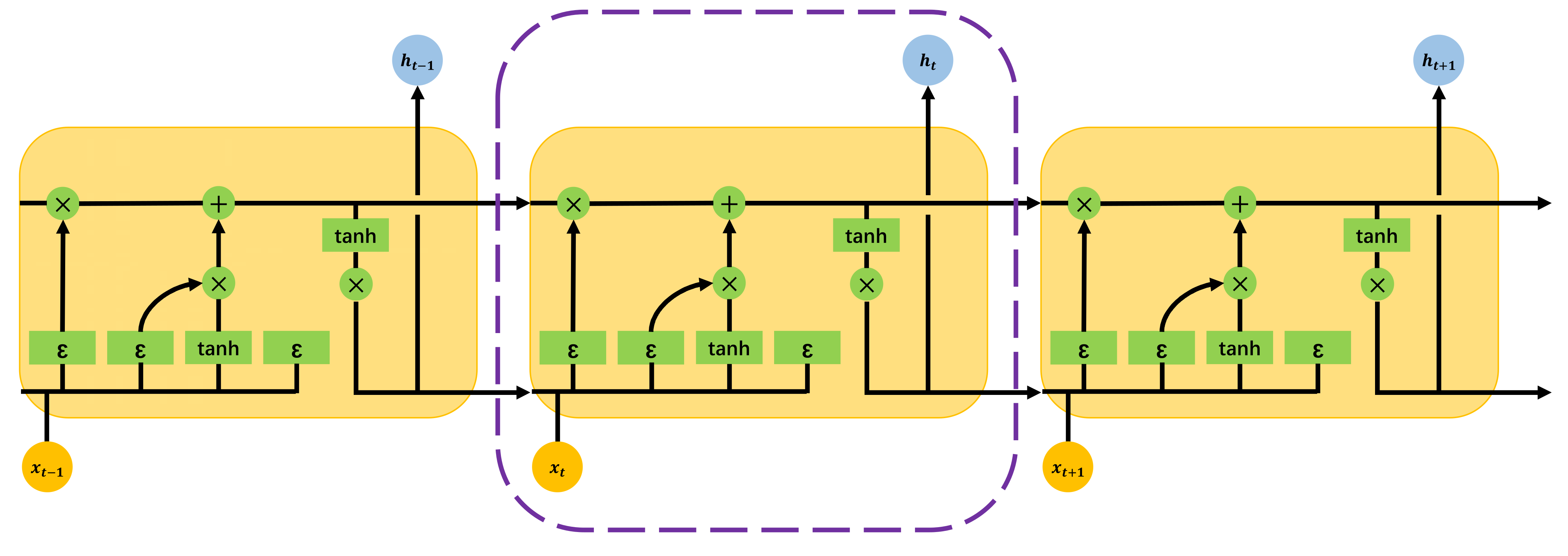
A recurrent neural network is a neural network with memory.
Figure 1 is a structure diagram of a simple recurrent network [
40]. There are five neurons in the input layer, three nodes in the hidden layer and three neurons in the output layer. The structure of an RNN is similar to that of a fully connected neural network [
41,
42]. The main difference is the memory element in the middle. The existence of the memory element makes the output,
y of
n, not only determined by the previous
x but also related to the state of
n in the previous time step. The result of the memory is circulated into the current time step for common operation, and the weight in each connection is determined by the neurons, ω, connected before and after.
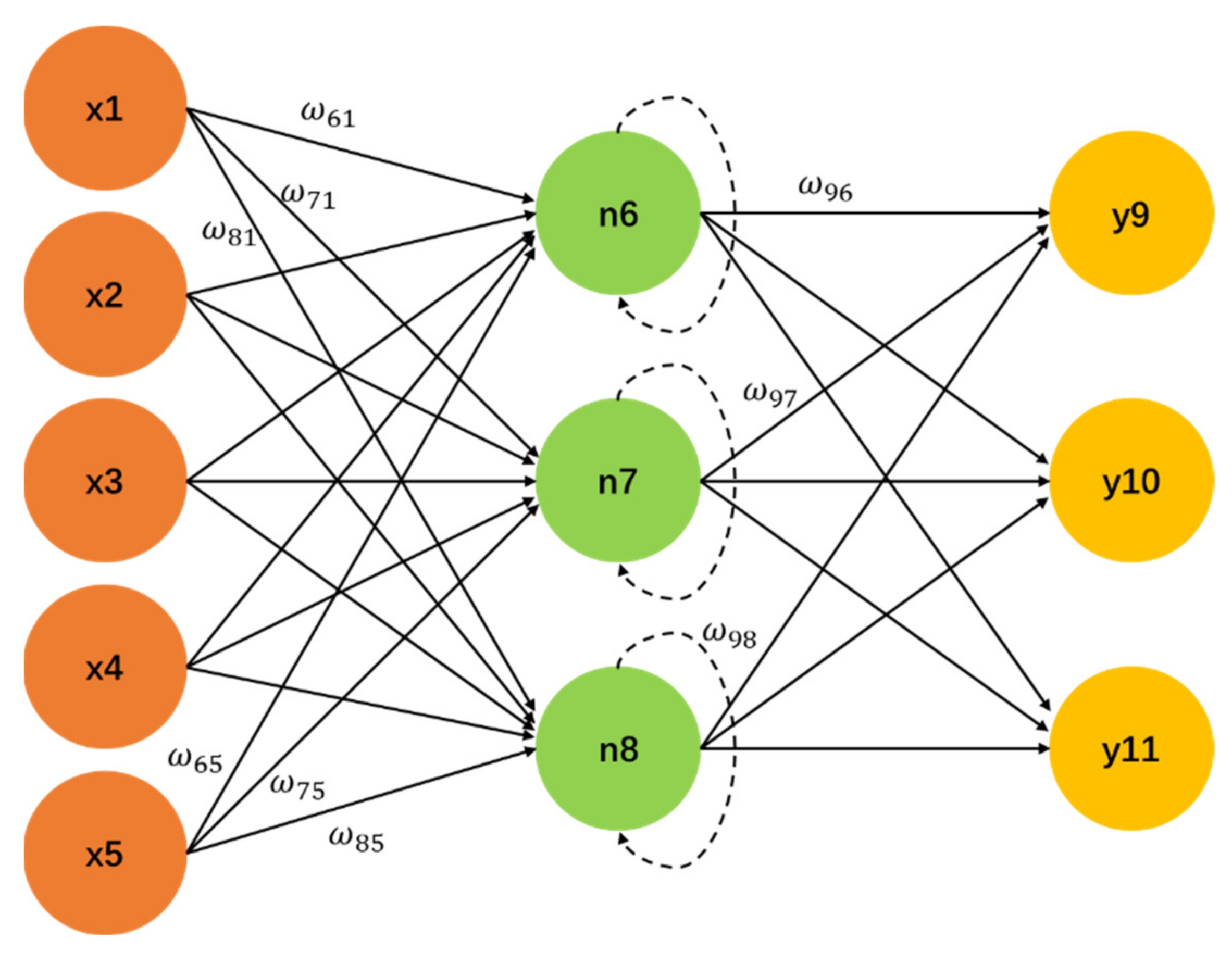
Figure 2 shows the network structure of LSTM. The structure is composed of multiple recurrent units stacked together. The framework of the main part is based on RNN, but the significant difference is that there are some gated technologies in the internal units, that is, forget gates, input gates and output gates. The gating mechanism mainly controls the path of information propagation and improves the ability of the hidden layer to learn deep information. Similar to RNN, the result,
, of the previous time step will be combined with the input,
, of the current time step. After the operation,
will be obtained, and then
will be stored and calculated together with
of the next time step. The method will continue running in this way until the end. ε in the figure represents the sigmoid function, which is used in addition to the tanh function of the hyperbolic tangent in the unit.
The forget gate function is
where
is the weight matrix of the forgetting gate, and
is the bias term of the forgetting gate.
represents the activation function, and
generally takes
as the activation function.
The input gate is used to calculate the data,
, saved to the memory unit at the current time step:
where
represents the weight matrix of the input gate,
is the output of the network at the previous time step,
is the input of the current time step and
is the bias term of the input gate.
The new information,
, saved to the memory unit generated by the transformation of the currently input information is:
The activation function, tanh, in the above formula can limit the result to the [−1, 1] interval, and and are the weight matrix and the bias term, respectively.
The calculation formula of the memory value,
, of the current time step is as follows:
where
represents the Hadamard product. In this equation, the item before the addition sign represents the information filtered through the forget gate, and the latter item represents the new information added.
The information formula output by the output gate is as follows, where
represents the weight matrix of the output gate, and
represents the bias term of the output gate.
The output result,
, of the current time step is:
According to the mechanical relationship of elastic parameters in rock physics, the Lame coefficient conversion formula is:
where
is Young’s modulus, and
is Poisson’s ratio. Young’s modulus and Poisson’s ratio are:
where
; then, we can obtain
according to Equations (24)–(26),
Mapping between reservoir elastic parameters and reservoir attributes can be established using rock physics based on the LSTM network. The data with high resolution and multiple parameters obtained from inversion are fixed with multiangle prestack-angle gathers, and the prior log information is used to establish constraints. The long short-term memory neural network is used to iteratively correct the model until a reservoir property parameter volume with a high coincidence rate is obtained.
3. Results
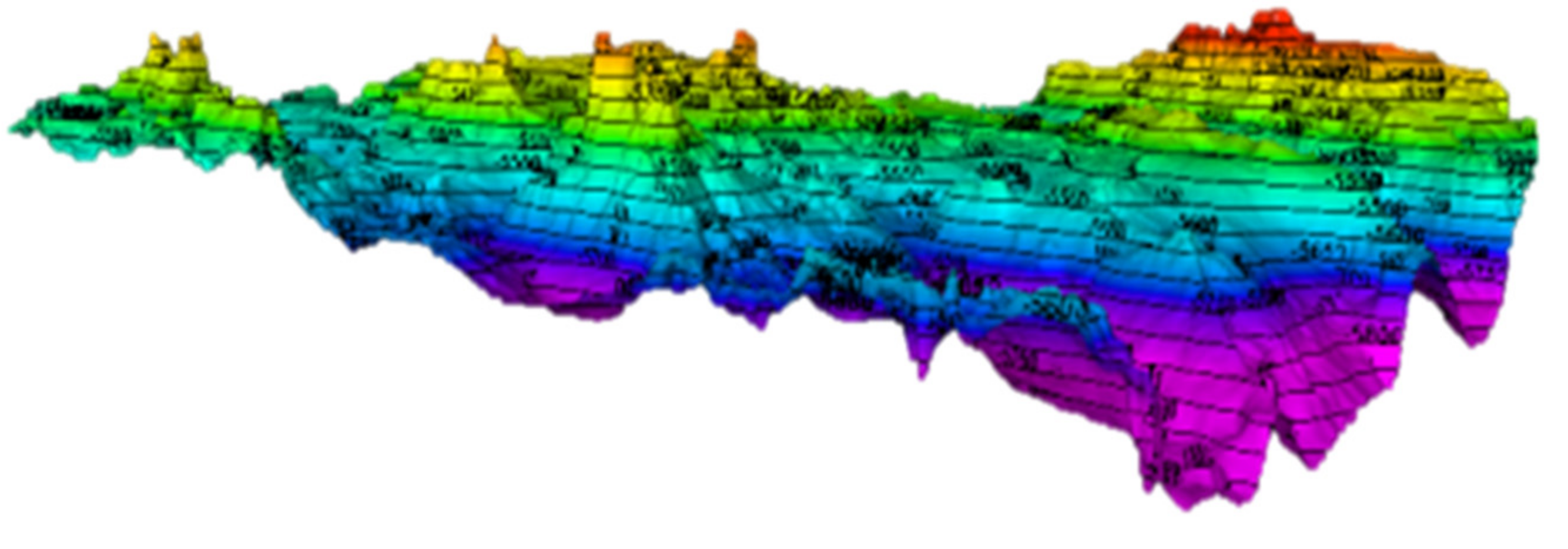
The H Basin has a structural pattern of uplift and depression, as shown in
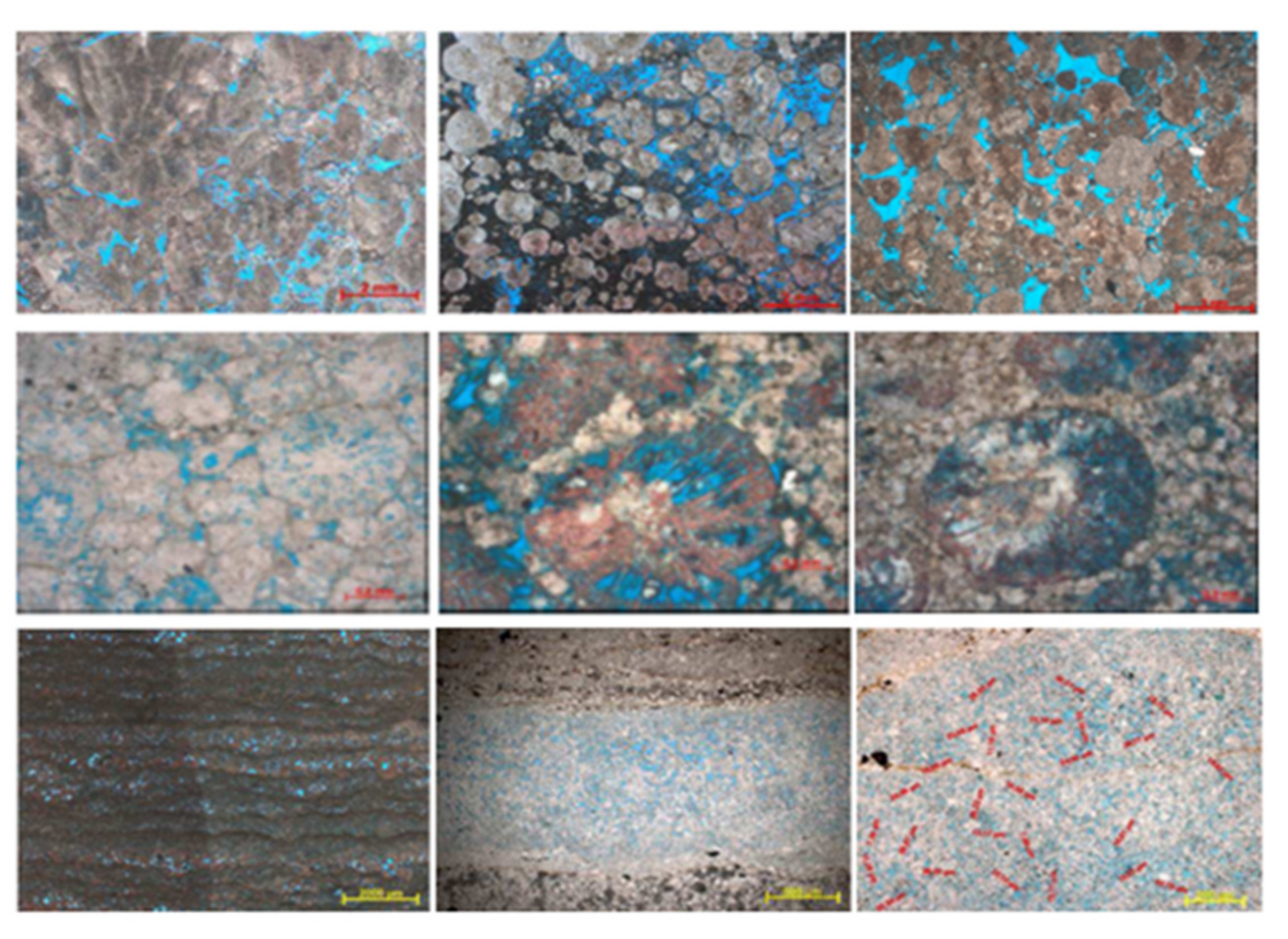
Figure 3. From the shore to the sea, the basin can be divided into three tectonic units: a coastal uplift zone, a sunken zone and a platform. It is a typical passive continental margin salt-bearing basin, which is mainly divided into two oil-gas systems: the presalt system and the postsalt system. The G group of the target interval belongs to the Lower Cretaceous depression sequence. The depth of the target layer is between 5000 and 7500 m, and there is a thick salt rock layer above the target layer. Based on the above geological background, it is confirmed that the working area belongs to a deep-water presalt carbonate reservoir. The main frequency of the seismic data is approximately 14 Hz, and the frequency band is approximately 5–25 Hz. The main frequency belongs to the seismic signal of the low dominant frequency and low frequency bands. The prestack data volumes are stacked into seismic data volumes with three partial-angle gathers in the range of 3–12°, 12–21° and 21–30°. The lithology is complex and diverse. According to the scanning electron microscopy (SEM) analysis of the main reservoirs, as shown in
Figure 4, the lithology of the G1 layer mainly shows high porosity and medium permeability, with distributed stromatolites and granular rocks. The G2 layer mainly shows medium-high porosity and low-medium permeability and is mainly distributed in spherical microbial limestone. The G3 layer is mainly characterized by medium porosity, low permeability and extra-low permeability and is mainly distributed in striated limestone. The focus of this study is on the G1 and G2 layers.
Reef-shoal facies and intershoal depressions are developed in the presalt carbonate rocks in the study area, the reservoir heterogeneity is strong and the lateral variation is large. According to the observation of cores and outcrops, analysis of the geological conditions and prior information, such as sediments, physical parameters and lithology, the reservoirs are divided into three types: type I reservoirs are reefs, type II reservoirs are beaches and type III reservoirs are platform facies, as shown in
Table 1. The reefs mainly develop stromatolites with good reservoir properties and porosities greater than 14%, the beach facies mainly develop grainstone and pellet limestone with porosities of 10% to 14% and medium reservoir properties, and the platform facies mainly develop laminated bindstone with relatively poor reservoir properties and porosities less than 10%.
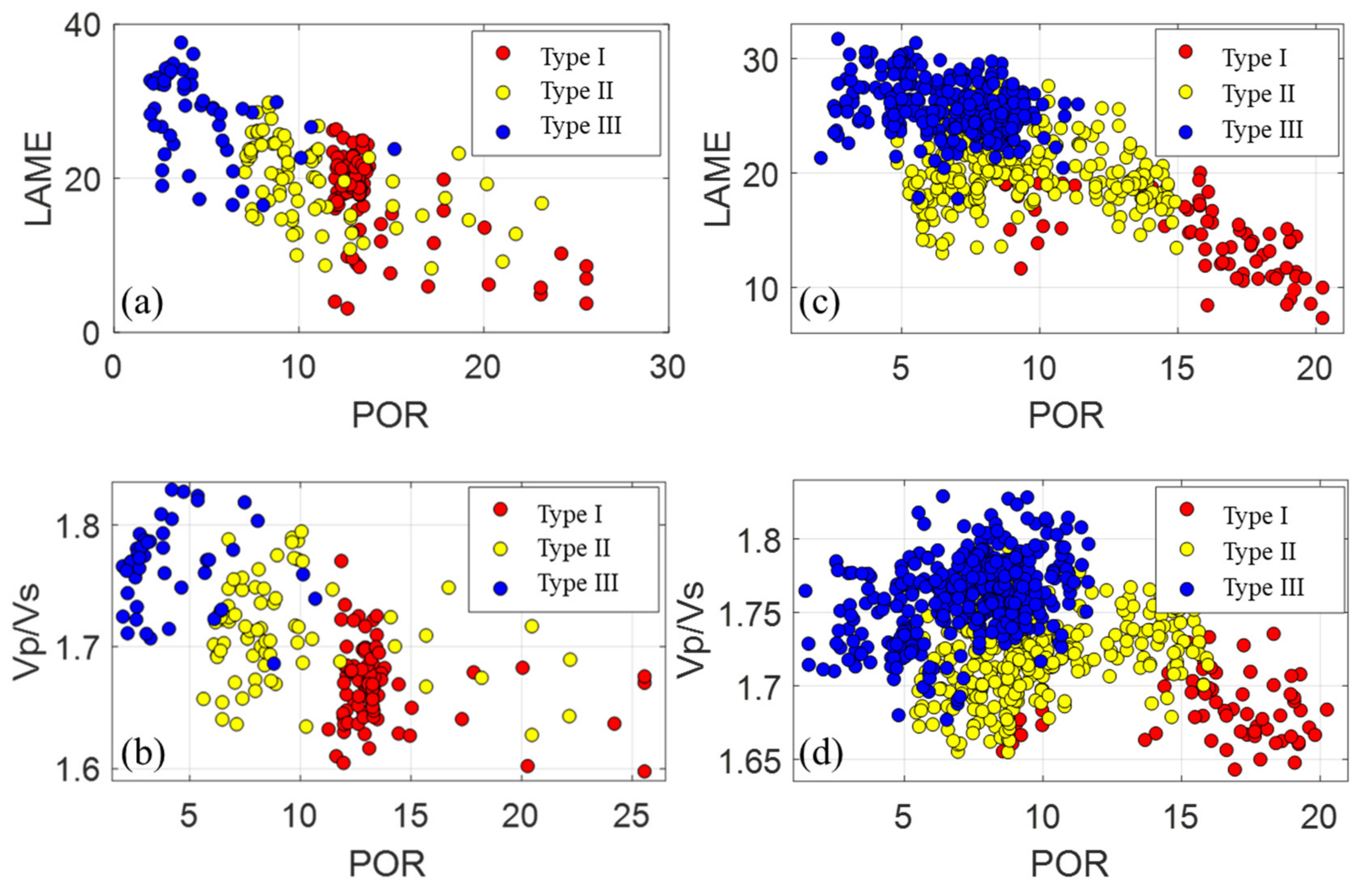
By optimizing the physical parameters of the rock, finally, the G1 and G2 layers can be sufficiently distinguished into type I, type II and type III reservoirs through the intersection of the Lame coefficient and porosity and the intersection of
and porosity, which is less sensitive than the Lame coefficient, as shown in
Figure 5. The rock-physical statistics show that the intersection of porosity and the Lame coefficient can better distinguish the three types of reservoirs. Type I reservoirs show a low Lame coefficient and low
, type II reservoirs show a medium Lame coefficient and medium
, and type III reservoirs show a high Lame coefficient and high
. To obtain the porosity data volume, the relationship between porosity and Lame coefficient must be established. The parameters obtained from the petrophysical analysis can provide relevant parameter constraint thresholds for subsequent multiparameter interactions and reservoir predictions.
Combining the P-wave, S-wave and density log data of the wells in the study area allows for the construction of a low-frequency model. The initial low-frequency model of the prestack three-parameter inversion established by the seismic data is shown in
Figure 6. The initial model established by this method varies in different target intervals. The corresponding low-frequency initial models are different, with highly apparent lateral variation features.
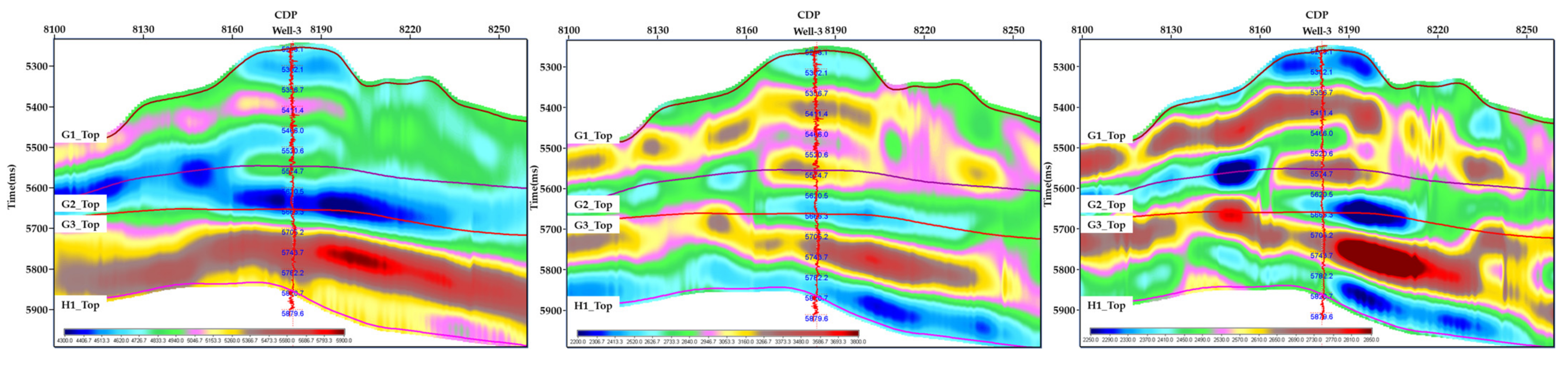
The Lame coefficient inversion results are obtained by using the prestack multiparameter inversion method in the study area.
Figure 7 is the profile of the Lame coefficient results obtained from the actual data inversion in the study area. Well 5 is a new well without shear wave information that does not participate in the prestack inversion work; therefore, Well 5 can be used here for testing of the inversion effect. From the variation of the gamma GR curve and the real resistivity RT curve of the Well 5 section, it can be seen that the reservoir corresponds well to the log curve and the inversion result profile. The Lame coefficient inversion profile is in good agreement with the actual reservoir, which can better characterize the changes in oil-bearing reservoirs.
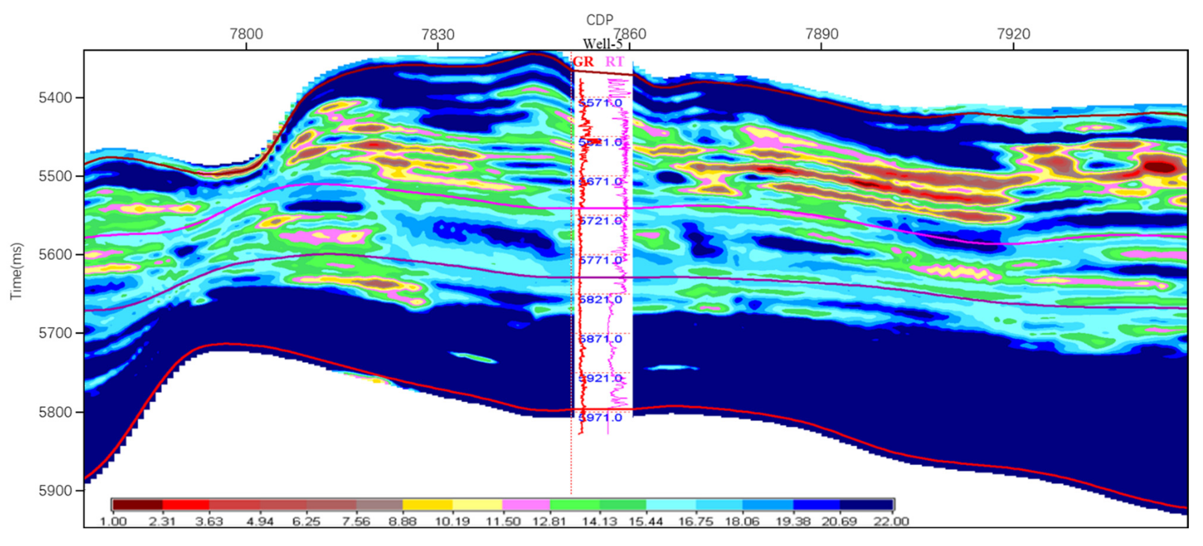
The common inversion method for software used in industry is the simultaneous sparse-pulse inversion method. The two inversion results are compared in
Figure 8. The upper figure is the Lame coefficient inversion profile obtained by constrained sparse-pulse inversion, and the lower figure is the Lame coefficient inversion profile obtained by multiparameter joint inversion. From the
Figure 8, the Lame coefficients can better characterize the change in oil-bearing reservoirs. From left to right, the reservoir varies from thick to thin before thickening again. Although the constrained coefficient pulse inversion can reflect the changing trend of reservoir thickness, it is obvious that the inversion results in the figure below can obtain thinner reservoirs and high-resolution results, which proves that the new inversion method can obtain more accurate inversion results.
The Lame coefficient inversion data volume and seismic and log information obtained by the method in this paper are used as joint prior constraints. Because the magnitudes of the data are different, the input data must be normalized, and the output result is the porosity data volume. The model convergence analysis in this paper adopts the mean square error method the adaptive moment estimation (Adam) algorithm for optimization. The initial learning rate is 0.005. To prevent the gradients from exploding, the gradient threshold is set to 1. During learning, an optimization operator is used to join the neural network so that after a certain training time, the learning rate will be multiplied by a coefficient between 0 and 1; it is expected that more accurate results will be obtained in the later stage of learning. After repeated testing and optimization, the results of the LSTM model test are shown in
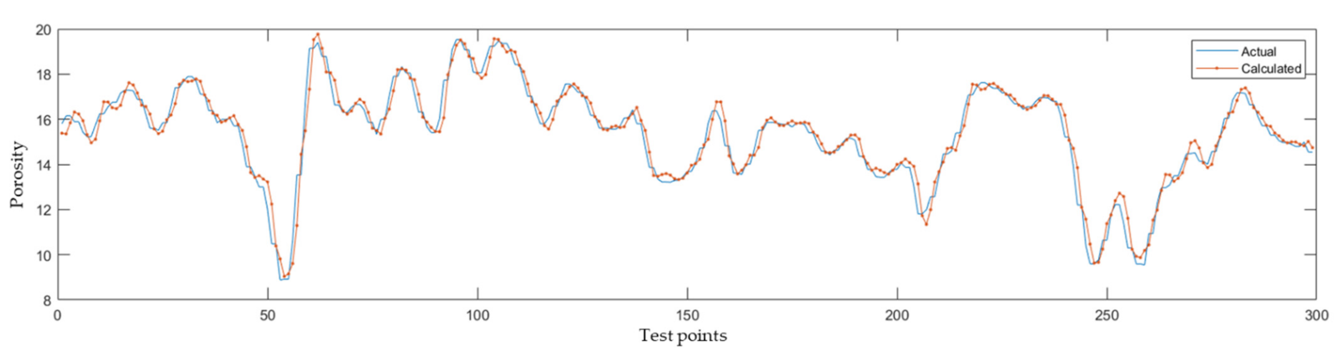
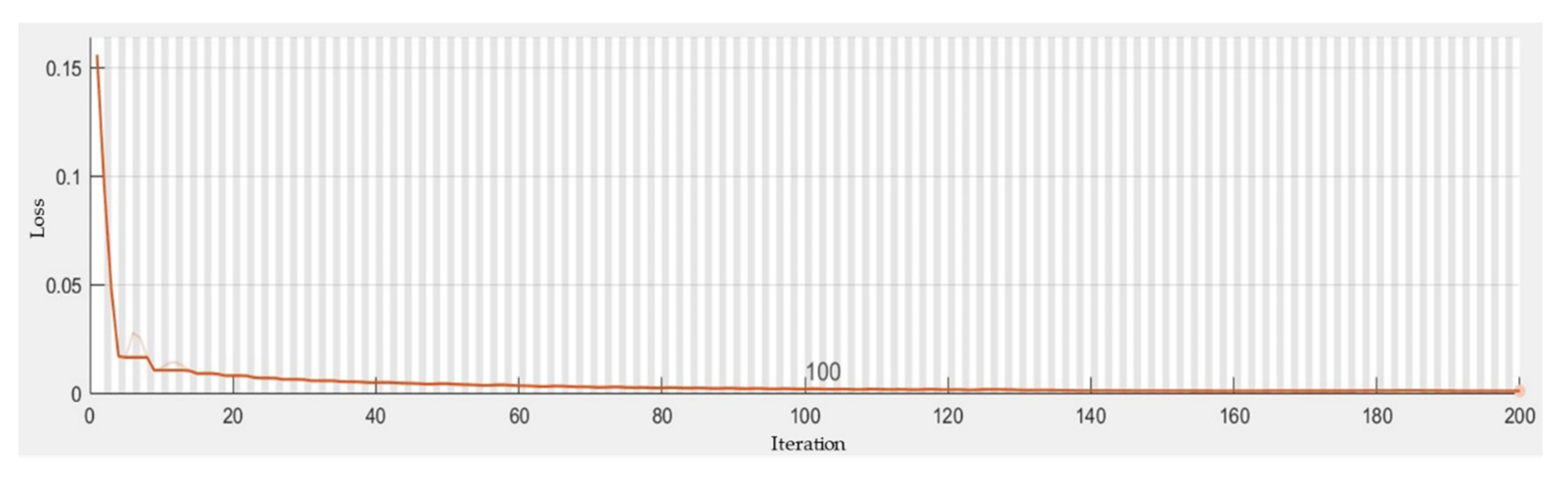
Figure 9. The verified actual data and the model-calculated data exhibit changes with a consistent trend. The training situation of the model is shown in
Figure 10. It can be seen that the model is relatively good after approximately 40 iterations, and the loss is almost stable by approximately 110 iterations.
Table 2 shows the adopted architecture, hyperparameters and errors of the applied LSTM. At this time, the RMSE value is 0.4603, the MSE value is 0.2119 and the R
2 value is 0.9830. The final inversion LSTM network structure consists of one input layer, three hidden layers and an output layer. The number of hidden units is 28, and gradient descent is used for convergence.
To obtain high-precision porosity inversion results, in this article, we use a deep neural network (DNN) based on the backpropagation (BP) algorithm and LSTM network to test the data volume. The BP neural network is a multilayer feed-forward neural network trained by the error backpropagation algorithm. The topological structure of the BP neural network model can be divided into three layers: the input layer, hidden layer and output layer. The model learns according to given input samples and output samples and according to certain training criteria, such as the minimum mean square error. The error between the actual output value and the expected output value of the network is calculated, and error backpropagation is continuously carried out to adjust the weight of each layer of the network to minimize the error and complete the purpose of learning. DNNs based on the BP algorithm are widely used in predictive deep learning frameworks. This model has a very strong nonlinear fitting ability, and it can fit almost any function, so we chose it for comparison in this manuscript.
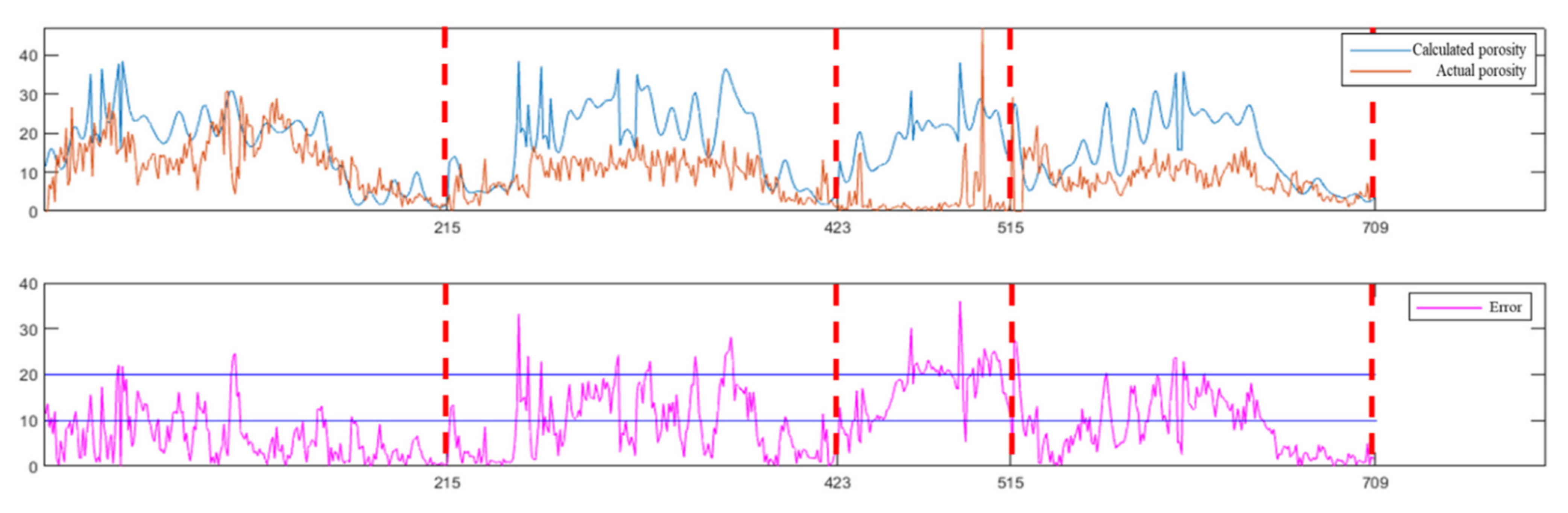
Based on the data for the four new wells, different methods are used for comparison.
Figure 11 is a comparison of the porosity of the four new wells not included in the deep learning activity and with the porosity predicted by the DNN. The blue curve is the porosity calculated by the inversion based on the DNN with the BP algorithm; the light red curve is the actual porosity data, where each segment of the red dotted line represents the information of each well of the four new verification wells; and the purple curve represents the porosity error.
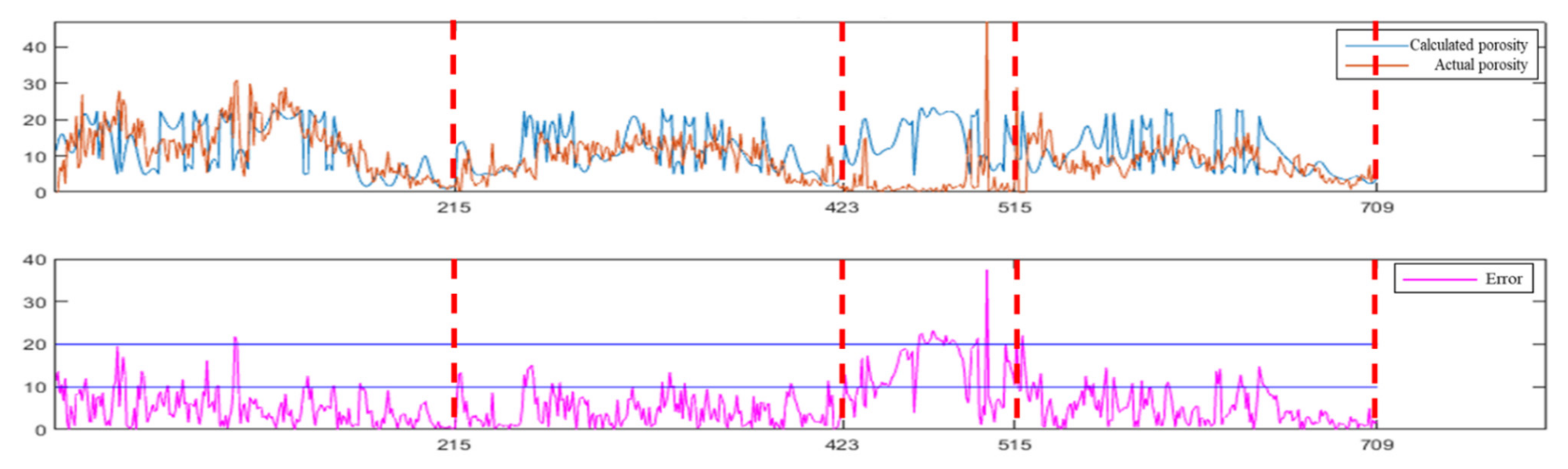
Figure 12 is a comparison of the porosities of the four new wells not involved in deep learning with the porosities predicted by the LSTM network, in which the blue curve is the porosity calculated by inversion based on the LSTM algorithm, the light red curve is the actual porosity data and the purple curve represents the porosity error. Because the third new well with porosity information is a well outside the work area, that is, the well with the abscissa ranging from 423 to 515 in
Figure 11 and
Figure 12, it is mainly used with the three other new wells to reflect the porosity of the two methods. The inversion effect of the porosity is not calculated in the final calculation of the statistical rate in the work area. It can be seen from the comparison results of
Figure 11 and
Figure 12 that the porosity errors of the four wells are reduced. Although DNN can obtain good results and the average porosity coincidence rate obtained by calculation is approximately 89.48%, the porosity inversion results based on the LSTM algorithm have an average porosity coincidence rate of 97.76%, which is better than that of the deep neural network and is more suitable for deep learning inversion in this work area.
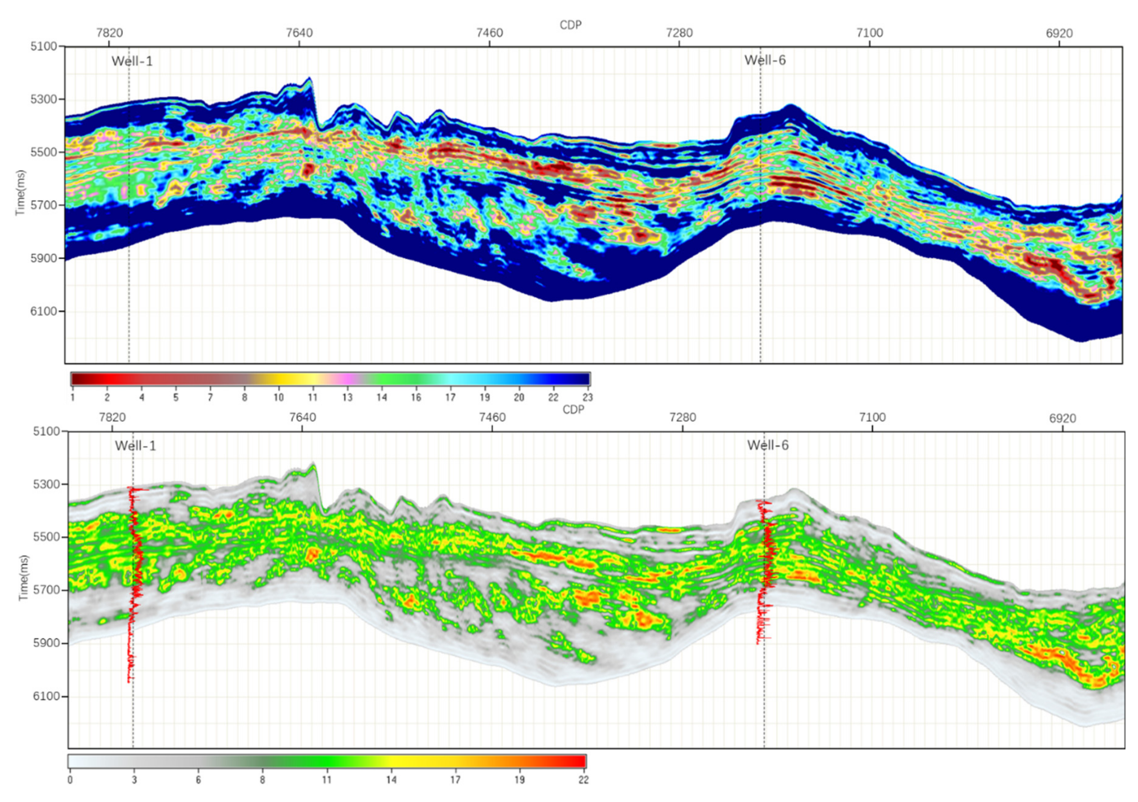
The obtained Lame coefficient inversion data volume, the original logging porosity, the seismic trace gather and other information are used as prior information for deep learning inversion. Based on the Lame coefficient result profile of the multiparameter joint inversion in the upper image of
Figure 13 and the porosity result of the multiparameter joint inversion with LSTM in the lower image, Well 6 has logging porosity data but lacks a constraint inversion process, which is used to verify the accuracy of the porosity inversion data volume. By extracting the well-tie profile, it can be seen that the porosity data volume based on deep learning LSTM are horizontally distributed in layers, and the change in the inversion porosity data volume in the vertical direction at Well-6 is consistent with the changing trend of the porosity logging curve. The porosity inversion profile and the highly sensitive Lame inversion profile have the same change trend, which can better depict the underground geological conditions. From the results of deep learning, the method based on multiparameter joint inversion and LSTM can obtain reasonable prediction results from reservoir parameters.
4. Discussion
When the parameters are solved in reservoir prediction, especially in the case of logged information constraints, the constrained sparse-pulse inversion method is often used, which can better reflect the lateral changes in the reservoir, despite the fact that the resolution of this method is low. When the underground reservoir structure is not so complex or the reservoir is thick, this inversion method can be used for reservoir prediction. However, the multiparameter joint inversion method based on deep learning, as used in this article, can be better applied in the case of carbonate reservoirs under salt, which have a low main frequency and complex underground reservoir structure.
The fitting problem between different parameters is basically low-dimensional. The traditional method is to use Gaussian fitting or polynomial fitting to solve the problem directly. The information that can be used is relatively singular. The use of LSTM in deep learning can obtain better results with greater accuracy. The multiparameter joint inversion method based on deep learning, as proposed in this paper, can improve the accuracy of reservoir prediction and increase the resolution and stability of the inversion results, which improves the consistency of the multiparameter inversion results. The results show that multiparameter joint inversion can reflect the thin-layer changes of the underground structure, which is helpful for a new round of exploration and development of the oilfield in the future and for setting new well positions.
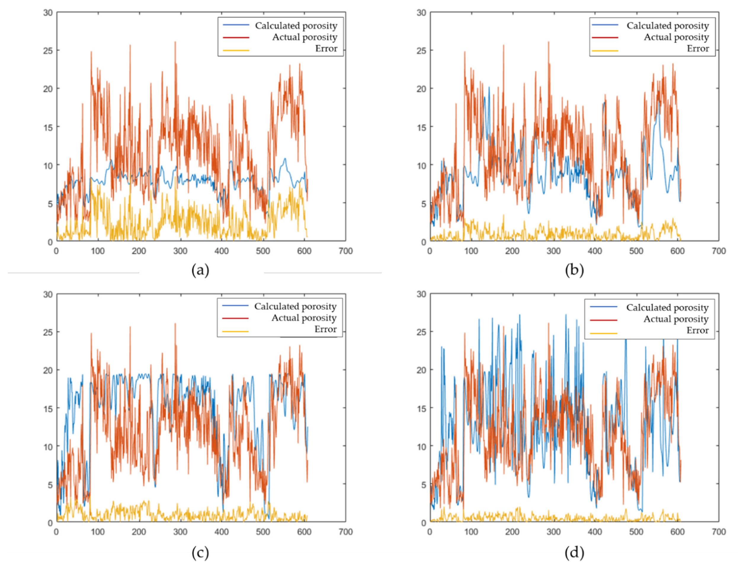
In the network construction process of LSTM based on multiparameter inversion, the selection process of hyperparameters also has an important impact on the final accuracy of porosity prediction. The following discusses four typical examples of hyperparameter tuning processes.
Figure 14a,b shows the results when the learning rate is 0.1 and 0.001, respectively, under the same conditions of other hyperparameters. It can be seen that the calculated porosity and the actual porosity have similar trends, but the error in (a) is much larger than that in (b), and the coincidence rate in (a) is approximately 58.63%. Both (b) and (c) in
Figure 14 are the results of changing the number of LSTM hidden units, whereas the learning rate and other parameters remain unchanged. Among them, the overall coincidence rate of (b) is 91.28%, and the coincidence rate of (c) is approximately 87.40%. It can be seen that changing the number of LSTM hidden units changes the final coincidence rate result, although the impact is not as large as the learning rate. The difference between (d) and (b) is as follows: after setting a better learning rate and number of LSTM units, by setting the dropout factor function, the learning accuracy increases with the number of iterations in the later stage of training. At this time, the coincidence rate of (d) reaches 93.15%. From the discussion of the above examples, it can be concluded that when the network is optimized for hyperparameters, the learning rate has a greater impact on the final result, followed by the number of LSTM hidden units, and the model accuracy can be increased by setting the drop factor, although the impact is smaller than that of the previous two parameters.
Because hyperparameter optimization involves many intrinsic parameters of neural networks, it is an optimization problem of parameter combination, so it cannot be optimized by methods such as gradient descent; thus, there will be great uncertainty in the optimization process. Currently, most of the hyperparameters in the application are manually configured, which is also closely related to the experience of the researchers. Most of the selection process is based on experience and compares multiple results to select the results of the hyperparameters corresponding to the best results. In addition, the optimization of hyperparameters often depends on the quality of the results used to determine the quality of the parameters. However, when faced with a large amount of data, each time, the process of solving for the results takes considerable time, which makes the optimization process of hyperparameters very time-consuming. The above process of hyperparameter selection and optimization needs to be further studied in the future.
The particle swarm optimization method can search several random solutions and then iterate to determine the optimal solution. Particle swarm optimization can be introduced into the hyperparameter optimization process of deep learning to obtain the most suitable hyperparameters for the model. Alternatively, a Bayesian optimization selection method for hyperparameters can also be considered, and the next optimal hyperparameter combination with maximum probability can be predicted according to the existing hyperparameter results. The above two optimization algorithms or similar optimization algorithms obtain results with smaller errors in the construction of a deep learning framework.
Because the LSTM is composed of input gates, output gates and forget gates, the computer used for calculations must meet stronger requirements for calculation efficiency. If the amount of data to be processed is particularly large, some other networks, such as gated recurrent units (GRUs), can also be considered to reduce the calculation load. In this case, fewer parameters can be used in the GRU network, and the proportion of forgetting versus remembering information can be selected by using one gate-control signal. Due to the structural characteristics of LSTM itself, it is difficult to parallelize, although new technologies may serve to optimize it in the future. Therefore, we can also consider using other networks for analysis in the future, which may offer better results.
In the future, we will be able to refer to the new method proposed in this article to solve problems associated with reservoir prediction, going beyond analysis of known carbonate reservoirs, e.g., traditional sandstone reservoirs. If we encounter an oil field during the development period or a work area with significant well information, then due to the increase in prior information and data, the method in this article should be able to obtain better results with greater efficiency than the conventional prediction method.


