Article

Molecular Simulation Study and Analytical Model for Oil–Water Two-Phase Fluid Transport in Shale Inorganic Nanopores

1
School of Petroleum Engineering, China University of Petroleum (East China), Qingdao 266580, China
2
Key Laboratory of Unconventional Oil & Gas Development (China University of Petroleum (East China)), Ministry of Education, Qingdao 266580, China
3
Exploration and Development Research Institute, SINOPEC Shengli Oilfield Company, Dongying 257015, China
4
Key Laboratory on Exploration and Development for Unconventional Oil and Gas of Shandong Province (Preparation), Dongying 257015, China
*
Author to whom correspondence should be addressed.
Energies 2022, 15(7), 2521; https://doi.org/10.3390/en15072521
Submission received: 8 March 2022 / Revised: 25 March 2022 / Accepted: 28 March 2022 / Published: 30 March 2022

Abstract

:
Shale reservoirs contain omnipresent nanopores. The fluid transport phenomena on the nanoscale are significantly different from that on the macroscale. The understandings of fluid transport behavior, especially multiphase flow, are still ambiguous on the nanoscale and the traditional hydrodynamic models are insufficient to describe the fluid flow in shale. In this work, we firstly use a molecular dynamics simulation to study the oil–water two-phase flow in shale inorganic quartz nanopores and investigated the unique interfacial phenomena and their influences on fluid transport in a confined nanospace. The results of the molecular simulation revealed that the water-oil-water layered structure was formed in quartz nanopores. There is no-slip boundary condition between water and quartz surface. The density dip and the extremely low apparent viscosity of the oil–water interface region were observed. The liquid–liquid slip effect happened at the oil–water interface. Based on the nano-effects obtained by the molecular simulation, two mathematical models were proposed to describe the nanoscale oil–water two-phase flow, considering both the solid–liquid and liquid–liquid interfacial phenomena, and the performances of two mathematical models were validated. This study shed light on the flow behaviors of oil and water on the nanoscale, and provides the theoretical basis for scale-upgrading, from the nanoscale to the macroscale.

1. Introduction

Shale reservoirs have huge potential for exploration and development. The technically recoverable shale oil resources are about 70–90 billion tons in China [1] and the shale oil production in the U.S. reached 3.29 × 10⁸ tons in 2018, accounting for about 49% of total oil production in the U.S. [2,3]. However, shale reservoirs contain a larger proportion of microscale and nanoscale pores [4,5]. The physical properties of the fluid in confined nanoscale pores are entirely different from that in bulk conditions [6,7,8]. The special phenomena caused by the confinement effect, such as adsorption [9,10], phase behavior changes [11,12] and slip effect [13,14], played significant roles on fluid transport, which were nonnegligible on the nanoscale. Therefore, how to accurately describe the fluid occurrence state and flow behaviors in shale nanopores, and then consider the nanoscale effect into pore-scale or field-scale simulation to guide shale oil development, has become a huge challenge.
The essence of the microscale effect is the intermolecular interactions. Thus, studying the nanoscale phenomena from the level of intermolecular interactions is the most direct and accurate method. The molecular simulation method has great advantages in studying nanoscale phenomena, since it is based on statistical mechanics and quantum mechanics and calculates the physical and chemical properties by the thermal motions of molecules [15]. It has been widely used in material engineering [16], chemical engineering [17] and biology [18]. In recent years, it has been introduced into petroleum engineering, to investigate the fluid behaviors and interfacial phenomena in the nanoscale pores of shale reservoirs and tight reservoirs [19,20]. The virtual particles and ideal materials [21,22] were commonly used in the early studies of nanoscale fluid flow to reveal the phenomena qualitatively, and then gradually extended to adopt the real minerals of shale/tight reservoirs in recent decades. For the single-phase fluid flow in shale nanopores, Yu et al. [23] studied the methane transport in shale inorganic mineral nanopores and graphene nanopores. Wang et al. [24,25] studied the alkane flow in shale reservoir, with consideration of nanoconfinement effects. The results revealed the positive slip boundary condition of both methane and liquid alkanes in inorganic quartz nanopores. The extremely large slip length was observed at the graphene–liquid interface for methane, water and liquid long-chain alkanes, leading to the fast mass transport of fluid. The connate water and the extra water introduced into the subsurface by hydraulic fracturing during shale oil development resulted in the oil–water two-phase fluid flow in shale nanopores. Therefore, it is necessary to clarify the effects of water on shale oil transport and oil–water two-phase flow behavior. However, the previous studies on gas–water and oil–water two-phase flow in shale nanopores were limited. Ho et al. [26] simulated the flow of methane and water in muscovite nanopores and reported the flow pattern changes of methane and water caused by the increase in driven pressure gradient. Ho et al. [27] also studied the supercritical CO2-induced atomistic lubrication for water flow in a hydrophilic nanochannel by molecular simulation and revealed that the multicomponent interactions can be manipulated to enhance the flow capacity. Qin et al. [28] analyzed the effect of surface roughness on the flow capacities of water-based nanofluid. Xiong et al. [29] constructed a molecular model of methane–water two-phase fluid in illite nanopores and found the local electric fields were induced by the positive potassium layer and negative hydroxyl group, which was conducive to forming the water bridge in the nanopores. Zhan et al. [30] studied the effect of water film on oil transport in laminar flow conditions, in the nanoscale pores of shale inorganic minerals, and modified the mathematically model. Our previous work [31,32] investigated the oil–water two-phase flow behavior in calcite nanopores with various oil mass percentages and analyzed the water effect on oil transport. However, the investigation of liquid interfacial phenomena of oil–water two-phase fluid and its effect on oil–water transport in shale inorganic nanopores was still ambiguous and the characterization of boundary conditions at the liquid–liquid interface was still unclear.
Since the scale of nanopores is extremely small, the static and dynamic properties of fluid on the nanoscale are different from that on the macroscale, so the traditional hydrodynamic model used in conventional reservoirs was insufficient to describe the fluid flow in shale. The molecular simulation method and the nanoconfinement effect on the molecular scale cannot be applied directly into pore-scale flow simulation and reservoir simulation, due to the scale incompatibility of the nanoscale and macroscale. Therefore, incorporating the nanoscale effect into the conventional hydrodynamic mathematical model to describe the flow behavior in the nanoscale is necessary, not only for the enhancement of theoretical foundation, but also to provide support for scale upgrading. Zhang et al. [33] established the mathematical model of single-phase oil flow in shale nanopores, with consideration of the slip effect and adsorption at the solid–liquid interface. Cui et al. [34] predicted the oil–water relative permeability with consideration of solid–liquid slip. Wang et al. [35] and Zhan et al. [30] modified the mathematical model for oil–water two-phase flow considering solid–liquid slip and quantitatively characterized the oil–water two-phase region. Previously, the mathematical models of nanoscale flow have mostly been developed for single-phase flow. Only several mathematical models were proposed for nanoscale two-phase flow and only a part of the nanoconfinement effects has been considered. Since the nanoconfinement effect on oil–water two-phase still requires further investigation and the mechanisms of nanoscale multiphase flow are still ambiguous, the mathematical model for oil–water two-phase flow in shale nanopores should be further improved.
In this study, we firstly build up the molecular model of oil–water two-phase fluid in shale inorganic nanopores and investigate the static properties by equilibrium molecular dynamics (EMD) simulation. The pressure-driven flow is simulated based on external field non-equilibrium molecular dynamics (EF-NEMD) simulation and the dynamic properties of oil and water in a confined nanospace are analyzed. Then, based on the interfacial phenomena observed by molecular simulation, we proposed two mathematical models to describe the oil–water two-phase flow in shale nanopores, which, respectively, considered the phenomena of extremely low apparent viscosity at the oil–water interface region and the liquid–liquid slip at the oil–water interface. The accuracies of these two mathematical models are validated and the effect of liquid–liquid interfacial phenomena on fluid flow in nanopores is discussed. The mathematical models, with consideration of the nano-confinement effects in this work, can be coupled with the meso-scale simulation method [36,37,38,39], such as the Lattice Boltzmann method (LBM) and pore network modeling (PNM), to investigate the pore scale flow behavior.

2. Molecular Simulation

2.1. Model Construction and Simulation

The molecular model of oil and water in shale inorganic nanopores is constructed and all the simulations are conducted by the Large-scale Atomic Molecular Massively Parallel Simulator (LAMMPS) package [40]. The n-octane is used to represent oil. Quartz is one of the most abundant inorganic minerals of shale reservoirs. In this study, the hydroxyl quartz is used as the mineral surface to investigate the oil–water two-phase flow in shale inorganic nanopores. Since the sedimentary rocks are initially saturated by water, the surface of quartz is fully hydroxylated at geologic conditions. The unit cell of quartz is firstly cleaved at { 10 1 ¯ 0 } plane [41,42]. Then, the hydrogen atoms are added to the dangling oxygen atoms of the cleaved quartz surface and the unit cell is duplicated and extended in x and y directions, to obtain the hydroxylated quartz surface, as shown in Figure 1. The lateral size of the quartz surface is 8.84 nm × 5.4 nm. The density of the silanol (Si-O-H) group of the hydroxylated quartz surface is 7.55 site/nm2, which is in the range of crystal chemistry calculations. The ClayFF force field [43] is utilized to model the quartz surface, since the ClayFF force field has been proved to be applicable to describe the interactions of hydroxylated quartz and also performed well in the simulation of solid–fluid interactions between inorganic minerals and alkanes.
In this study, n-octane is used to simply represent shale oil, since the physical and chemical properties of pure n-octane are similar to shale oil. The OPLS-UA force field [44] is used to model the n-octane and the SPC/E force field [45] is used to model the water molecules. The water molecules are kept rigid via the SHAKE algorithm [46] throughout all the simulation processes in this study. The periodic boundary conditions are applied in three directions. The cutoff distance is 1.2 nm and the Lorentz–Berthelot (LB) mixing rule [47] is adopted to compute the interactions between unlike atom groups. The Nosé–Hoover thermostat [48] is used to compute the system temperature. The long-range Coulomb interactions are computed by the particle–particle particle-mesh (PPPM) method [49].
To build up the initial molecular model, the n-octane molecules and water molecules are randomly inserted into the quartz nanoslit. The numbers of n-octane and water molecules are calculated by the pore volume and target oil mass percentage. The vacuum layer of three times the length of the nanoslit is added in the z-direction to eliminate the interactions between upper and lower surfaces, caused by the periodic boundary conditions. The simulation procedures are shown in Figure 2. The constant external force fz is added on all the atoms at the top surface, with the bottom surface fixed to control the pore pressure. Both the top and bottom surfaces are treated as a rigid body in all the simulations. The external force can be calculated by the target pore pressure and temperature, as shown in Equation (1). In this study, the simulation temperature is 343 K and the pore pressure is 30 MPa, which are consistent with subsurface conditions. The pressure control is relaxed for 3 ns with the timestep of 0.1 ps in the NVT ensemble.
f z = p pore × A 69.5 × N wall
where fz is the external force added on the upper surface in kcal·mol−1·Å−1; ppore is the pore pressure in MPa; A is the area of the upper surface in nm2 and Nwall is the total atom number in the upper surface.
After the process of pore pressure control, the pore size and the pore pressure are almost stable. Both quartz surfaces are then fixed and the system is relaxed in the NVT ensemble for 6 ns, with the timestep of 0.1 ps. The trajectory of atoms in the last 3 ns is collected to analyze the static properties of oil and water in quartz nanopores. To simulate the flow properties, a constant external force fex is added on the fluid atoms in x-direction, based on the equilibrium construction. The external force fex is calculated by the driven pressure gradient as:
f ex = p × A yz × L x 69.5 × N fluid
where fex is the external force added on the fluid in kcal·mol−1·Å−1; ∇p is the pressure gradient in MPa·nm−1; Ayz is the cross-section area of yz plane in nm2; Lx is the length in the x-direction in nm; Nfluid is the total atom number of oil and water.
Since the centroid velocity of fluid molecules in x-direction is affected by the driven force in non-equilibrium molecular simulation, instead of only the molecular thermal velocity, the thermostat is only coupled in the y-direction, to eliminate the influences of driven forces on temperature computation. The non-equilibrium molecular simulation is conducted in the NVT ensemble for 15 ns and the trajectory of the last 6 ns is collected to analyze the dynamic properties of oil and water in quartz nanopores.

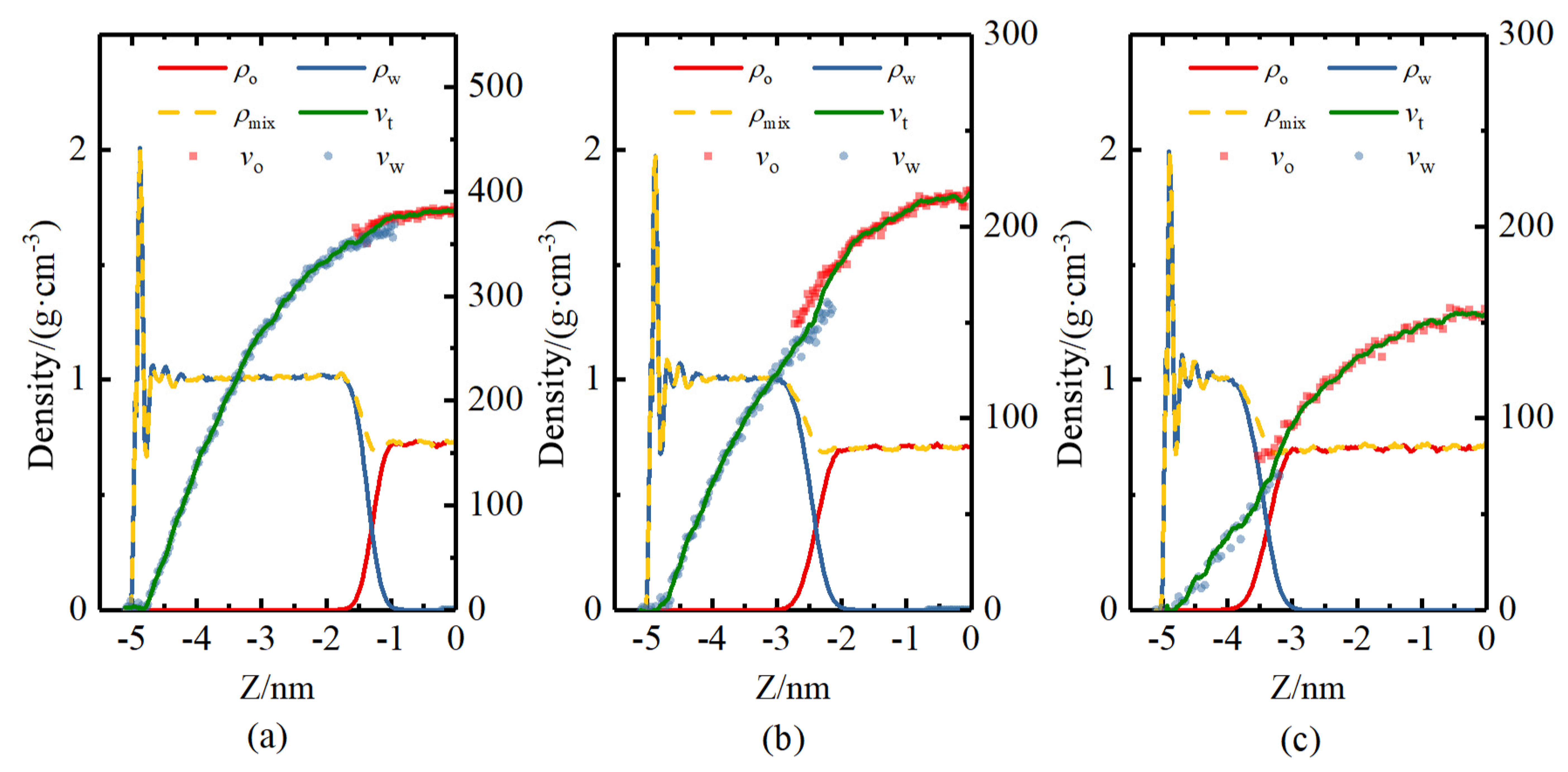
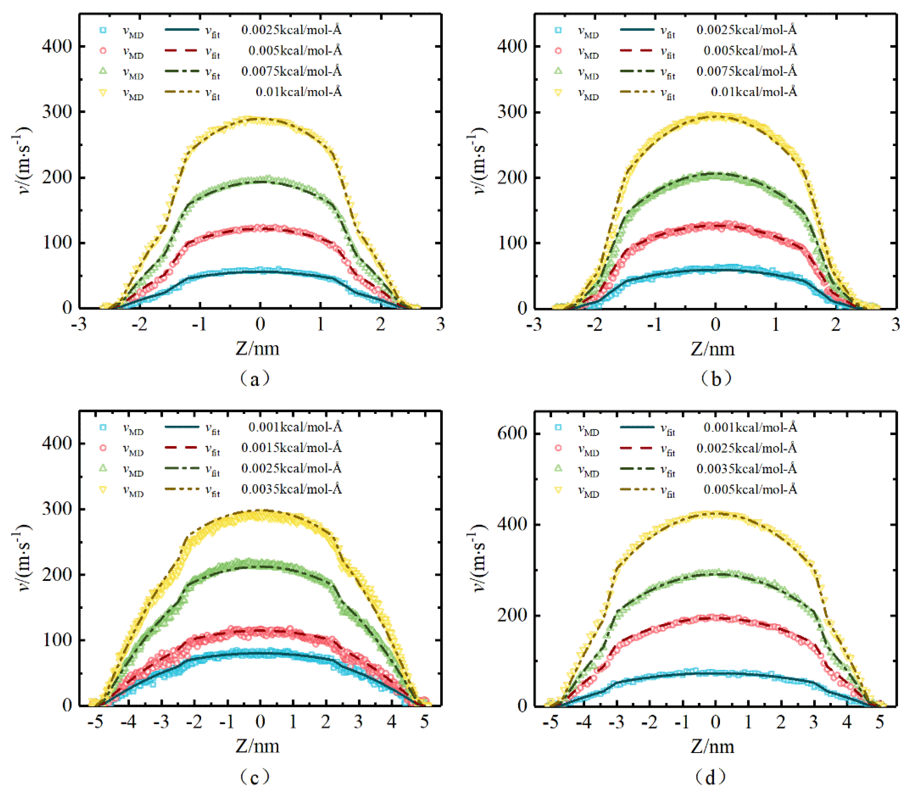
2.2. Results of Molecular Simulation

In this section, we analyze the static and dynamic properties of the oil–water two-phase fluid in quartz nanopores. The equilibrium configuration of oil and water in 5 nm quartz nanopores, with oil mass percentage (OMP) of 50%, is shown in Figure 3 as the example. The layered structure of water–oil–water is formed in quartz nanopores. To characterize the occurrence state of oil and water more accurately and intuitively, we present the density profiles and orientation order parameters of oil and water in 5 nm quartz nanopores in Figure 4. The orientation order parameter refers to the preferential orientation of the molecules, which is defined as [50,51]:
S ( z ) = 3 2 cos 2 θ 1 2
where θ is the angle between the molecule axis and the normal direction of the surface (z-direction). For long-chain alkanes, θ refers to the angle between the head-to-tail line of the molecule and z-direction. For water, the molecule axis is defined as the line between the middle point of two hydrogen atoms and the oxygen atom. The orientation order parameter is dimensionless and ranges from −0.5~1. S = 0 means that the molecules tend to be randomly distributed. Negative S indicates the orientation of molecules preferentially perpendicular to the surface, while positive S indicates the orientation preferentially parallel to the surface.
As shown in Figure 4, since the wettability of the quartz surface is hydrophilic, water preferentially forms multilayer adsorption near the surface. The density of the first adsorption layer is about 2.2 g/cm3. The orientation order parameter at the water adsorption layer is close to −0.5, which indicates the water molecules are preferentially perpendicular to the quartz surface. n-octane is in the center of the pore and demonstrates no adsorption phenomena, since the water film shielded the intermolecular interactions between the n-octane and quartz surface. The orientation order parameter of n-octane is almost stable at 0, which represents no obvious dominant orientation of n-octane. With the position close to the center of the pore, the density of the water phase gradually decreases to 0 and the density of the oil phase gradually increases, forming an oil–water interface region. There is no unified standard for the characterization of the liquid–liquid interface region of two immiscible liquids at present. The commonly used flow region division methods are the 1–99 method [52] and the 10–90 method [53,54], which separate the flow region by the 1–99% of liquid bulk density and 10–90% of liquid bulk density, respectively. In this study, we used the 10–90 method to mark the oil–water interfacial region. The width of the oil–water interface region is ~0.365 nm. The orientation order parameter of both water and n-octane decreases at the oil–water interface region and is close to −0.2, which demonstrates that both water and n-octane molecules are orientated and affected by the intermolecular interactions between each other. Since the intermolecular interactions between water and n-octane are much weaker than that between quartz and liquid, the preferential orientation is less obvious compared with the adsorption layer near the quartz surface.
The total density of the mixed fluid appears to be depressed at the interface, and the fluid density at the interface region is less than single-phase water density and single-phase n-octane density. A similar phenomenon has been reported at the interface of two immiscible fluids in unconfined bulk conditions [55]. Koplik et al. [55] adopted δ, the differences between the average bulk density of two immiscible fluids and the density of the interface region, to quantitatively describe the “density dip” at the interface and the value of δ was only determined by the intermolecular interactions between two immiscible fluids. The overall intermolecular interaction between two fluids is repulsive when two liquids are immiscible, while the overall intermolecular interaction is attractive when two liquids are miscible. The value of δ decreases with the increase in miscibility of two liquids, until no “density dip” appears when the two liquids are completely miscible.
Based on the equilibrium configuration, we investigated the flow behaviors of oil and water in quartz nanopores by adding the constant external force on all fluid atoms in the x-direction. The density and velocity profiles of oil and water in 5 nm quartz nanopores are shown in Figure 5. The density profiles of oil and water during fluid flow are highly consistent with that of a static equilibrium configuration, which demonstrates that the density distributions are not affected by the driven pressure gradient. This phenomenon has also been proved in our previous work, for both single-phase and multi-phase flow [31]. Since the quartz surface is hydrophilic, there is no positive slip observed at the quartz–water interface. The pink and blue dots are the velocity distributions of oil and water obtained by the molecular simulation, respectively. The velocity of oil and water can be fitted by the 2nd order polynomial equation v = a z 2 + c , which is consistent with the Navier–Stokes equations and conforms to the characterization of Poiseuille flow. The green dashed line is the velocity fitting result of the bulk oil region. The apparent viscosity of the bulk oil region in this system can be calculated by the driven pressure gradient and fitting parameter a as [56]:
η app = p / 2 a  
The calculated apparent viscosity of the bulk oil region is about 0.470 mPa·s, which is perfectly consistent with the bulk oil viscosity in unconfined conditions with the same temperature and pressure [57]. The velocity discontinuity appears at the oil–water interface and the oil velocity is slightly higher than water velocity, which indicates the slip phenomenon also exists at the liquid–liquid interface. In previous studies, the liquid–liquid slip has been observed at the interface of two polymers in the bulk condition by experiments [58] and molecular simulation [59,60]. The liquid–liquid slip velocity vs,l refers to the difference between the oil and water velocity, extrapolated linearly from two boundaries of the interface region to the center of the oil–water interface region. The liquid–liquid slip velocity is 3 m/s in this case. The “density dip” is observed at the oil–water interface region, both in static and flow conditions, leading to a reduction in the shear stress at the interface. The apparent viscosity of the oil–water interface region, fitted by the Poiseuille equation, is about 0.196 mPa·s, which is only 0.4 times of the bulk viscosity of n-octane with the same temperature and pressure. The extremely low viscosity of the oil–water interface region would affect the fluid transport in confined nanoscale pores.
The velocity profile of the fluid in 5 nm quartz nanopores, under various driven pressure gradients, is shown in Figure 6. The flow velocity increases with the increase in the driven pressure gradient. The rapid velocity changes are observed as the liquid–liquid interface for all cases. We calculated the apparent viscosity of the bulk-like oil region, bulk-like water region and oil–water interface region, under various driven pressure gradients, by fitting the velocity profiles of each region. The apparent viscosity of the interface region are all ~0.2 mPa·s and the apparent viscosity of the bulk-like oil region and bulk-like water region are all similar, with unconfined bulk oil and water viscosity under various driven pressure gradients, which indicate the apparent viscosity of each region is not affected by the driven pressure gradient. The solid–liquid boundary conditions are not affected by the driven pressure gradient. Our previous work investigated the oil–water flow in calcite nanopores and found the liquid–liquid interfacial phenomena only related to the properties of two liquids. Comparing the flow in the nanopores with various mineral types, we can also confirm that liquid–liquid interfacial phenomena are not affected by the mineral types.
Figure 7 shows the comparison of flow velocity distributions of oil and water in 5 nm quartz nanopores, with various oil mass percentages. The equivalent driven pressure gradient is the same in three various OMP systems. The liquid–liquid slip velocities at the oil–water interface, in various OMP systems, are different under the same equivalent driven pressure gradient. In previous studies, Razavi et al. [61] adopted Lennard-Jones (LJ) fluid to investigate the hydrodynamic phenomena at the liquid–liquid interface. The results show the liquid–liquid slip velocity is related to the fluid types and is positively correlated with the shear stress at the interface. Fang et al. [62] also observed the liquid interface slip in the Couette flow in nanopores and the slip velocity related with the thickness of the wetting phase near the surface. To quantitatively characterize the liquid–liquid slip effect, Equation (5) is introduced to calculate the liquid–liquid slip velocity:
Δ v s , l = α τ
where Δvs,l is the liquid–liquid slip velocity in m/s; τ is the shear stress in MPa; α is the liquid–liquid slip coefficient in MPa·s·m−1, which is only related to the physical properties of two fluids.
The shear stress in this study can be calculated by:
τ = μ eff ,   nC 8 v nC 8 z
where μ eff , nC 8 is the viscosity of n-octane in mPa·s. The oil viscosity is adopted to calculate the shear stress, since the oil phase is in the center of the pore, avoiding the influences of solid surface and the oil layer is thick enough to reduce the calculation error.

3. Mathematical Model

In this section, two oil–water two-phase mathematical models in shale inorganic nanopores are proposed, based on the phenomena observed by molecular simulation. The solid–liquid boundaries and the liquid–liquid interfacial phenomena are taken into consideration.

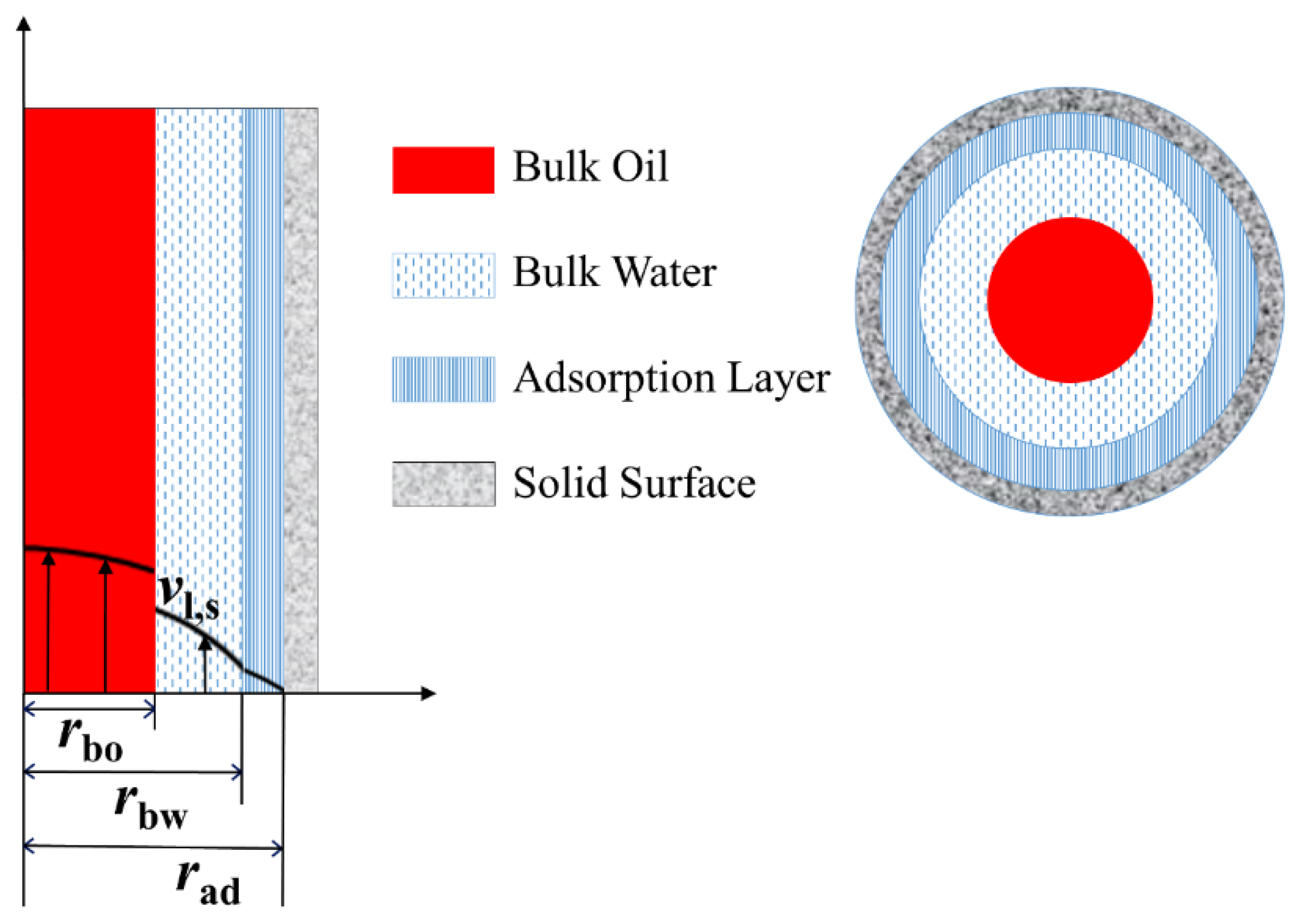
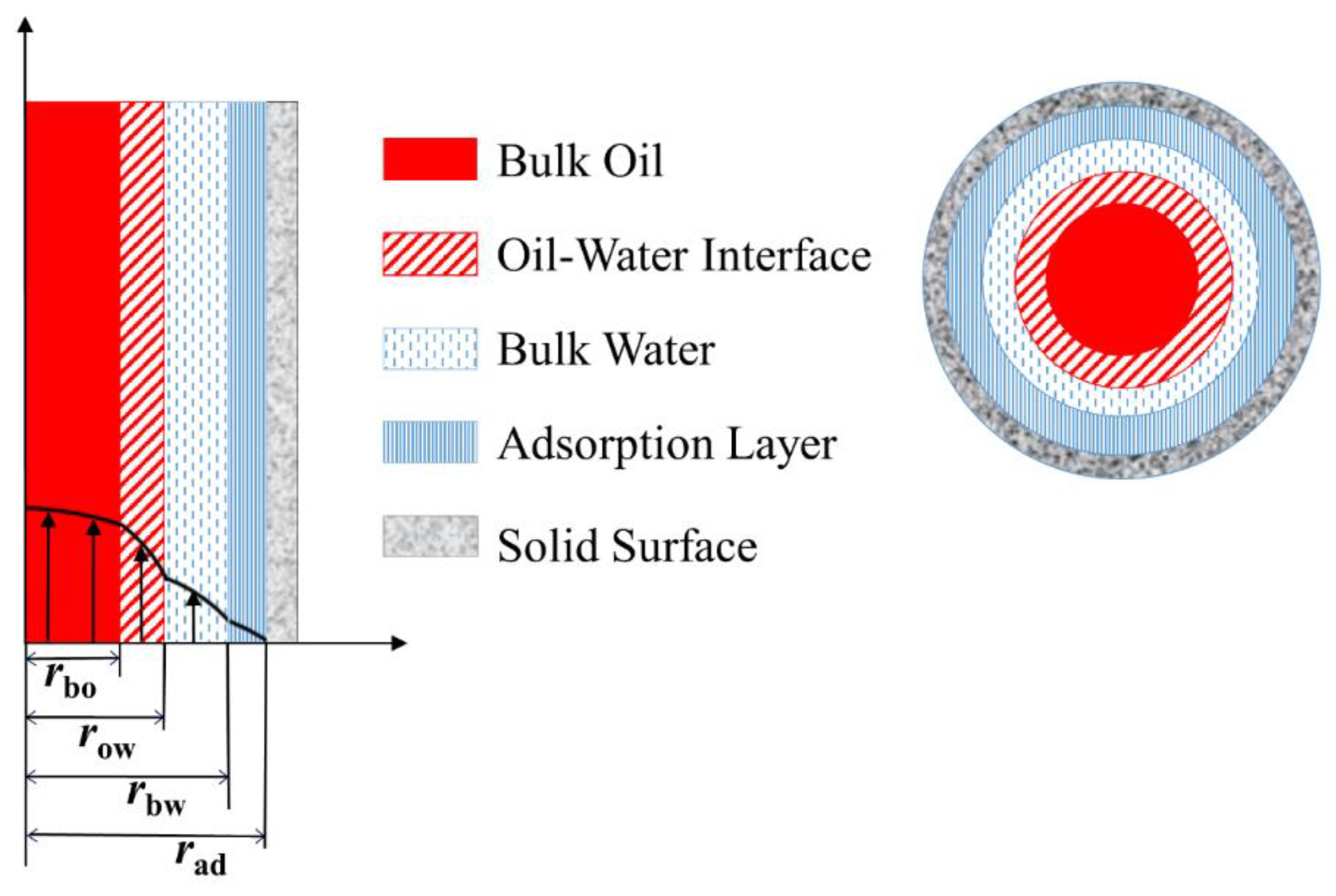
3.1. Liquid Slip Model

The results of the molecular dynamics simulation of oil–water two-phase fluid flow in shale nanopores indicate that the liquid–liquid slip velocity exists at the oil–water interface, while the solid–liquid slip phenomena exist near the pore wall. The flow velocities and flow rates would be underestimated, especially for the non-wetting phase in the center of the pore, without considering the liquid–liquid slip and solid–liquid slip in nanoscale pores.
To model the oil–water two-phase flow in nanopores more accurately, we propose a mathematical model considering the nano-confinement effects, including adsorption, solid–liquid slip and liquid–liquid slip. The basic assumptions of the mathematical model are: (1) fluids are all incompressible; (2) laminar flow and under steady-state condition; (3) no chemical reactions and chemical interactions. The oil–water two-phase flow can be separated into three flow regions: adsorption region, free water region and oil region, as shown in Figure 8. r = 0 is the center of the cylindrical tube and the cross-section of the flow region is symmetric about r = 0.
The governing equation of each flow region can be expressed as:
μ ad r r ( r v ad r ) = p z ,   r [ r bw , r ad ]
μ bw r r ( r v bw r ) = p z ,   r [ r bo , r bw ]
μ bo r r ( r v bo r ) = p z ,   r [ 0 , r bo ]
The boundary conditions of each region follow the conservation of flow velocities, the continuity of the shear stress and the conservation of mass. The solid–liquid boundary condition is a slip boundary, and the slip length can be computed by the contact angle as [63]:
l st = 0.41 ( 1 + cos θ ) 2
Considering the liquid–liquid slip at the oil–water interface, the boundary conditions are expressed as follows:
  v bo r | r = 0 = 0 ;
  μ bo v bo r | r = r bo = μ bw v bw r | r = r bo ;
  μ bw v bw r | r = r bw = μ ad v ad r | r = r bw ;
  v bo | r = r bo = v bw | r = r bo + v s , l ;
  v bw | r = r bw = v ad | r = r bw ;
l st ( v ad r ) r = r ad = v ad | r = r ad
where, lst is the slip length between solid–liquid interface, µad, µbw, µbo are the viscosities of the adsorption region, bulk water region and bulk oil region, vad, vbw, vbo are the velocities of the adsorption region, bulk water region and bulk oil region, vs,l is the liquid–liquid slip velocity.
Combining the governing equation and boundary conditions, the velocities of each flow region can be obtained respectively.
v bo = [ 1 4 μ bo ( r bo 2 r 2 ) + 1 4 μ bw ( r bw 2 r bo 2 ) + 1 4 μ ad ( r ad 2 r bw 2 ) + r ad 2 μ ad l st ] Δ p L + v s , l
v bw = [ 1 4 μ bw ( r bw 2 r 2 ) + 1 4 μ ad ( r ad 2 r bw 2 ) + r ad 2 μ ad l st ] Δ p L
v ad = [ 1 4 μ ad ( r ad 2 r 2 ) + r ad 2 μ ad l st ] Δ p L
where Δp/L is the pressure gradient with the pore length of L.
The fluid flow rate of each flow region then can be calculated by integrating the velocity distribution over the radius in each region.
The flow rate of the adsorption region Qad is:
Q ad = π p 8 μ ad L [ ( r ad 2 r bw 2 ) ( r ad 2 r bw 2 + 4 r ad l st ) ]
The flow rate of the bulk water region Qbw is:
Q bw = π P 8 L { ( r bw 2 r bo 2 ) [ 1 μ bw ( r bw 2 r bo 2 ) + 1 μ ad ( 2 r ad 2 2 r bw 2 + 4 r ad l st ) ] }
The flow rate of the bulk oil region Qbo is:
Q bo = π P 8 L { r bo 2 [ 1 μ bo r bo 2 + 1 μ bw ( 2 r bw 2 2 r bo 2 ) + 1 μ ad ( 2 r ad 2 2 r bw 2 + 4 r ad l st ) ] } + π v s , l r bo 2

3.2. Apparent Viscosity Model

From the molecular simulation, we found that the apparent viscosity of the oil–water interface region is extremely low. Therefore, based on the various apparent viscosities of the different flow regions, we proposed another mathematical model by separately calculating the fluid flow velocity of various flow regions by the apparent viscosity of each region. For the typical water–oil–water layered structure in shale inorganic nanopores, the flow regions are divided into four parts, which are adsorption region, free water region, oil–water interface region and free oil region, as shown in Figure 9.
The governing equation for various flow regions can be expressed as:
μ r r ( r v r ) = p z
The solid–liquid boundary conditions are the same as the “liquid slip model”. Considering the viscosity variety of different flow regions, the boundary conditions of other flow regions all follow the mass conservation, shear stress continuity and velocity continuity, which can be expressed as:
  v bo r | r = 0 = 0 ;
  μ bo v bo r | r = r bo = μ ow v ow r | r = r bo ;
  μ ow v ow r | r = r ow = μ bw v bw r | r = r ow ;
  μ bw v bw r | r = r bw = μ ad v ad r | r = r bw ;
  v bo | r = r bo = v ow | r = r bo ;
  v ow | r = r ow = v bw | r = r ow ;
  v bw | r = r bw = v ad | r = r bw
where, µad, µbw, µow, µbo are the viscosities of the adsorption region, bulk water region, oil–water interface region and bulk oil region, vad, vbw, vow, vbo are the velocities of the adsorption region, bulk water region, oil–water interface region and bulk oil region.
Combining the governing equation and the boundary conditions, the velocity distribution of each flow region can be solved as:
The velocity of the bulk oil region r [ 0 , r bo ] is
v bo = [ 1 μ bo ( r bo 2 r 2 ) + 1 μ ow ( r ow 2 r bo 2 ) + 1 μ bw ( r bw 2 r ow 2 ) + 1 μ ad ( r ad 2 r bw 2 ) + 2 r ad μ ad l st ] Δ p 4 L
The velocity of the oil–water interface region r [ r bo , r ow ] is
v ow = [ 1 μ ow ( r ow 2 r 2 ) + 1 μ bw ( r bw 2 r ow 2 ) + 1 μ ad ( r ad 2 r bw 2 ) + 2 r ad μ ad l st ] Δ p 4 L
The velocity of the bulk water region r [ r ow , r bw ] is
v bw = [ 1 μ bw ( r bw 2 r 2 ) + 1 μ ad ( r ad 2 r bw 2 ) + 2 r ad μ ad l st ] Δ p 4 L
The velocity of the adsorption region r [ r bw , r nw ] is
v ad = [ 1 μ ad ( r ad 2 r 2 ) + 2 r ad μ ad l st ] Δ p 4 L
The volumetric flow flux can be obtained by integrating the velocity distribution of each region over the radius of each region as:
Q ad = r bw r ad v ad 2 π r d r = π p 8 μ ad L z [ ( r ad 2 r bw 2 ) ( r ad 2 r bw 2 + 4 r ad l st ) ]
Q bw = π p 8 L z { ( r bw 2 r ow 2 ) [ 1 μ bw ( r bw 2 r ow 2 ) + 1 μ ad ( 2 r ad 2 2 r bw 2 + 4 r ad l st ) ] }
Q ow = π P 8 L { ( r ow 2 r bo 2 ) [ ( r ow 2 r bo 2 ) μ ow + ( 2 r bw 2 2 r ow 2 ) μ bw + ( 2 r ad 2 2 r bw 2 + 4 r ad l st ) μ ad ] }
Q bo = π p 8 L z r bo 2 [ r bo 2 μ bo + ( 2 r ow 2 2 r bo 2 ) μ ow + ( 2 r bw 2 2 r ow 2 ) μ bw + ( 2 r ad 2 2 r bw 2 + 4 r ad l st ) μ ad ]

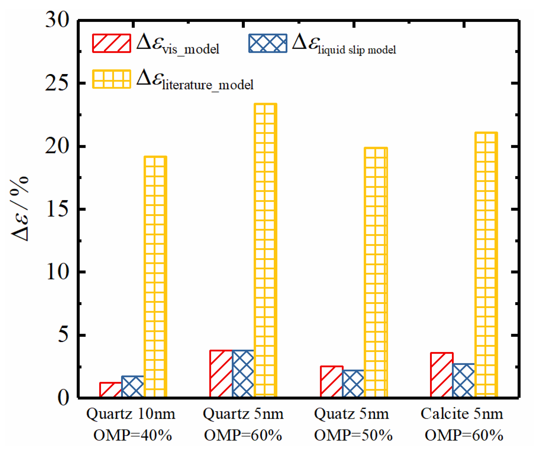
4. Model Validation and Discussion

To verify the feasibility of the mathematical models proposed in this study, we compared the velocity profiles predicted by our model with the mathematical model developed by Cui et al. [34], which only considered the solid–liquid interface without considering liquid–liquid interfacial phenomena (marked as “literature model” in the plot), and also verified this by comparing it with the molecular simulation results. Cui’s model adopted the solid–liquid slip length to quantitatively characterize the solid–liquid boundary condition, while the velocity continuum was assumed at the liquid–liquid interface.

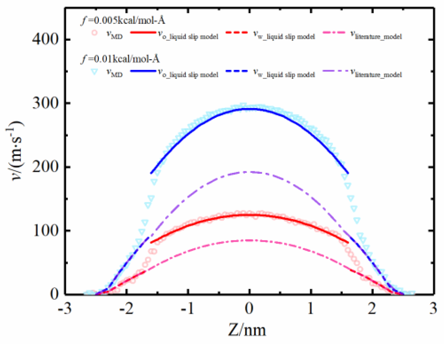
4.1. Model Validation of Liquid–Liquid Slip Model

Figure 10 presents the comparison of the velocity distribution predicted by the “liquid–liquid slip” model and predicted by the model without considering liquid–liquid interfacial phenomena in 5 nm quartz nanopores, under different driven forces. The results show that the velocity predicted by the “liquid–liquid slip” model fitted well with the velocity profile obtained by the molecular simulation. The velocity predicted by the mathematical model, without considering liquid–liquid interfacial phenomena, is significantly underestimated for the velocity of the non-wetting phase in the center of the pore, and the error increases with the increase in driven pressure gradient. Figure 11 is the comparison of velocity profiles, computed by the liquid slip model and molecular simulation results. We adopted several different systems, with various pore sizes, driven pressure gradients and oil mass percentages. The results show that the velocities calculated by the “liquid–liquid slip” model agree well with the molecular simulation results, in all cases, which confirms the feasibility of this model in different conditions. Therefore, considering liquid–liquid interfacial phenomena is necessary for the mathematical model of nanoscale multiphase flow. The comparison results also confirmed the feasibility and the accuracy of the “liquid–liquid slip” model proposed in this study.

4.2. Model Validation of Apparent Viscosity Model

To verify the “apparent viscosity model”, the width of the oil–water interface region is a constant (~0.365 nm). The widths of the bulk-like oil region and bulk-like water region are determined by the pore size and oil mass percentage. Figure 12 presents the comparison of the velocities predicted by the “apparent viscosity” model and predicted by the mathematical model, without considering the oil–water interface region. Figure 12a,b are the systems of OMP = 60% in 5 nm quartz nanopores and the system of OMP = 40% in 10 nm quartz nanopores. As the results show, the larger the driven pressure gradient and the larger the oil mass percentage, the larger the error of velocity prediction caused by the neglect of the oil–water interfacial phenomena. Figure 13 presents the comparison of velocity profiles computed by the “apparent viscosity” model and molecular simulation results in different systems. The results show the velocity profiles predicted by the “apparent viscosity” model fitted well with the molecular simulation results, in all cases, which verified our model is feasible for various systems, with different pore sizes, driven pressure gradien, ts and oil mass percentages.

4.3. Flow Rate

The flow rate of oil and water, computed by the molecular simulation QMD, can be obtained by the number density and velocity distribution as:
Q MD = r 2 r 1 ρ n ( r ) v ( r ) d r
where QMD is the flow rate calculated by the molecular dynamics simulation, ρn(r) is the number density of the fluids, v(r) is the velocity of fluids and r1 and r2 are the positions of the start and end of the flow region, respectively.
Figure 14 presents the oil flow rates, predicted by various mathematical models, under different driven forces, in different oil–water two-phase flow systems. The oil flow rates increase linearly with the increase in the driven forces, which indicates Darcy’s law is feasible to describe the oil flow of oil–water two-phase flow in nanoscale pores. The flow rates predicted by the two models proposed in this study fitted well with the simulation result, while the significant difference appears between the flow rate predicted by the mathematical model without considering liquid–liquid interfacial phenomena and the simulation results. The relative error increases with the increase in driven force.
To describe the performance of the mathematical models quantitatively and intuitively, we calculated the relative error of different models as:
Δ ε   = | ( Q cal Q MD ) / Q MD |
where Qcal is the flow rate computed by the mathematical model.
Figure 15 shows the relative error of flow rate computed by mathematical models compared with the molecular dynamic simulation results with the driven force of 0.0035 kcal·mol−1·Å−1. The relative error of predicted flow rates by the two models proposed in this study, for various oil–water two-phase systems, are all within 4%, which indicates the accuracy of our models. However, the relative error between the flow rates calculated by the mathematical model without considering oil–water interfacial phenomena and computed by the molecular simulation in the various systems are all larger than 18%, and increase with the increase in OMP, which also proves the importance of interfacial phenomena in nanoscale flow.

5. Conclusions

In this study, we firstly investigated the oil–water two-phase occurrence state and fluid flow in quartz nanopores by equilibrium molecular dynamics simulation (EMD) and non-equilibrium molecular dynamics simulation (NEMD), respectively. Water was preferentially adsorbed on the surface due to the hydrophilic nature of the hydroxylated quartz surface, forming the water–oil–water layered structure. The “density dip” was observed at the oil–water interface region. No positive slip effect has been observed at the solid–liquid interface during fluid flow. The velocity profiles of oil and water can be fitted by quadratic equation and obey the characterizations of Poiseuille flow. The apparent viscosity of oil in the center of the pore is almost the same as the bulk oil viscosity under the same temperature and pressure, while the apparent viscosity of the oil–water interface region fitted by velocity profile was approximately 0.196 mPa·s, which was extremely low. Meanwhile, the liquid–liquid slip effect was observed at the oil–water interface. The oil–water interfacial phenomena were only related to the physical properties of two liquids, and not affected by the solid interface and driven pressure gradient.
Based on the static and dynamic phenomena of oil–water two-phase flow in quartz nanopores, obtained by the molecular dynamics simulation, we proposed two mathematical models, considering both solid–liquid interfacial phenomena and liquid–liquid interfacial phenomena, denoted as “apparent viscosity” model and “liquid–liquid slip” model. The mathematical models were validated by comparing with the molecular simulation results and the model without considering liquid–liquid interfacial phenomena in previous studies. The results indicated that both the two mathematical models can accurately describe the oil–water flow behaviors in nanopores and the relative errors were within 4%. The flow velocity and flow rate would be significantly underestimated without considering liquid–liquid interfacial phenomena. The molecular simulation study of oil–water two-phase flow in shale inorganic nanopores and the improved mathematical models provided the theoretical foundation for the pore-scale simulation and field-scale simulation.

Author Contributions

Conceptualization, Q.F. and W.Z.; methodology, S.W. and W.Z.; software, W.Z.; validation, J.Z. and W.Z.; formal analysis, X.C. and W.Z.; investigation, X.Z.; writing—original draft preparation, W.Z.; writing—review and editing, J.Z., X.Z. and S.W.; supervision, Q.F. All authors have read and agreed to the published version of the manuscript.

Funding

This research was funded by the National Natural Science Foundation of China (Grant No.51904319, U1762213).

Institutional Review Board Statement

Not applicable.

Informed Consent Statement

Not applicable.

Data Availability Statement

Not applicable.

Conflicts of Interest

The authors declare that they have no known competing financial interests or personal relationships that could have appeared to influence the work reported in this paper.

References

  1. Suyun, H.; Wenzhi, Z.; Lianhua, H.; Zhi, Y.; Rukai, Z.; Songtao, W.; Bin, B.; Xu, J. Development potential and technical strategy of continental shale oil in China. Pet. Explor. Dev. 2020, 47, 877–887. [Google Scholar]
  2. US EIA. Drilling Productivity Report for Key Tight Oil and Shale Gas Regions; US Energy Information Administration: Washington, DC, USA, 2015.
  3. Petroleum, B. Statistical Review of World Energy 2009; BP: London, UK, 2009. [Google Scholar]
  4. Nelson, P.H. Pore-throat sizes in sandstones, tight sandstones, and shales. AAPG Bull. 2009, 93, 329–340. [Google Scholar] [CrossRef]
  5. Yang, C.; Zhang, J.; Tang, X.; Ding, J.; Zhao, Q.; Dang, W.; Chen, H.; Su, Y.; Li, B.; Lu, D. Comparative study on micro-pore structure of marine, terrestrial, and transitional shales in key areas, China. Int. J. Coal Geol. 2017, 171, 76–92. [Google Scholar] [CrossRef]
  6. Xing, X.; Feng, Q.; Zhang, W.; Wang, S. Vapor-liquid equilibrium and criticality of CO2 and n-heptane in shale organic pores by the Monte Carlo simulation. Fuel 2021, 299, 120909. [Google Scholar] [CrossRef]
  7. Vishnyakov, A.; Neimark, A.V. Studies of Liquid—Vapor equilibria, criticality, and spinodal transitions in nanopores by the gauge cell Monte Carlo simulation method. J. Phys. Chem. B 2001, 105, 7009–7020. [Google Scholar] [CrossRef]
  8. Riewchotisakul, S.; Akkutlu, I.Y. Adsorption-Enhanced Transport of Hydrocarbons in Organic Nanopores. SPE J. 2016, 21, 1960–1969. [Google Scholar] [CrossRef]
  9. Wu, H.; Chen, J.; Liu, H. Molecular Dynamics Simulations about Adsorption and Displacement of Methane in Carbon Nanochannels. J. Phys. Chem. C 2015, 119, 13652–13657. [Google Scholar] [CrossRef]
  10. Yang, Y.; Liu, J.; Yao, J.; Kou, J.; Li, Z.; Wu, T.; Zhang, K.; Zhang, L.; Sun, H. Adsorption behaviors of shale oil in kerogen slit by molecular simulation. Chem. Eng. J. 2020, 387, 124054. [Google Scholar] [CrossRef]
  11. Bao, B.; Zhao, S. A review of experimental nanofluidic studies on shale fluid phase and transport behaviors. J. Nat. Gas. Sci. Eng. 2020, 86, 103745. [Google Scholar] [CrossRef]
  12. Nojabaei, B.; Johns, R.T.; Chu, L. Effect of Capillary Pressure on Phase Behavior in Tight Rocks and Shales. SPE Reserv. Eval. Eng. 2013, 16, 281–289. [Google Scholar] [CrossRef]
  13. Nan, Y.; Li, W.; Jin, Z. Slip length of methane flow under shale reservoir conditions: Effect of pore size and pressure. Fuel 2020, 259, 116237. [Google Scholar] [CrossRef]
  14. Heinbuch, U.; Fischer, J. Liquid flow in pores: Slip, no-slip, or multilayer sticking. Phys. Rev. A 1989, 40, 1144–1146. [Google Scholar] [CrossRef] [PubMed]
  15. Frenkel, D.; Smit, B. Understanding Molecular Simulation: From Algorithms to Applications, 2nd ed.; Academic Press: San Diego, CA, USA, 2001; ISBN 0122673514. [Google Scholar]
  16. Wilson, M.R. Molecular simulation of liquid crystals: Progress towards a better understanding of bulk structure and the prediction of material properties. Chem. Soc. Rev. 2007, 36, 1881–1888. [Google Scholar] [CrossRef] [Green Version]
  17. Martini, A.; Eder, S.J.; Dörr, N. Tribochemistry: A Review of Reactive Molecular Dynamics Simulations. Lubricants 2020, 8, 44. [Google Scholar] [CrossRef] [Green Version]
  18. Scheraga, H.A.; Khalili, M.; Liwo, A. Protein-Folding Dynamics: Overview of Molecular Simulation Techniques. Annu. Rev. Phys. Chem. 2007, 58, 57–83. [Google Scholar] [CrossRef] [Green Version]
  19. Ho, T.A.; Wang, Y.; Ilgen, A.; Criscenti, L.J.; Tenney, C.M. Supercritical CO2-induced atomistic lubrication for water flow in a rough hydrophilic nanochannel. Nanoscale 2018, 10, 19957–19963. [Google Scholar] [CrossRef] [PubMed]
  20. Wang, H.; Qu, Z.; Yin, Y.; Bai, J.; Yu, B. Review of Molecular Simulation Method for Gas Adsorption/desorption and Diffusion in Shale Matrix. J. Therm. Sci. 2019, 28, 1–16. [Google Scholar] [CrossRef]
  21. Nagayama, G.; Cheng, P. Effects of interface wettability on microscale flow by molecular dynamics simulation. Int. J. Heat Mass Transf. 2004, 47, 501–513. [Google Scholar] [CrossRef]
  22. Cao, B.-Y.; Chen, M.; Guo, Z.-Y. Liquid flow in surface-nanostructured channels studied by molecular dynamics simulation. Phys. Rev. E 2006, 74, 066311. [Google Scholar] [CrossRef] [Green Version]
  23. Yu, H.; Fan, J.; Xia, J.; Liu, H.; Wu, H. Multiscale gas transport behavior in heterogeneous shale matrix consisting of organic and inorganic nanopores. J. Nat. Gas. Sci. Eng. 2020, 75, 103139. [Google Scholar] [CrossRef]
  24. Wang, S.; Feng, Q.; Javadpour, F.; Zha, M.; Cui, R. Multiscale Modeling of Gas Transport in Shale Matrix: An Integrated Study of Molecular Dynamics and Rigid-Pore-Network Model. SPE J. 2020, 25, 1416–1442. [Google Scholar] [CrossRef]
  25. Wang, S.; Yao, X.; Feng, Q.; Javadpour, F.; Yang, Y.; Xue, Q.; Li, X. Molecular insights into carbon dioxide enhanced multi-component shale gas recovery and its sequestration in realistic kerogen. Chem. Eng. J. 2021, 425, 130292. [Google Scholar] [CrossRef]
  26. Ho, T.A. Water and Methane in Shale Rocks: Flow Pattern Effects on Fluid Transport and Pore Structure. In Springer Theses; Springer Science and Business Media LLC: Berlin, Germany, 2017; pp. 53–64. [Google Scholar]
  27. Ho, T.A.; Wang, Y. Molecular Origin of Wettability Alteration of Subsurface Porous Media upon Gas Pressure Variations. J. ACS Appl. Mater. Interfaces 2021, 13, 41330–41338. [Google Scholar] [CrossRef] [PubMed]
  28. Qin, Y.; Zhao, J.; Liu, Z.; Wang, C.; Zhang, H. Study on effect of different surface roughness on nanofluid flow in nanochannel by using molecular dynamics simulation. J. Mol. Liq. 2022, 346, 117148. [Google Scholar] [CrossRef]
  29. Xiong, H.; Devegowda, D.; Huang, L. Water Bridges in Clay Nanopores: Mechanisms of Formation and Impact on Hydrocarbon Transport. Langmuir 2020, 36, 723–733. [Google Scholar] [CrossRef]
  30. Zhan, S.; Su, Y.; Jin, Z.; Zhang, M.; Wang, W.; Hao, Y.; Li, L. Study of liquid-liquid two-phase flow in hydrophilic nanochannels by molecular simulations and theoretical modeling. Chem. Eng. J. 2020, 395, 125053. [Google Scholar] [CrossRef]
  31. Zhang, W.; Feng, Q.; Jin, Z.; Xing, X.; Wang, S. Molecular simulation study of oil-water two-phase fluid transport in shale inorganic nanopores. Chem. Eng. Sci. 2021, 245, 116948. [Google Scholar] [CrossRef]
  32. Zhang, W.; Feng, Q.; Wang, S.; Xing, X. Oil diffusion in shale nanopores: Insight of molecular dynamics simulation. J. Mol. Liq. 2019, 290, 111183. [Google Scholar] [CrossRef]
  33. Zhang, T.; Li, X.; Yin, Y.; He, M.; Liu, Q.; Huang, L.; Shi, J. The transport behaviors of oil in nanopores and nanoporous media of shale. Fuel 2019, 242, 305–315. [Google Scholar] [CrossRef]
  34. Cui, R.; Feng, Q.; Chen, H.; Zhang, W.; Wang, S. Multiscale random pore network modeling of oil-water two-phase slip flow in shale matrix. J. Pet. Sci. Eng. 2019, 175, 46–59. [Google Scholar] [CrossRef]
  35. Wang, H.; Su, Y.; Wang, W.; Li, L.; Sheng, G.; Zhan, S. Relative permeability model of oil-water flow in nanoporous media considering multi-mechanisms. J. Pet. Sci. Eng. 2019, 183, 106361. [Google Scholar] [CrossRef]
  36. Yang, Y.; Cai, S.; Yao, J.; Zhong, J.; Zhang, K.; Song, W.; Zhang, L.; Sun, H.; Lisitsa, V. Pore-scale simulation of remaining oil distribution in 3D porous media affected by wettability and capillarity based on volume of fluid method. Int. J. Multiph. Flow 2021, 143, 103746. [Google Scholar] [CrossRef]
  37. Liu, C.; Zhang, L.; Li, Y.; Liu, F.; Martyushev, D.A.; Yang, Y. Effects of microfractures on permeability in carbonate rocks based on digital core technology. Adv. Geo.-Energy Res. 2022, 6, 86–90. [Google Scholar] [CrossRef]
  38. Yu, X.; Wang, Y.; Yang, Y.; Wang, K.; Yao, J.; Zhang, K.; Sun, H.; Zhang, L.; Song, W.; Lisitsa, V. Effect of particle content on relative permeabilities in water flooding. J. Pet. Sci. Eng. 2021, 205, 108856. [Google Scholar] [CrossRef]
  39. Prokhorov, D.; Lisitsa, V.; Khachkova, T.; Bazaikin, Y.; Yang, Y. Topology-based characterization of chemically-induced pore space changes using reduction of 3D digital images. J. Comput. Sci. 2021, 58, 101550. [Google Scholar] [CrossRef]
  40. Plimpton, S. Fast Parallel Algorithms for Short-Range Molecular Dynamics. J. Comput. Phys. 1995, 117, 1–19. [Google Scholar] [CrossRef] [Green Version]
  41. Skelton, A.; Wesolowski, D.J.; Cummings, P.T. Investigating the quartz (1010)/water interface using classical and ab initio molecular dynamics. Langmuir 2011, 27, 8700–8709. [Google Scholar] [CrossRef]
  42. Skelton, A.; Fenter, P.; Kubicki, J.D.; Wesolowski, D.J.; Cummings, P.T. Simulations of the quartz (1011)/water interface: A comparison of classical force fields, ab initio molecular dynamics, and X-ray reflectivity experiments. J. Phys. Chem. C 2011, 115, 2076–2088. [Google Scholar] [CrossRef]
  43. Cygan, R.T.; Liang, J.-J.; Kalinichev, A. Molecular Models of Hydroxide, Oxyhydroxide, and Clay Phases and the Development of a General Force Field. J. Phys. Chem. B 2004, 108, 1255–1266. [Google Scholar] [CrossRef]
  44. Jorgensen, W.L.; Maxwell, D.S.; Tirado-Rives, J. Development and Testing of the OPLS All-Atom Force Field on Conformational Energetics and Properties of Organic Liquids. J. Am. Chem. Soc. 1996, 118, 11225–11236. [Google Scholar] [CrossRef]
  45. Zielkiewicz, J. Structural properties of water: Comparison of the SPC, SPCE, TIP4P, and TIP5P models of water. J. Chem. Phys. 2005, 123, 104501. [Google Scholar] [CrossRef] [PubMed]
  46. Ryckaert, J.-P.; Ciccotti, G.; Berendsen, H.J.C. Numerical integration of the cartesian equations of motion of a system with constraints: Molecular dynamics of n-alkanes. J. Comput. Phys. 1977, 23, 327–341. [Google Scholar] [CrossRef] [Green Version]
  47. Lorentz, H.A. Ueber die Anwendung des Satzes vom Virial in der kinetischen Theorie der Gase. Ann. Phys. 1881, 248, 127–136. [Google Scholar] [CrossRef] [Green Version]
  48. Evans, D.J.; Holian, B.L. The Nose—Hoover thermostat. J. Chem. Phys. 1985, 83, 4069–4074. [Google Scholar] [CrossRef]
  49. Hockney, R.W.; Eastwood, J.W. Computer Simulation Using Particles; CRC Press: Boca Raton, FL, USA, 1988. [Google Scholar]
  50. Jin, Z.; Firoozabadi, A. Methane and carbon dioxide adsorption in clay-like slit pores by Monte Carlo simulations. Fluid Phase Equilibria 2013, 360, 456–465. [Google Scholar] [CrossRef]
  51. Zhang, W.; Feng, Q.; Wang, S.; Xing, X.; Jin, Z. CO2-regulated octane flow in calcite nanopores from molecular perspectives. Fuel 2021, 286, 119299. [Google Scholar] [CrossRef]
  52. Galliero, G. Lennard-Jones fluid-fluid interfaces under shear. Phys. Rev. E 2010, 81, 056306. [Google Scholar] [CrossRef]
  53. Wang, X.; Binder, K.; Chen, C.; Koop, T.; Pöschl, U.; Su, H.; Cheng, Y. Second inflection point of water surface tension in the deeply supercooled regime revealed by entropy anomaly and surface structure using molecular dynamics simulations. Phys. Chem. Chem. Phys. 2019, 21, 3360–3369. [Google Scholar] [CrossRef]
  54. Li, W.; Jin, Z. Effect of ion concentration and multivalence on methane-brine interfacial tension and phenomena from molecular perspectives. Fuel 2019, 254, 115657. [Google Scholar] [CrossRef]
  55. Koplik, J.; Banavar, J.R. Slip, Immiscibility, and Boundary Conditions at the Liquid-Liquid Interface. Phys. Rev. Lett. 2006, 96, 044505. [Google Scholar] [CrossRef] [Green Version]
  56. Boţan, A.; Rotenberg, B.; Marry, V.; Turq, P.; Noetinger, B. Hydrodynamics in Clay Nanopores. J. Phys. Chem. C 2011, 115, 16109–16115. [Google Scholar] [CrossRef]
  57. Burgess, D. Thermochemical Data, NIST Chemistry WebBook; NIST Standard Reference Database Number 69; Linstrom, P.J., Mallard, W.G., Eds.; National Institute of Standards and Technology: Gaithersburg, MD, USA, 1998; p. 20899.
  58. Zhao, R.; Macosko, C.W. Slip at polymer–polymer interfaces: Rheological measurements on coextruded multilayers. J. Rheol. 2002, 46, 145–167. [Google Scholar] [CrossRef]
  59. Poesio, P.; Damone, A.; Matar, O.K. Slip at liquid-liquid interfaces. Phys. Rev. Fluids 2017, 2, 044004. [Google Scholar] [CrossRef] [Green Version]
  60. Barsky, S.; Robbins, M.O. Molecular dynamics study of slip at the interface between immiscible polymers. Phys. Rev. E 2001, 63, 021801. [Google Scholar] [CrossRef] [PubMed]
  61. Razavi, S.; Koplik, J.; Kretzschmar, I. Molecular Dynamics Simulations: Insight into Molecular Phenomena at Interfaces. Langmuir 2014, 30, 11272–11283. [Google Scholar] [CrossRef] [PubMed]
  62. Fang, C.; Sun, S.; Qiao, R. Structure, thermodynamics, and dynamics of thin brine films in oil–brine–rock systems. Langmuir 2019, 35, 10341–10353. [Google Scholar] [CrossRef]
  63. Wu, K.; Chen, Z.; Li, J.; Li, X.; Xu, J.; Dong, X. Wettability effect on nanoconfined water flow. Proc. Natl. Acad. Sci. USA 2017, 114, 3358–3363. [Google Scholar] [CrossRef] [Green Version]
Figure 1. (a) Top view and (b) side view of hydroxylated-quartz.
Energies 15 02521 g001
Figure 2. The process of the molecular simulation: (a) initial configuration and pore pressure control, (b) equilibrium configuration, (c) flow simulation.
Energies 15 02521 g002
Figure 3. The equilibrium configuration of oil and water in 5 nm quartz nanopores (OMP = 50%).
Energies 15 02521 g003
Figure 4. (a) The density profiles and orientation order parameter distribution of oil and water in quartz nanopore; the schematic diagram of angle θ of (b) long−chain alkane and (c) water molecule.
Energies 15 02521 g004
Figure 5. Density and velocity distribution of oil−water two-phase fluid in quartz nanopores.
Energies 15 02521 g005
Figure 6. Fluid velocity distribution in quartz nanopores under different driven force.
Energies 15 02521 g006
Figure 7. The velocity distributions of oil–water in 10 nm quartz nanopores with various OMP: (a) OMP = 20%; (b) OMP = 40%; (c) OMP = 60%.
Energies 15 02521 g007
Figure 8. The schematic diagram of three flow regions of the “liquid–liquid slip” model.
Energies 15 02521 g008
Figure 9. The schematic diagram of the four flow regions of the “apparent viscosity” model.
Energies 15 02521 g009
Figure 10. The comparison of velocity profiles calculated by “liquid slip” model and molecular simulation data.
Energies 15 02521 g010
Figure 11. The comparisons of fluid velocity profiles in quartz nanopores calculated by “liquid−liquid slip” model with molecular simulation data: (a) 5nm pore with OMP = 50%; (b) 5 nm pore with OMP = 60%; (c) 10 nm pore with OMP = 40%; (d) 10 nm pore with OMP = 60%.
Energies 15 02521 g011
Figure 12. The comparison of velocity profiles calculated by various mathematical models and molecular simulation data: (a) 5 nm quartz pore; (b) 10 nm quartz pore.
Energies 15 02521 g012
Figure 13. The comparisons of fluid velocity profiles in quartz nanopores calculated by “apparent viscosity” model with molecular simulation data: (a) 5 nm pore with OMP = 50%; (b) 5 nm pore with OMP = 60%; (c) 10 nm pore with OMP = 40%; (d) 10 nm pore with OMP = 60%.
Energies 15 02521 g013
Figure 14. The comparison of oil flow rate computed by various mathematical models with molecular simulation data: (a) 5 nm quartz slit with OMP = 50%; (b) 5 nm quartz slit with OMP = 60%; (c) 10 nm quartz slit with OMP = 40%; (d) 5 nm calcite slit with OMP = 60%.
Energies 15 02521 g014
Figure 15. The comparison of relative error of flow rate calculated by various mathematical models in the various systems (driven force = 0.0035 kcal·mol−1·Å−1).
Energies 15 02521 g015
Publisher’s Note: MDPI stays neutral with regard to jurisdictional claims in published maps and institutional affiliations.

