Fuel Cell Electrical Vehicles as Mobile Coupled Heat and Power Backup-Plant in Neighbourhoods

Abstract

Fuel cell electric vehicles (FCEVs) can be used during idle times to convert hydrogen into electricity in a decentralised manner, thus ensuring a completely renewable energy supply. In addition to the electric power, waste heat is generated in the fuel cell stack that can also be used. This paper investigates how the energy demand of a compiled German neighbourhood can be met by FCEVs and identifies potential technical problems. For this purpose, energy scenarios are modelled in the Open Energy System Modelling Framework (oemof). An optimisation simulation finds the most energetically favourable solution for the 10-day period under consideration. Up to 49% of the heat demand for heating and hot water can be covered directly by the waste heat of the FCEVs. As the number of battery electric vehicles (BEVs) to be charged increases, so does this share. 5 of the 252 residents must permanently provide an FCEV to supply the neighbourhood. The amount of hydrogen required was identified as a problem. If the vehicles cannot be supplied with hydrogen in a stationary way, 15 times more vehicles are needed than required in terms of performance due to the energy demand.

1. Introduction

Germany consumes more primary energy than it generates itself. This difference is largely covered by fossil fuels such as mineral oil, gas, hard coal and uranium [1,2]. In order to reduce emissions and to reduce energy imports, electric mobility is therefore also becoming increasingly relevant in Germany [3]. New energy-efficient houses are increasingly being equipped with heat pumps for hot water and heating due to the better energy efficiency and independence from fossil fuels [4,5,6]. Consequently, the number of large electrical consumers in the German power grid is increasing.

This rising demand for electrical energy is countered by the shutdown of conventional power plants. In Germany, the last nuclear power plant will be taken off the grid at the end of 2022 [7]. Coal-fired power plants are not to supply any more electrical energy until 2038 at the latest [8]. These eliminated capacities must be replaced by renewable energy sources. The disadvantage of renewable energy sources, however, is that energy generation is not as reliable and controllable as with conventional power plants. Storage technologies and flexible generators will therefore become more relevant so that generation bottlenecks can be bridged.

Green hydrogen, in addition to its potential as an alternative fuel for ships [9] besides ammonia [10] or as an alternative for a carbon-free iron and steel industry [11], can also be a possible technology for flexible reconversion into electricity through fuel cells [12,13]. This can be done centrally or decentrally through stationary combined heat and electricity plants (CHP) [14]. Another alternative would be to use fuel cells in passenger cars [15,16], as these are only used for driving 4.7% of the time [17,18]. Thus, they would theoretically stand around unused for the remaining 95.3% of the time. During this time, the vehicles could bridge generation bottlenecks in a decentralised manner and thus represent real added value for the owners.

Different research groups have already investigated Fuel Cell Electrical Vehicles (FCEVs) as mobile CHPs (MCHPs) simulatively in combination with individual building types [19,20,21]. These investigations demonstrated the high potential of FCEVs used as MCHPs plants for both domestic and commercial use. For example, an FCEV combined with a battery storage system can easily cover the entire electricity requirements of a single-family home most of the time of the year [20]. The Open Energy Modelling Framework (OEMOF) was regularly used for these and other studies (for instance [22,23]). It is a tool for modelling and analysing energy systems and is particularly well suited for the consideration of cross-sectoral studies [24,25]. So far, only one or several vehicles have been considered for supplying a single building with electricity and heat. However, it has not yet been investigated how the supply of an entire neighbourhood can be realised. This paper therefore focuses on the question of how many residents of a neighbourhood would have to provide an FCEV in the event of energy generation bottlenecks so that the neighbourhood can be completely supplied with electrical and thermal energy and what problems there might be in a practical application. Likewise, the influence of an increasing number of electric vehicles to be charged on this number will be investigated.

To answer these questions, a typical German neighbourhood, whose buildings are heated electrically with heat pumps, is created with the help of OEMOF. A period over ten days is determined in which the energy demand of the neighbourhood is highest. During this period, the electrical and, as far as possible, the thermal energy demand of the entire neighbourhood is to be covered exclusively by FCEVs.

The technical problem identified was the daily amount of hydrogen required. If only 50% of a full tank of hydrogen could be used each day, 75 vehicles would be required and about 40% of the residents would have to permanently provide an FCEV. If, on the other hand, the vehicles could be supplied with hydrogen on a stationary basis, only 5 vehicles would be necessary. This would correspond to 2.6% of the residents and would be much more practicable.

2. Methods

The main optimisation objective is to cover the total heat and electricity demand of the considered neighbourhood, which should be composed as realistically as possible, by integrating a virtual portable power plant composed of FCEVs into its energy system to bridge an imaginary ten-day period of an event of a generation bottleneck of renewable energies occurring at the worst possible time. Therefore, a given modelling approach is adapted and extended [20,21]. The model’s exact input and output parameters, the boundary conditions, and the considered scenarios are described in more detail below.

2.1. Composition of the Neighbourhood and Derivation of Load Profiles

As already said, the neighbourhood should be as realistic as possible. Therefore, the most recent data available is used on household composition and average living space from the Federal Statistical Office are used [26]. In the neighbourhood, multi-family houses with 12 flats each and single-family houses are considered. With one flat per house (equivalent to a single-family house), the average living space is 129 $\mathrm{m}$${}^2$; with three or more flats per house, it is 70 $\mathrm{m}$${}^2$, based on 2019 data from Germany [26].

The composition of households in Germany in 2019 is as shown in

Table 1. Composition of Households in Germany in 2019 [27,28].

People per Household	Share of Households	Reference Person Employed
1	42.3%	53.9%
2	33.2%	72.1%
3	11.9%	72.1%
4	9.1%	72.1%
5 or more	3.5%	72.1%

.

To implement these key figures as good as possible in the simulation, three multi-family houses (“MFHs”) types and six single-family houses (“SFHs”) types are formed from these (see

Table A1. Formed House Types.

Type	Living Space	Households
MFH-1	12* 70 $\mathrm{m}$${}^2$	CHR01, CHR03, 2* CHR07, CHR10, CHR14, CHR17, CHR32, CHR36, CHR38, CHR44, CHR46
MFH-2	12* 70 $\mathrm{m}$${}^2$	CHR04, CHR07, 2* CHR10, CHR17, CHR18, CHR22, 2* CHR26, CHR46, CHR48, CHR60
MFH-3	12* 70 $\mathrm{m}$${}^2$	2* CHR01, CHR02, CHR03, 2* CHR07, 2* CHR30, CHR31, CHR40, CHR44, CHR59
SFH-1	1* 129 $\mathrm{m}$${}^2$	CHR44
SFH-2	1* 129 $\mathrm{m}$${}^2$	CHR03
SFH-3	1* 129 $\mathrm{m}$${}^2$	CHR18
SFH-4	1* 129 $\mathrm{m}$${}^2$	CHR33
SFH-5	1* 129 $\mathrm{m}$${}^2$	CHR49
SFH-6	1* 129 $\mathrm{m}$${}^2$	CHS04

in the Appendix A). As the individual load profiles are generated with the tool “LoadProfileGenerator” (LPG) [29], predefined household types are selected. The electrical energy demand and the particular hot water demand result from these types of homes. The breakdown of the abbreviation indexes are given in the Appendix A (

Table A2. Breakdown of Household Abbreviations.

Abbreviation	Breakdown
CHR01	Couple both at Work
CHR02	Couple, 30–64 age, with work
CHR03	Family, 1 child, both at work
CHR04	Couple, 30–64 years, 1 at work, 1 at home
CHS04	Retired Couple, no work
CHR07	Single with work
CHR10	Single man, 30–64 age, shift worker
CHR14	3 adults: Couple, 30–64 years, both at work + Senior at home
CHR17	Shiftworker Couple
CHR18	Family, 2 children, parents without work
CHR22	Single woman, 1 child, with work
CHR26	Single woman under 30 years without work
CHR30	Single, Retired Man
CHR31	Single, Retired Woman
CHR32	Couple under 30 years without work
CHR33	Couple under 30 years with work
CHR36	Single woman, 30–64 years, without work
CHR38	Single man, 30–64 years, without work
CHR40	Couple, 30–64 years, without work
CHR44	Family with 2 children, 1 at work, 1 at home
CHR46	Single woman, 1 child, without work
CHR48	Family with 2 children, without work
CHR49	Family with 1 child, without work
CHR59	Family, 3 children, parents without work
CHR60	Family, 1 toddler, one at work, one at home

). Each of the three MFHs is represented thrice, and each of the SFHs is represented twice in the neighbourhood. The neighbourhood is thus composed of the residents shown in

Table 2. Classification of the 252 Residents of the Neighbourhood.

U18	Day Shift	Night Shift	Unemployed
63	86	21	82

.

As already mentioned in Section 2.1, the load profiles are generated with the LPG, version V10.4.0.40. The tool generates an adjustable, location- and time-dependent heating load profile for the buildings, based on actual temperature profiles (set to ‘Hamburg 2007’), an individual electrical load profile for each household, and individual hot water demand profiles for the homes. The setting ‘Load types to include’ is set to ‘Recommended for households and houses’. All electrical consumers are taken into account with the “Energy Saving” setting. The annual heating energy demand of German buildings fell from 146 kWh to 131 kWh per sqm and year between 2008 and 2018 (partly due to new buildings) [30]. In the LPG, a heating energy demand of 140 kWh m⁻² per year is set to create adverse boundary conditions. Air conditioning of the living spaces is not provided. The load profile time resolution to be generated is set to 15 min steps.

After generating the load profiles, these are available for each type of house according to the set households. Since the required hot water is available in litres in the load profile, it must be converted into the required heating capacity for further use. Assuming that the hot water consumed has a temperature of 60 ${}^{\circ }\mathrm{C}$ (recommended temperature to minimise germ growth [31]) and the tap water to be heated is assumed to be $14.2$ ${}^{\circ }\mathrm{C}$ warm [32], the power in watts per liter required is calculated to 213 W L⁻¹ as follows:

$$P_{HotWater}=\frac{c_{Water}\ast \Delta T}{t_{ProfileResolution}}\ast V=\frac{1.16\mathrm{Wh}}{\mathrm{L}\ast \mathrm{K}}\ast 45.8\mathrm{K}\ast \frac{4}{1\mathrm{h}}\ast V\approx 213\frac{\mathrm{W}}{\mathrm{L}}\ast V$$

(1)

With $c_{Water}$ as the heat capacity of water, $\Delta T$ as the temperature difference between tap and hot water, $t_{ProfileResolution}$ as the time resolution of the load profile and V as the volume of water to be heated in this timestep.

2.2. Determination of the Period to Be Considered

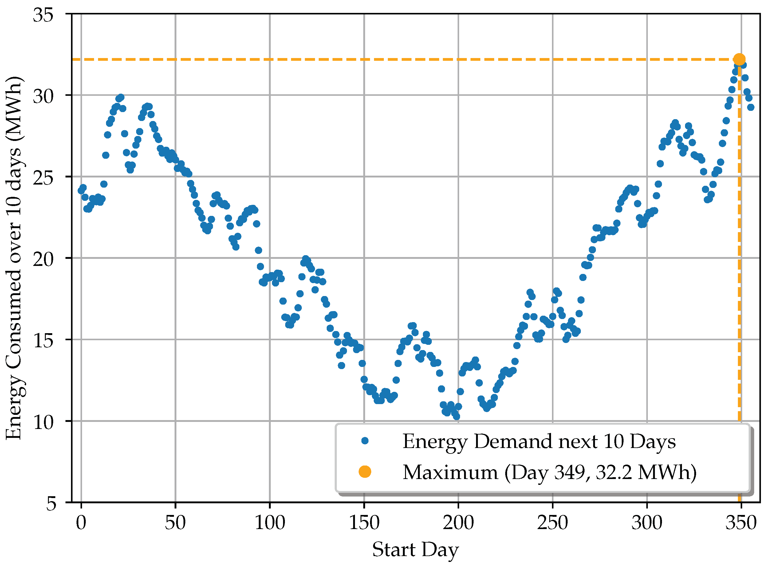
Periods of approx. 2 days, in which hardly any energy is available from wind and sun, tend to be the rule in Germany [33]. However, the claim of this paper is to assume the worst-case conditions for consideration, since sufficient energy supply must be ensured even in these conditions. Thats why a period of 10 days [34] is chosen. To determine the period with the highest energy demand occuring in the neighbourhood, 354 periods are formed. Each period starts on day X and ends after 240 $\mathrm{h}$, as shown in Figure 1. It is assumed that the thermal energy demand and the hot water energy demand in all buildings are covered by electric heat pumps and that these have a COP of 4 (for more details on this, see Section 2.5).

The maximum occurs beginning on day 349 and amounts to $32.2$ MWh of electrical energy consumed for heating, hot water supply, and direct electricity use. The resulting period to be considered thus begins on 15 December 2007 at 0:00 and ends on 24 December 2007 at 23:59:59. In Section 3.1, the energy demand during this period is analysed and presented in more detail.

2.3. Modelling Approach

The modelling approach used in this paper is based on the approach from [20], which in turn is based on a linear optimisation with variable time series resolution implemented in python using OEMOF [24,25]. Thus, investigation of thermal, electrical, hydrogen and natural gas energy flows into and out of buildings can be modelled. Self-defined notional costs are used to formulate a minimisation problem. Energy flows can be prioritised by setting these costs as desired and are therefore defined such, that no energy is drawn from the grid. However, different boundary conditions (see Section 2.5) are chosen depending on the scenario considered (see Section 2.6). The modelling approach used in this paper is based on the approach from [20], which in turn is based on a linear optimisation with variable time series resolution implemented in python using OEMOF [24,25]. Thus, investigation of thermal, electrical, hydrogen and natural gas energy flows into and out of buildings can be modelled. Self-defined notional costs are used to formulate a minimisation problem. Energy flows can be prioritised by setting these costs as desired and are therefore defined such, that no energy is drawn from the grid. However, different boundary conditions (see Section 2.5) are chosen depending on the scenario considered (see Section 2.6).

2.4. In- and Output Parameters of the Model

Figure 2 shows the input and output parameters considered in the model. The main input parameters of the model are the defined static heat and electricity demand of the building. These demands should be covered by the variable heat and electricity production from the FCEVs. Solar electricity from rooftop PV systems or electricity from the grid is not available in any of the scenarios considered. The period during which the car is coupled to the building, it can provide energy. Efficiency values of the fuel cell systems are predefined via parameters. A heat pump with a given coefficient of performance (COP) can be used for additional heat generation in the building. The model also accounts for the flexible thermal and electrical storage units. The capacity parameter of these storage units is determined via optimisation. The capacity parameters of these storage units are determined by optimization so that they are as small as possible and as large as necessary. The losses incurred and other parameters (see Section 2.5) are taken into account in the dimensioning. All variable energy flows (green boxes in Figure 2) are to be determined by the optimisation.

The result of a simulation is the determined energy flows (cf. Figure 2), for which the lowest notional costs are incurred for the given boundary conditions (see Section 2.5). The results also include the needed electrical and thermal power capacities of the FCEVs to be optimised and the capacities of the storage facilities, if available.

2.5. Optimisation Boundary Conditions

The exact boundary conditions and settings of the model are explained in more detail below. The coefficient of performance of modern heat pumps varies between average values of 3.5 to 4.5. These values are based on the requirements for obtaining a subsidy from the German Federal Office of Economics and Export Control (“Basisförderung Wohngebäude” and “Innovationsförderung” for electrical air heat pumps) [35]. Therefore, a COP of 4 is selected for the heat pump of the model building under consideration, precisely as in [20].

The degree of energy efficiency of the virtual power plant consisting out of several FCEVs is, as in [20], determined based on [21,26]. It is approximated for the simulations as follows: For every 100 kWh of chemical energy expended in the form of hydrogen, $41.87$ kWh of electrical energy and $29.77$ kWh of thermal energy are generated. This corresponds to an electrical efficiency of 41.87% and a thermal efficiency of 29.77%. However, since the power must still be fed out of the car and, if necessary, made usable (e.g., the direct current fed out must first be converted via an inverter), losses are also calculated for this. Therefore, 10% losses are taken into account for heat and 5% for electricity.

In the scenarios (cf. Section 2.6), a distinction is made between scenarios with and without storage capacities available in the buildings. If storage capacities are available, the sizes are not predefined but determined during the optimisation process. The costs are defined such, that thermal storage capacity is cheaper than electrical storage, so that the electrical storages are kept as small as possible. A round trip efficiency of 90% is taken into account for the electrical storage unit [36], and an efficiency of 92% for the thermal storage unit [21]. Storage losses that occur over time, e.g., at the heat storage, are not taken into account separately.

The specific costs are defined as such, that using energy from the FCEV is preferred over using energy from storages ($c_{EFromStorage}>c_{EFromFCEV}$). The thermal and electrical energy generated by the FCEV must be used entirely and shall not be wasted. Therefore the cost of feeding a thermal and electrical surplus sink is defined as very high. This is to prevent that, for example, only the electricity is used and the heat remains unused.

The time resolution in the optimisation is set to 15 min. As in [20], individual days are not optimised, but rather the entire period is under consideration. This is done since energy can theoretically be stored for several days and does not have to be consumed at the end of the 24 $\mathrm{h}$, as would be the case with optimisation daily. The solver used in the simulations is the “coin-or branch and cut” solver (CBC) [37].

A brief overview of the boundary conditions is given in

Table A3. Static Boundary Conditions of the Simulations.

Condition	Value
Charging Power of BEVs	0–150 kW
Coefficient of Performance of Heatpumps	4.0
Electrical Efficiency of Fuelcell Stack FCEV	0.4187
Electrical Efficiency of Electrical Storage	0.9
Electrical Transfer Losses from Car to Building	5%
Energy Density Hydrogen	33.33 kWh/kg
Electrical Energy needed per Day per BEV	5.1 kWh
Heat Transfer Losses from Car to Building	10%
Maximum Continious Electrical Power per FCEV	32 kW
Tank Volume of one FCEV	6.33 kg
Thermal Efficiency of Fuelcell Stack FCEV	0.2977
Thermal Efficiency of Thermal Storage	0.92
Time Resolution of the Simulations	15 min

in the Appendix A.

2.6. Considered Scenarios

As a derivation from the boundary conditions and the pure energy demand of the neighbourhood, the charging of battery electric vehicles, which will become increasingly relevant in the future, is also considered in the scenarios shown in

Table 3. Scenarios Considered.

Employees	BEVs Day	BEVs Night	Energy for Charging
0%	0	0	0 kWh
10%	2	9	561 kWh
25%	5	22	1377 kWh
50%	10	44	2754 kWh
75%	15	66	4131 kWh

. The number of cars to be charged and the period they are charged is defined relative to the number of employees and their working hours (cf. Table 2). For simplification, it is assumed that the vehicles are charged every weekday. In this way, weekend excursions or the charging of visitors’ cars and cars of non-employees, if applicable, are also partially taken into account in terms of energy.

The amount of energy to be charged per day for each vehicle is $5.1$ kWh. This results from the average commuting distance ($d_{cdist}$) of German employees, which bases on [38] and is calculated as follows, and the consumption of an average electric car (approx. 170 kWh km⁻¹, see [39]).

$$d_{cdist}=22.2\%\ast 7.5\mathrm{km}+30.2\%\ast 17.5\mathrm{km}+14.8\%\ast 37.5\mathrm{km}+5.1\%\ast 50\mathrm{km}=15.05\mathrm{km}$$

(2)

The following Table 3 shows all the scenarios considered:

The period overnight and over day is the same as the period used to determine the required power capabilities of the FCEVs. The BEVs can be adaptively charged with 0 kW to 150 kW during these periods. The defined amount of energy must have been charged into each vehicle at the end of the period. Each scenario is considered once with and without storage capacities in the individual residential buildings.

3. Results and Discussion

In this section, both the initial situation is examined in terms of energy and the results of the different scenarios considered are presented and discussed. Finally, the potential offered by the additional use of waste heat from the FCEVs and how much energy can be saved by this is examined.

3.1. Energy Demand Analysis

Figure 3 shows how the energy demand of the neighbourhood is composed. As can be seen in the diagram, the blue portions, i.e., the electricity demand for heating, are higher, by a factor of approx. 2 to 3 depending on the day. This is not surprising, as heating is exclusively provided by heat pumps and the period under consideration is in December. The highest energy demand occurs on 22.12. and amounts to 3543 kWh. This day will probably be decisive for optimising the required power capacities.

3.2. Capacity Requirements

Optimising the energy demand of the neighbourhood as it is with a virtual power plant consisting of a to be determined number of FCEVs (depending on the given technical framework conditions required to provide the determined power capacity) results in the needed capabilities shown in Figure 4 result. The optimisation distinguishes between two capabilities. One is determined between 19:00 and 7:00 (shown in blue and dark grey) and another between 7:00 and 19:00 (shown in orange and light grey). Thus, a statement about which capacity is required at night and during the day can be given. Furthermore, a distinction is made between a scenario without (Figure 4, left) and a scenario with storage capacities to be optimised (Figure 4, right). For determining the proportions of the virtual power plant’s thermal and electrical power capacity, the efficiency configuration of the fuel cells, comprising the virtual power plant, is decisive. The results are also given in numbers in

Table 4. Power Demand in the Neighbourhood.

Parameter	Without Storages	Including Storages
Storage EL	-	656 kWh
Overnight EL	198 kW	108 kW
Overday EL	229 kW	134 kW
Storage TH	-	699 kWh
Overnight TH	141 kW	76 kW
Overday TH	163 kW	95 kW

.

As can be seen in the graph, the required power demand is significantly lower with storage capacities in the buildings. The power demand during the day is higher than the demand during the night. This is because most residents of the neighbourhood under consideration are either sleeping or working at night. Thus, the need for hot water and electricity is comparatively lower. Without storage, the power demand is defined by the peak demand. Including storage, the lowest possible power demand is determined based on prioritisation via the notional costs. The power demand is thus rather constant. However, energy losses occur at the storage units, and, conversely, more hydrogen is needed to supply the neighbourhood, which is described in more detail in Section 3.4.

3.3. Taking Electromobility into Account

Considering the current development of electric mobility, it would be unrealistic to assume that no BEVs will be charged in a neighbourhood in the future. For this reason, the charging of BEVs is taken into account in the following scenarios. First, it is investigated how the required power capacities without storage in the residential buildings develop with an increasing number of vehicles to be charged. The results are shown in Figure 5 and numerically in

Table 5. Power demand including Electromobility, without Storage Capacities.

Par./BEVs	0	12/9	5/22	10/44	15/66
Storage EL	-	-	-	-	-
Overnight EL	198 kW	198 kW	198 kW	198 kW	198 kW
Overday EL	229 kW	229 kW	229 kW	229 kW	229 kW
Storage TH	-	-	-	-	-
Overnight TH	141 kW	141 kW	141 kW	141 kW	141 kW
Overday TH	163 kW	163 kW	163 kW	163 kW	163 kW

.

As can be seen in Figure 5, no additional power capacities are necessary. This is related to the cars being charged flexibly over 12 h, and the charging power can be reduced accordingly to 0 $\mathrm{k}$$\mathrm{W}$ at the peak loads that occur in the neighbourhood. The total amount of hydrogen consumed is higher according to the additional energy required for charging. Furthermore it is investigated, how the required power capacities develop with increasingly more BEVs to be charged if optimal storage facilities are available. The results are shown in Figure 6 and numerically in

Table 6. Power demand including Electromobility, including Storage Capacities.

Par./BEVs	0	12/9	5/22	10/44	15/66
Storage EL	656 kWh	609 kWh	630 kWh	618 kWh	618 kWh
Overnight EL	108 kW	112 kW	118 kW	130 kW	148 kW
Overday EL	134 kW	134 kW	134 kW	133 kW	126 kW
Storage TH	699 kWh	657 kWh	592 kWh	477 kWh	481 kWh
Overnight TH	76 kW	79 kW	84 kW	93 kW	106 kW
Overday TH	95 kW	95 kW	95 kW	95 kW	90 kW

.

As can be seen, the required power demand increases by 40 $\mathrm{k}$$\mathrm{W}$ of electrical power for 66 cars during nights. During the day, it decreases by 8 $\mathrm{k}$$\mathrm{W}$ of electrical power for 15 BEVs. The electrical storage necessary decreases somewhat ( $-38$ kWh for 15/66 BEVs corresponding to −6%) with an increasing number of BEVs, while the thermal storage capacity decreases significantly ( $-218$ kWh for 15/66 BEVs corresponding to −31%). This is related to the fact that a higher thermal power capacity accompanies the higher electrical power capacity at night. From the smaller storage capacity, it can be concluded that less energy from the day needs to be stored for the night. Presumably, there are power peaks during the day due to the behaviour of the residents, which is why a generally higher capacity is necessary during the day and energy is stored for the night.

As a result of the increasing number of BEVs to be charged, the power demand shifts somewhat to the night, as seen from the power demands. This trend is due to the behaviour of the residents, since more FCEVs are likely to be available at night to feed energy back into the energy grid of the neighbourhood. As in the previously examined scenarios without storage, the total amount of hydrogen consumed is higher according to the additional amounts of energy required for charging explained in more detail in the following section.

3.4. Hydrogen Consumption Analysis

The influence of an increasing number of BEVs on the required hydrogen is investigated and shown in Figure 7.

Without BEVs, an average of $205.4$ $\mathrm{k}\mathrm{g}$ of hydrogen is required daily without storage capacities. With optimal storage, $206.7$ $\mathrm{k}\mathrm{g}$ are required, which corresponds to approx. 0.6% more. The additional demand for hydrogen increases linearly with the number of BEVs and amounts to 13.5% more hydrogen for a total of 81 vehicles to be charged daily in the scenario “75% (15/66)”. The additional hydrogen demand, therefore only slightly increased (27.7 kg d⁻¹ without storage, 27.9 kg d⁻¹ with storage).

3.5. Energy Saving Potential through Waste Heat Utilisation

Since periods in which little power is available from wind and PV mainly occur in colder parts of the year, the heating demand is higher. It is a particularly relevant factor for the total amount of energy required. As already shown in Section 1, there have already been initial experiments with FCEVs feeding back energy. However, these were limited exclusively to electrical power. The additional benefit that can be derived from the waste heat of the fuel cell stack is investigated. Figure 8 shows how the total energy demand of the neighbourhood is met by shares of different energy suppliers. For example, the study is carried out on the scenario without BEVs and on the scenario “75% (15/66)”. The scenarios with storage capacities are chosen in each case, as these will probably be more realistic in the future. Since it is already known that the virtual power plant entirely covers the electrical energy demand, the outer ring of the pie charts shows wherefore the electrical energy is used. The inner-circle indicates the source of the thermal energy required for heating and domestic hot water.

As shown in the diagram on the left, just below half of the thermal energy demand can be covered by the virtual power plant consisting of FCEVs. 17% of the generated electricity is additionally used to cover the rest of the thermal need. The additional use of waste heat thus leads to a saving of $18.5$ MWh of thermal energy, respectively $4.63$ MWh of electrical energy (corresponds to approx. 14.4%).

If 81 BEVs charged daily are included in the analysis, additional heat can be used due to the higher electrical energy demand. The amount of heat supplied increases by $2.3$ MWh or 12.4%, but the heat generated by the heat pump only decreases by 800 kWh. This can be explained by the fact that the heat is not generated according to demand and has to be stored for later use-losses occur in the process. Nevertheless, this corresponds to an additional saving of about 200 kWh of electrical energy. Compared to where no waste heat would be used in this scenario, $4.83$ MWh or 13.5% of electrical energy, which would otherwise be additionally necessary for heating, is saved. The percentage of energy saved in this scenario with BEVs is correspondingly somewhat lower, as more electrical energy is required overall.

Of course, all energy savings figures refer only to the all-electric buildings in the neighbourhood. If other energy sources were used for heating, e.g., gas or wood chips, the savings would be more significant: without BEVs, 49%, with BEVs, 53% of energy can be saved for heating and domestic hot water. Likewise, it was assumed that the buildings are slightly insulated below the average building standards. In the future, it is hoped that the facilities will be insulated better and thus require less energy for heating. The percentual savings potential would then increase even further.

4. Conclusions

The simulation results have shown that FCEVs are, in principle, suitable for supplying neighbourhoods with renewable energy using green hydrogen at times when little wind and solar power is available. The additional use of waste heat increases efficiency significantly, saving up to 53% of the energy required for heating and hot water preparation.

If we take as a benchmark a Hyundai Nexo, whose fuel cell stack has a specified continuous electrical power of 32 $\mathrm{k}$$\mathrm{W}$ according to the vehicle registration certificate, then theoretically 5 FCEVs (with storage capacities in the neighbourhood) can completely cover the entire energy demand, including the electrical energy demand for charging BEVs, under all circumstances. With an increasing number of BEVs to be charged, the power demand shifts from daytime to nighttime so that even 4 FCEVs would be sufficient during the day. At five vehicles per 189 adult residents, this equates to 2.6% of adult residents required to permanently provide an FCEV. With four vehicles, it is 2.1%. In addition, this is the case for assuming the worst possible conditions for all circumstances.

However, the hydrogen required is the limiting factor with a total tank capacity of $6.33$ $\mathrm{k}\mathrm{g}$ hydrogen (at 700 bar) [40,41]. If we assume that half of the tank capacity (i.e., about $3.2$ $\mathrm{k}\mathrm{g}$ of hydrogen) is available to the vehicles every day, 75 FCEVs that need to be refuelled every day would be required instead of the five cars being theoretically sufficient in terms of their power capabilities. Consequently, it would be beneficial to supply the cars with hydrogen on a stationary basis for a technical realisation.

The accuracy of the actual achievable thermal and electrical efficiency of regenerative FCEVs is estimated in this paper based on current data. Possible dependencies of these efficiencies on external influences, such as the outside temperature, are not taken into account, since no data exist on this yet. To create a better basis for upcoming simulations, further experiments are needed. Likewise, it must be said that economic interests of the owners of the vehicles are not considered in this work. The focus is purely on the energy aspects. For an actual practical implementation of the scenarios considered, this will of course only work if the owners of the FCEVs derive an economic benefit from the provision of their vehicle. For this, the wear and tear of the equipment and the costs of the equipment required to transfer the energy from the vehicles to the corresponding local grids should be taken into account.