
Short-Term Forecasting of Energy Production for a Photovoltaic System Using a NARX-CVM Hybrid Model

 , ,
, ,  and
and 
Abstract
:1. Introduction
2. Mathematical Models
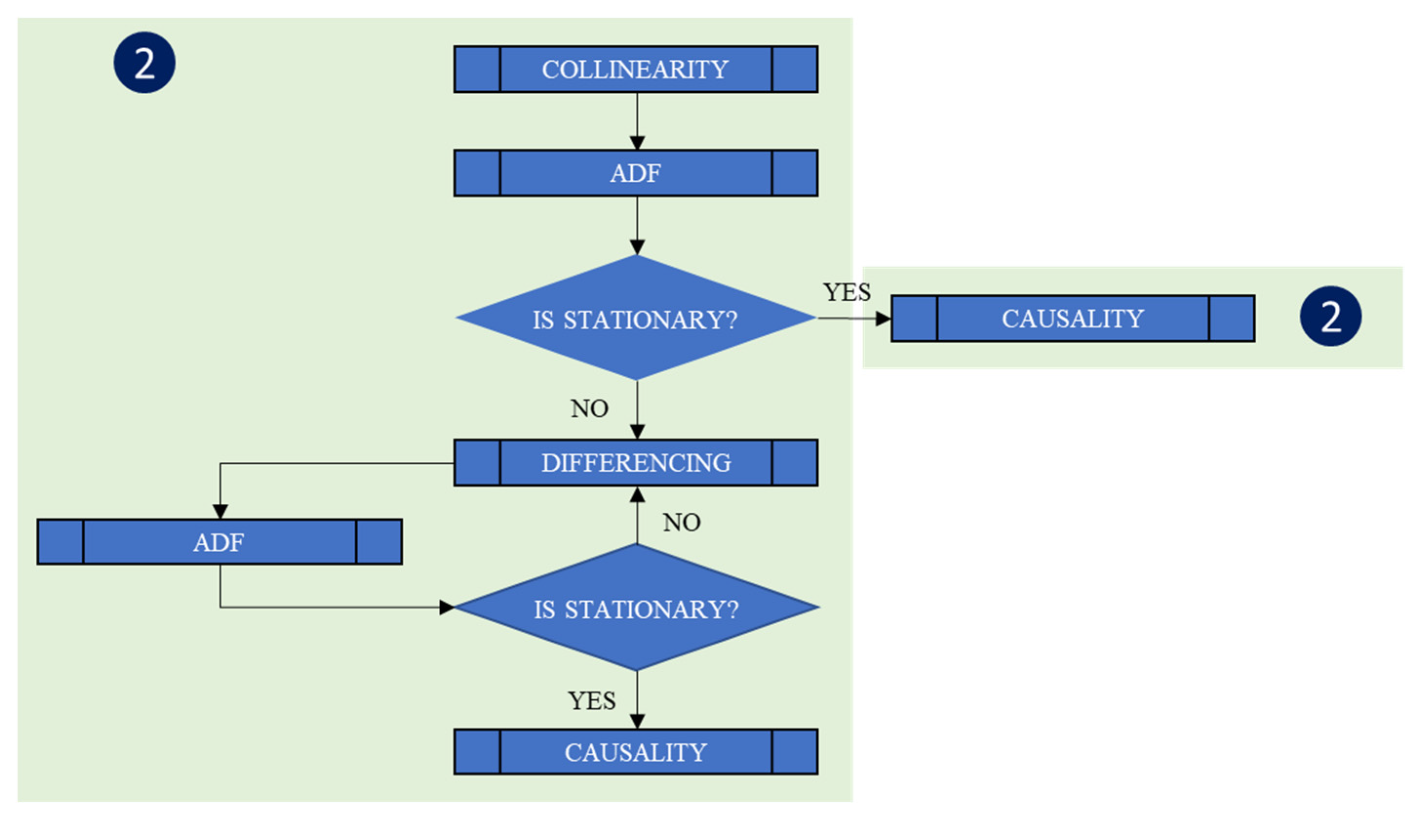
2.1. Collinearity Test
2.2. Augmented Dickey–Fuller Test
2.3. Engle–Granger Causality Test
- does not Granger cause ;
- Granger causes .
- <0.01 Granger causes at the 1%;
- >0.01 does not Granger cause at the 1%.
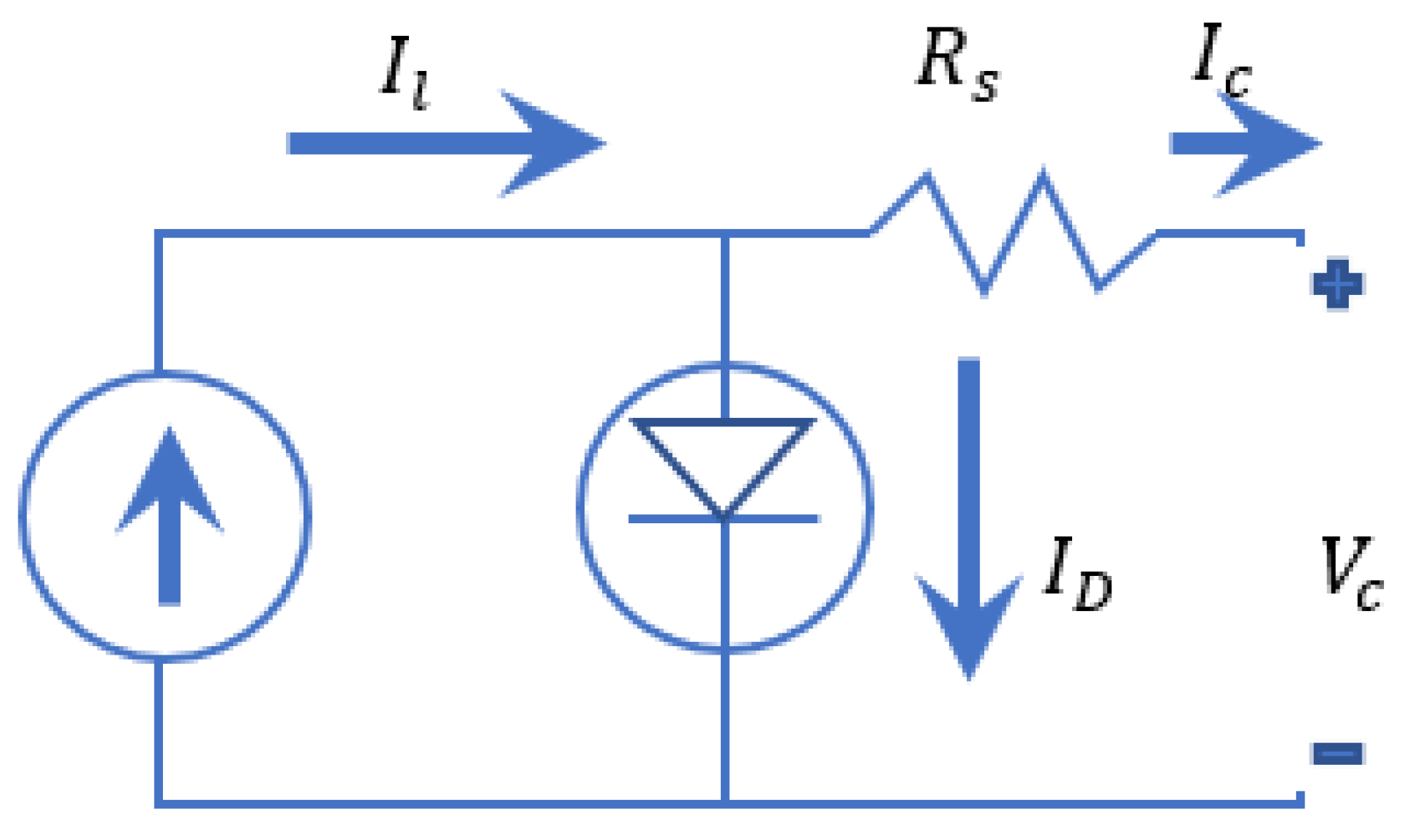
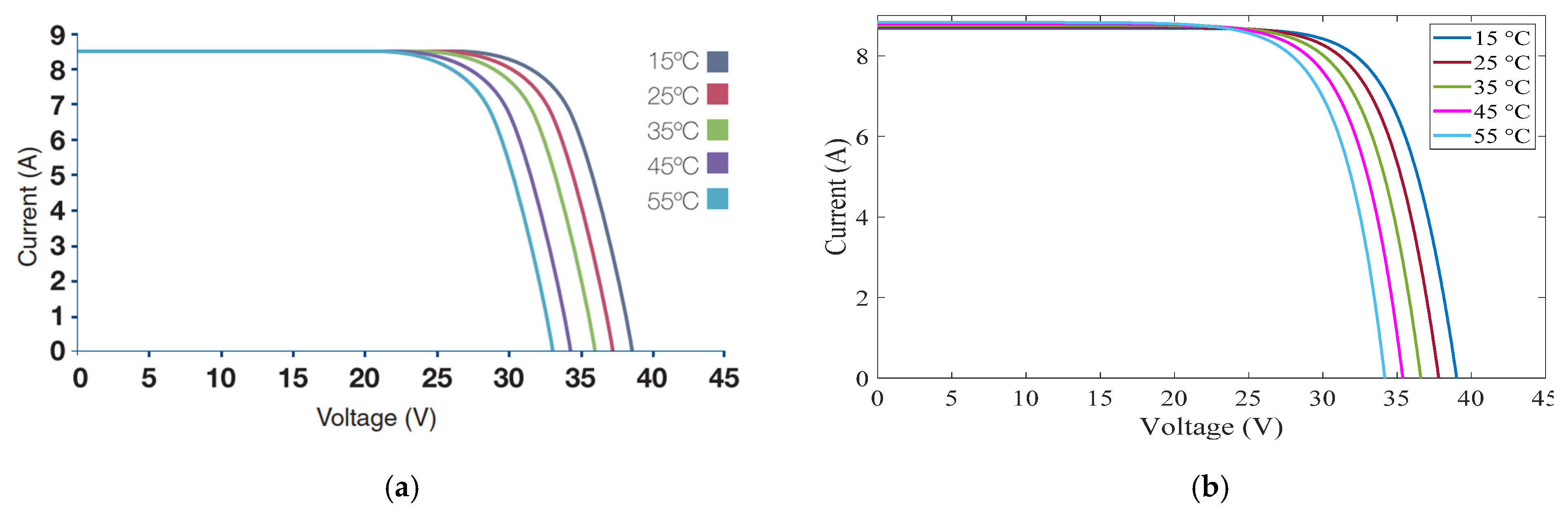
2.4. Simplified Single Diode Model
2.5. Solar Radiation under Clear Sky Conditions
2.6. Calculation of the Turbidity Factor
- At least one day of each month is completely clear and corresponds to the day that records the maximum SR measured for that month.
- For each month of the year, the maximum extraterrestrial SR value was calculated to each maximum extraterrestrial SR value corresponding to a value of .
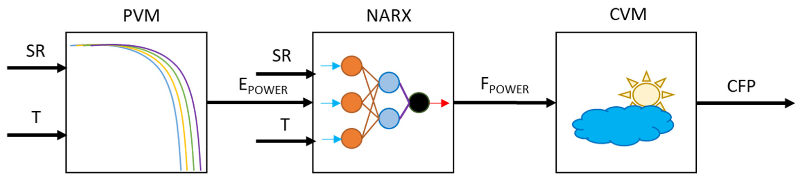
3. Methodology for Building the NARX-CVM Hybrid Model
3.1. Step 1: Databases (VARIABLES)
3.2. Step 2: Selecting the Input Variables (INPUTS)
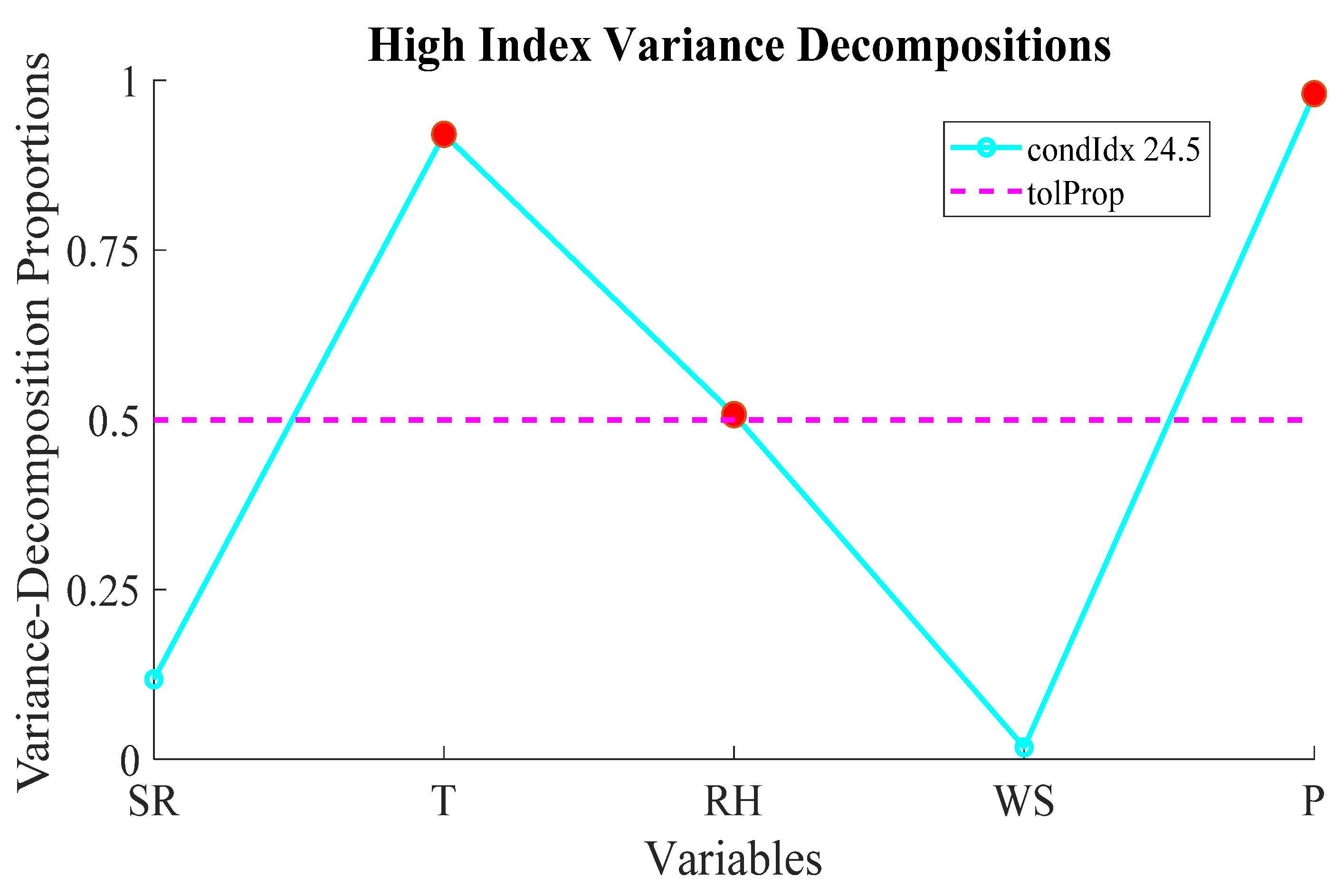
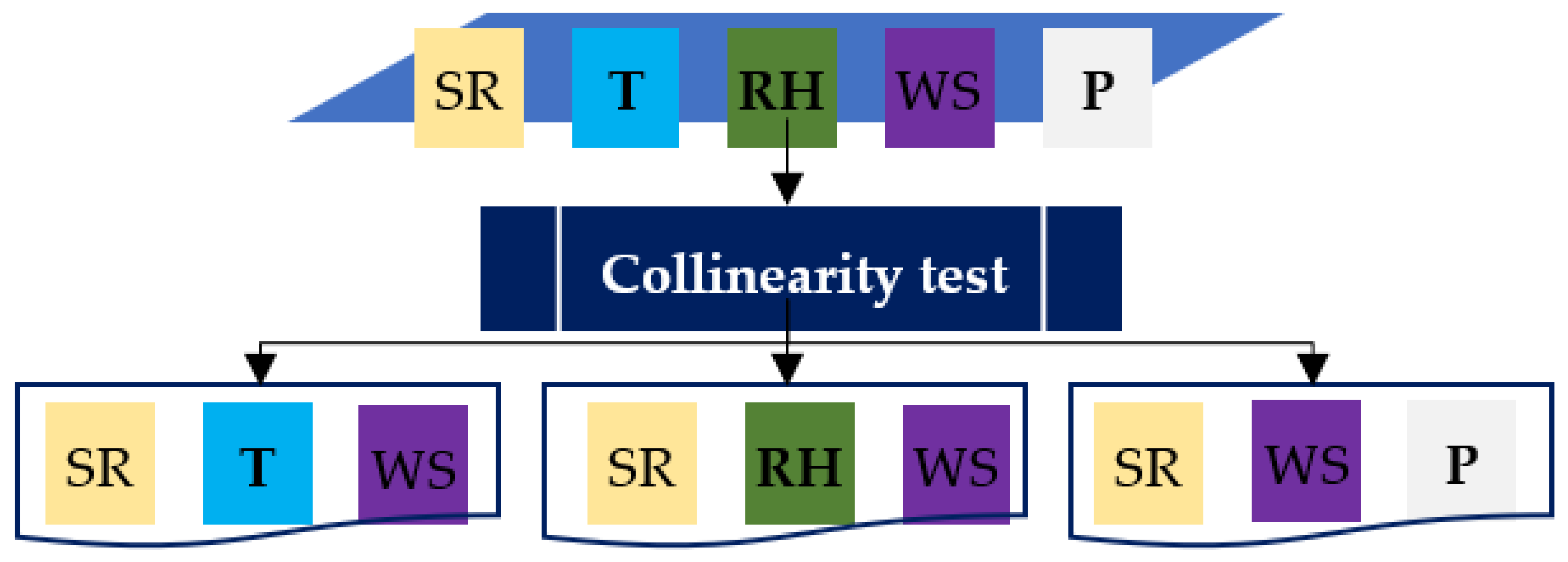
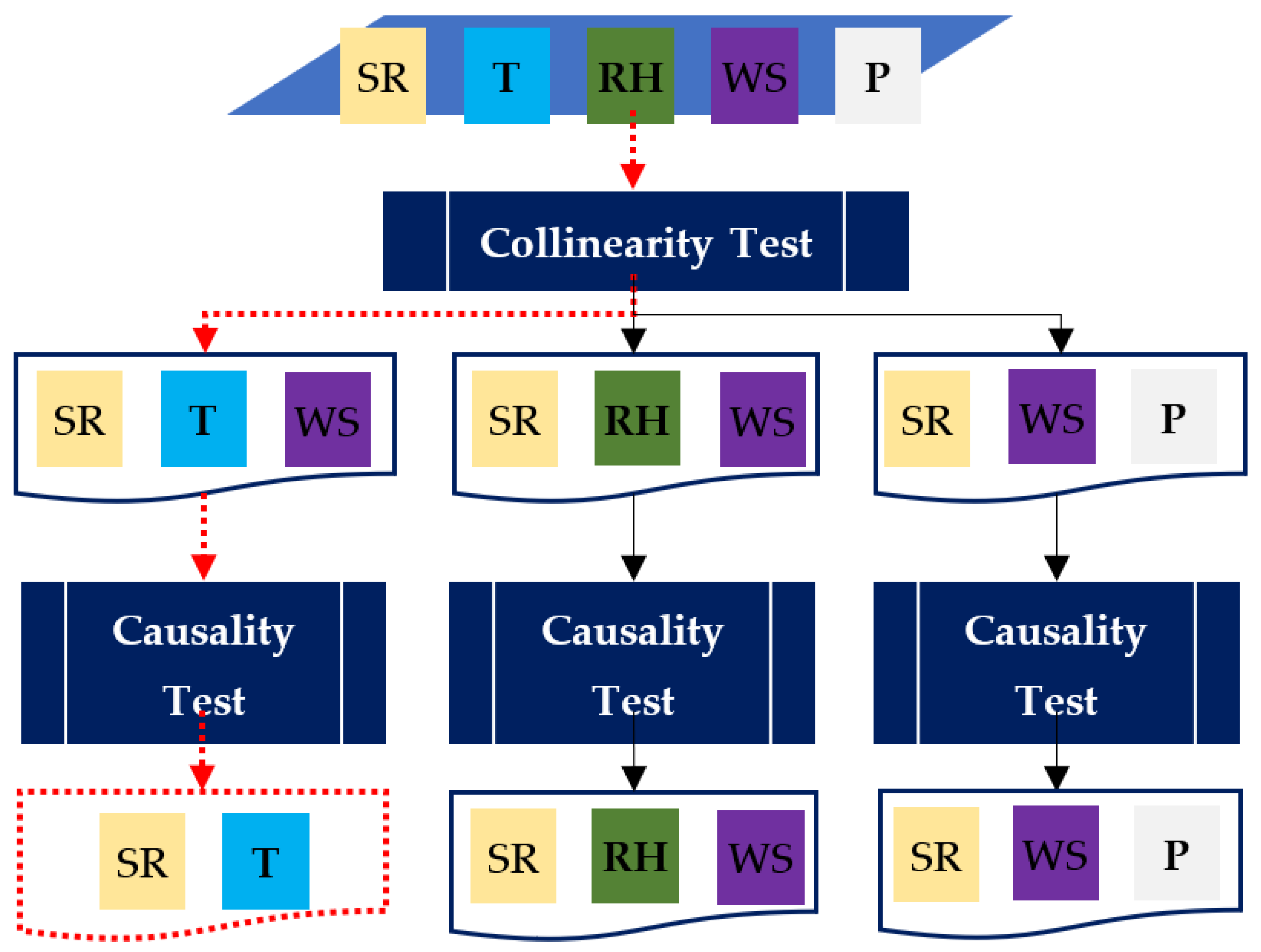
3.2.1. Collinearity Test
3.2.2. Augmented Dickey–Fuller Test (ADF)
3.2.3. Engle–Granger Causality Test Results
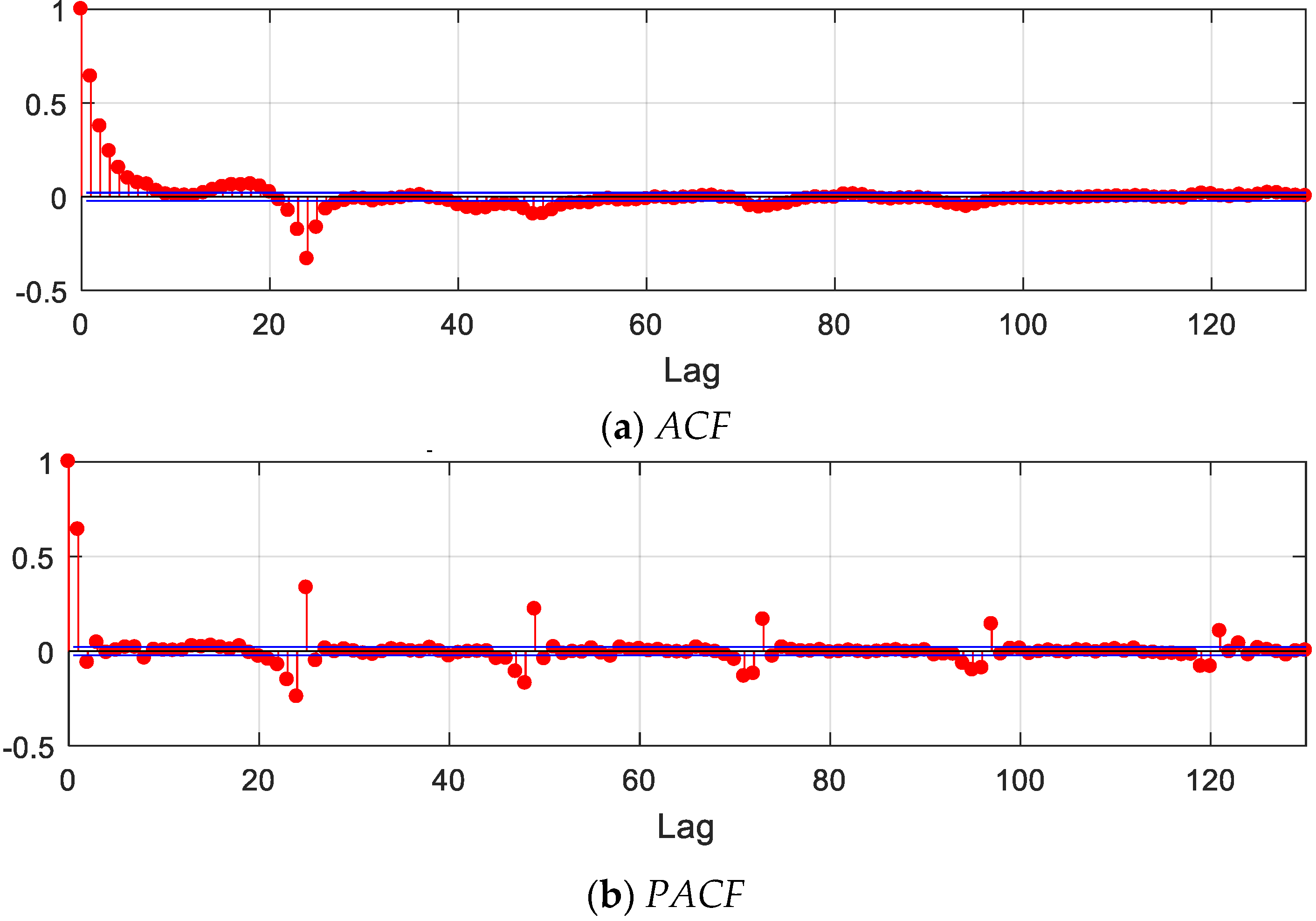
3.3. Step 3: Lags for the NARX Model (LAGS)
3.4. Step 4: Modeling Photovoltaic Systems
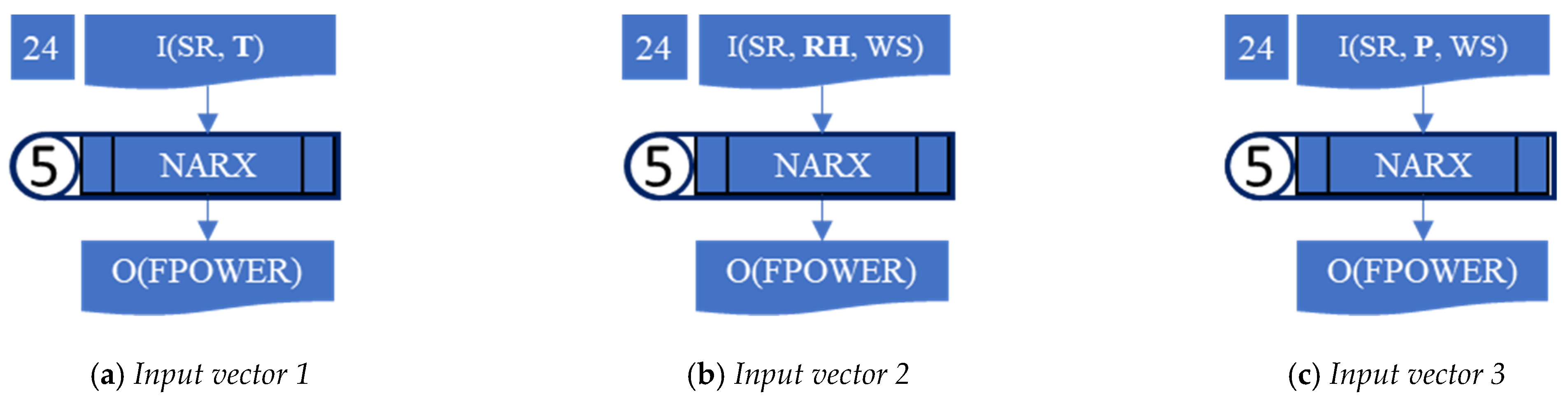
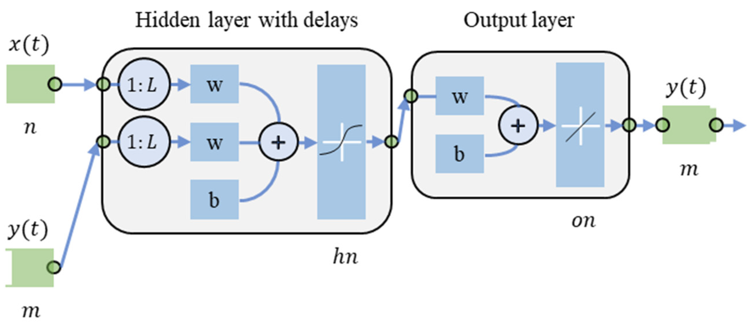
3.5. Step 5: Multivariable Forecasting Model (NARX)
3.6. Step 6: Output Data Depuration of the Forecasting Model (CVM)
4. Performance Tests
5. Results and Discussion
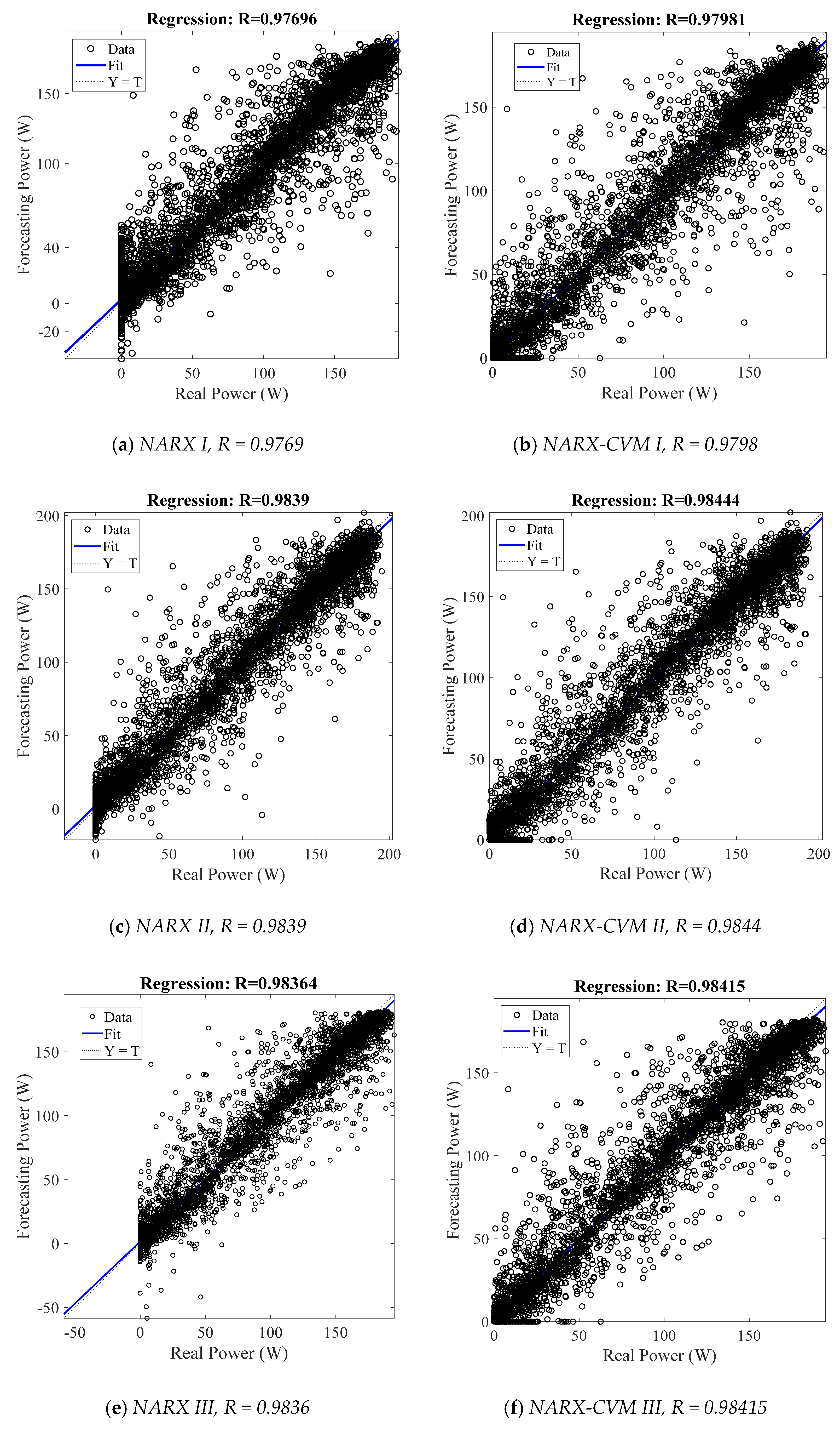
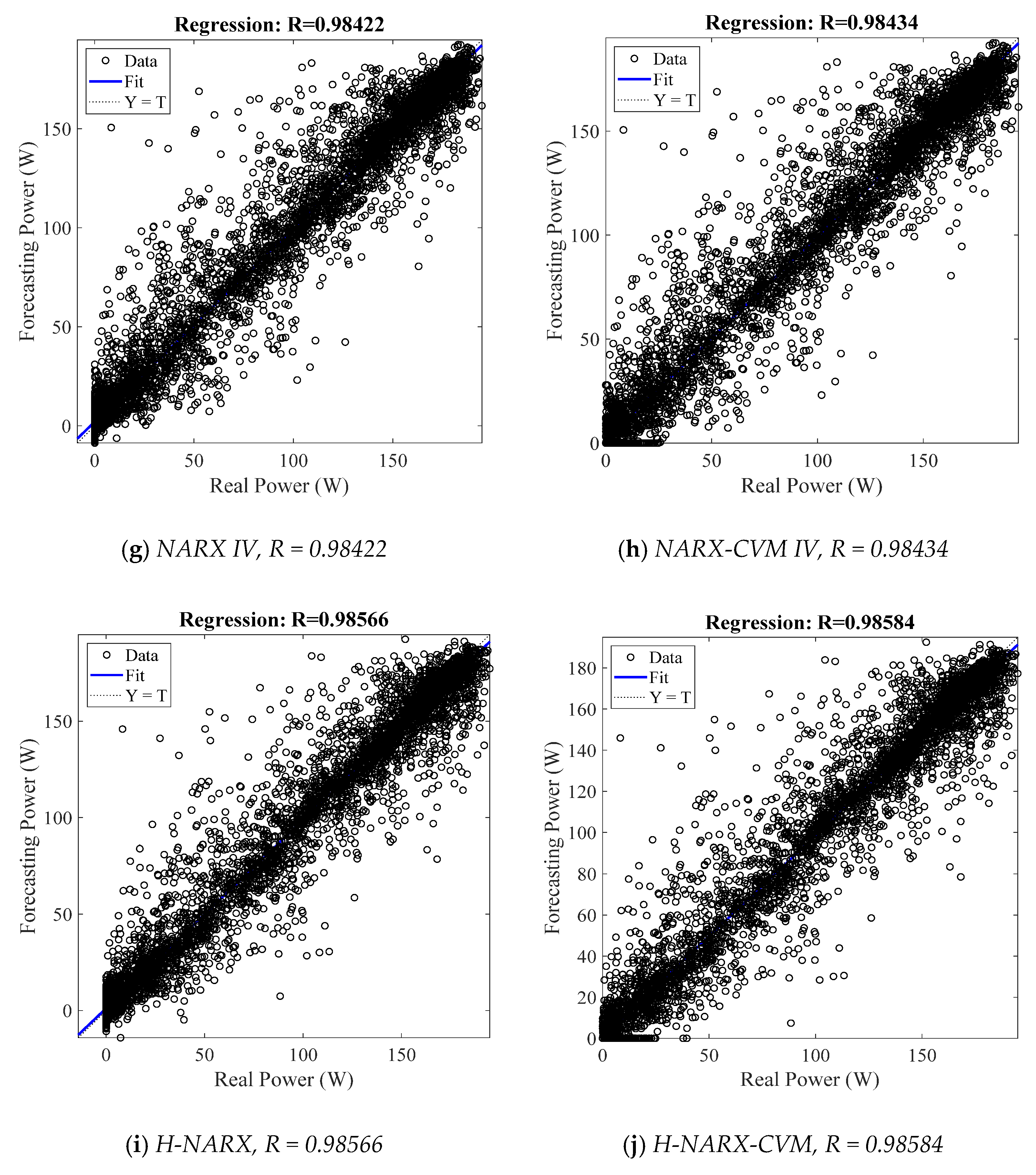
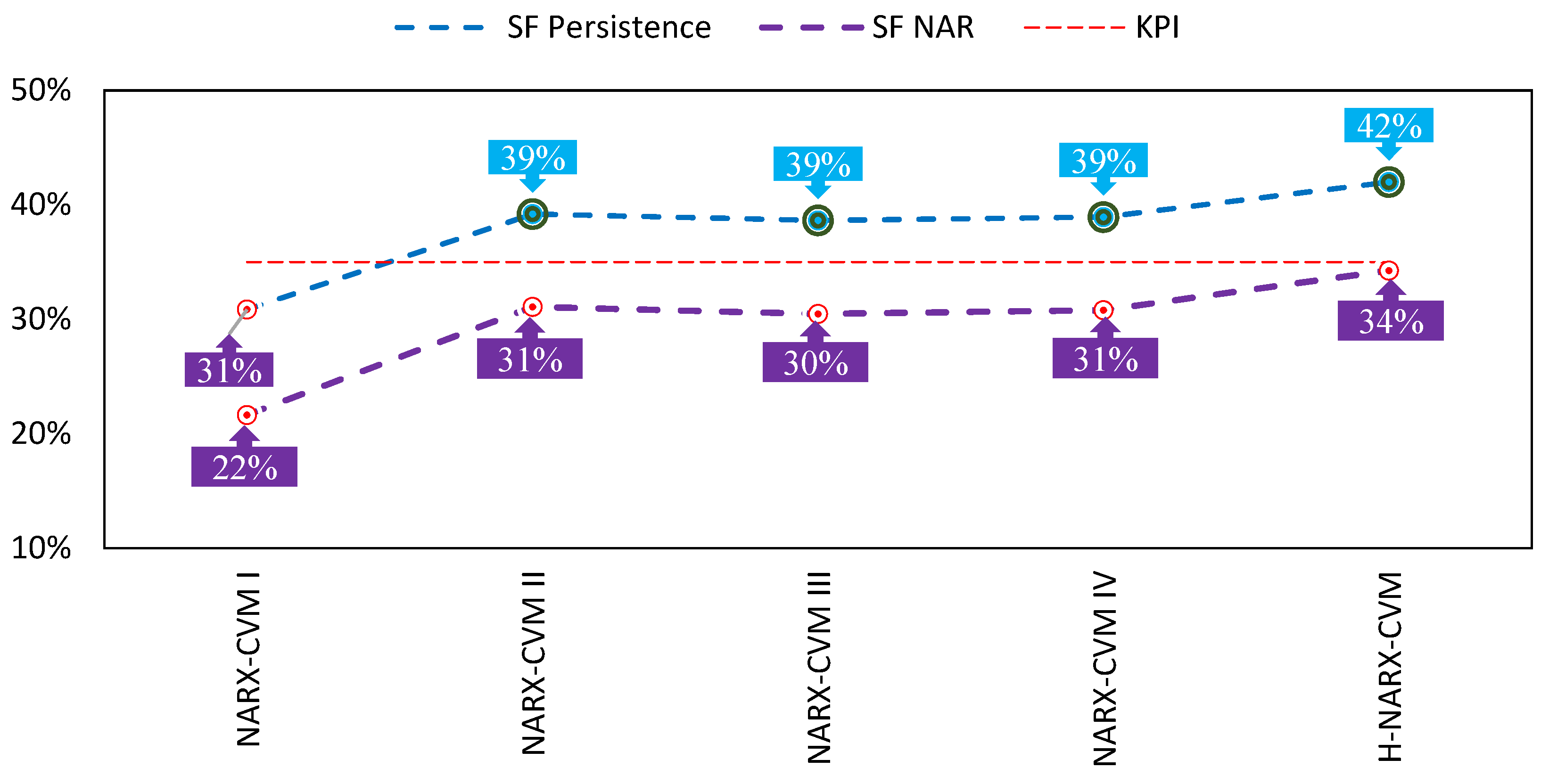
5.1. Comparison between Models with and without CVM
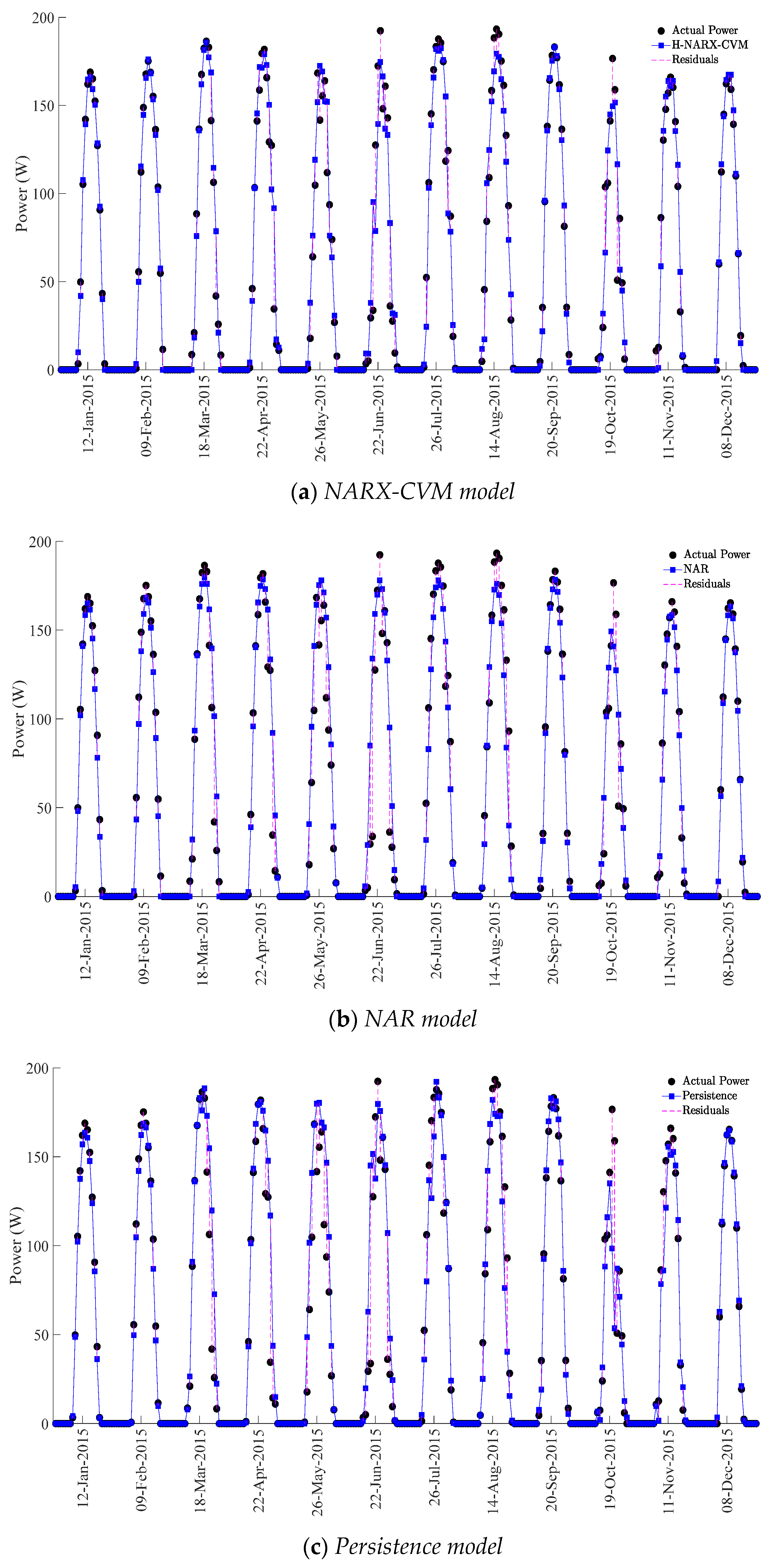
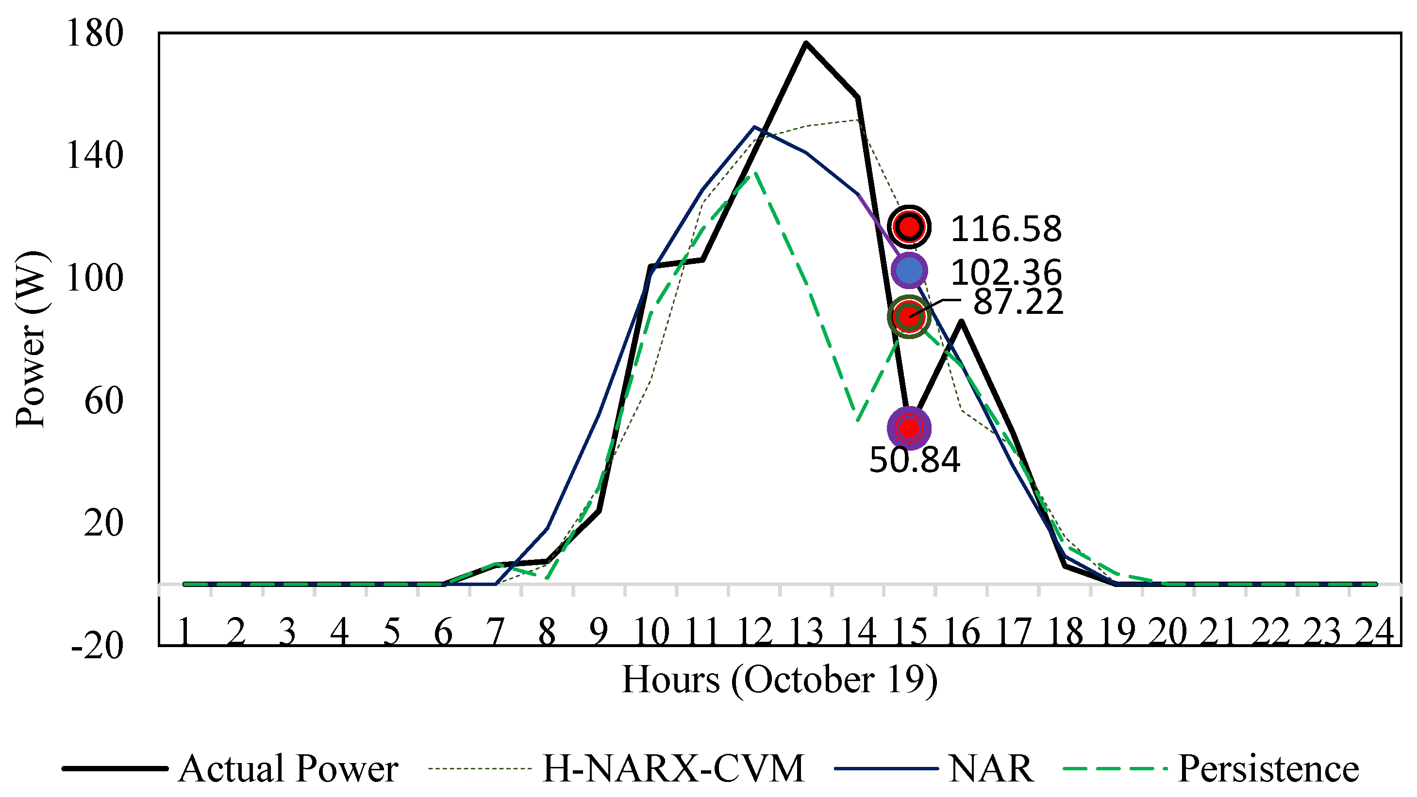
5.2. Comparison of the H-NARX-CVM Model against Other Models
- (1)
- The blind prediction of the power obtained using the proposed methodology;
- (2)
- The blind prediction using the NAR model;
- (3)
- The prediction using the persistence model.
6. Conclusions
Author Contributions
Funding
Institutional Review Board Statement
Informed Consent Statement
Acknowledgments
Conflicts of Interest
Abbreviations
| ANN | Artificial neural network |
| ADF | Augmented Dickey–Fuller test |
| ACF | Autocorrelation function |
| CFP | Corrected forecasting power |
| CVM | Corrective vector multiplier |
| EP | Electric power |
| H-NARX-CVM | Hibrid NARX model |
| KPI | Key performance index |
| NOCT | Nominal operating cell temperature |
| NAR | Nonlinear autoregressive |
| NARX | Nonlinear autoregressive with exogenous inputs |
| PACF | Partial autocorrelation function |
| PGM | Photovoltaic generating model |
| PVG | Photovoltaic generator |
| PVM | Photovoltaic module |
| P | Pressure |
| RH | Relative humidity |
| SR | Solar radiation |
| T | Temperature |
| WS | Wind speed |
References
- Cao, J.; Lin, X. Study of Hourly and Daily Solar Irradiation Forecast Using Diagonal Recurrent Wavelet Neural Networks. Energy Convers. Manag. 2008, 49, 1396–1406. [Google Scholar] [CrossRef]
- Hocaoǧlu, F.O.; Gerek, Ö.N.; Kurban, M. Hourly Solar Radiation Forecasting Using Optimal Coefficient 2-D Linear Filters and Feed-Forward Neural Networks. Sol. Energy 2008, 82, 714–726. [Google Scholar] [CrossRef]
- Akarslan, E.; Hocaoglu, F.O. A Novel Adaptive Approach for Hourly Solar Radiation Forecasting. Renew. Energy 2016, 87, 628–633. [Google Scholar] [CrossRef]
- Boland, J.; David, M.; Lauret, P. Short Term Solar Radiation Forecasting: Island versus Continental Sites. Energy 2016, 113, 186–192. [Google Scholar] [CrossRef]
- Jiménez-Pérez, P.F.; Mora-López, L. Modeling and Forecasting Hourly Global Solar Radiation Using Clustering and Classification Techniques. Sol. Energy 2016, 135, 682–691. [Google Scholar] [CrossRef]
- Martín, L.; Zarzalejo, L.F.; Polo, J.; Navarro, A.; Marchante, R.; Cony, M. Prediction of Global Solar Irradiance Based on Time Series Analysis: Application to Solar Thermal Power Plants Energy Production Planning. Sol. Energy 2010, 84, 1772–1781. [Google Scholar] [CrossRef]
- Monjoly, S.; André, M.; Calif, R.; Soubdhan, T. Hourly Forecasting of Global Solar Radiation Based on Multiscale Decomposition Methods: A Hybrid Approach. Energy 2017, 119, 288–298. [Google Scholar] [CrossRef]
- Azimi, R.; Ghayekhloo, M.; Ghofrani, M. A Hybrid Method Based on a New Clustering Technique and Multilayer Perceptron Neural Networks for Hourly Solar Radiation Forecasting. Energy Convers. Manag. 2016, 118, 331–344. [Google Scholar] [CrossRef]
- Benmouiza, K.; Cheknane, A. Forecasting Hourly Global Solar Radiation Using Hybrid K-Means and Nonlinear Autoregressive Neural Network Models. Energy Convers. Manag. 2013, 75, 561–569. [Google Scholar] [CrossRef]
- Chen, C.-R.; Kartini, U. K-Nearest Neighbor Neural Network Models for Very Short-Term Global Solar Irradiance Forecasting Based on Meteorological Data. Energies 2017, 10, 186. [Google Scholar] [CrossRef] [Green Version]
- Voyant, C.; Muselli, M.; Paoli, C.; Nivet, M.L. Hybrid Methodology for Hourly Global Radiation Forecasting in Mediterranean Area. Renew. Energy 2013, 53, 1–11. [Google Scholar] [CrossRef] [Green Version]
- Ji, W.; Chee, K.C. Prediction of Hourly Solar Radiation Using a Novel Hybrid Model of ARMA and TDNN. Sol. Energy 2011, 85, 808–817. [Google Scholar] [CrossRef]
- Renno, C.; Petito, F.; Gatto, A. ANN Model for Predicting the Direct Normal Irradiance and the Global Radiation for a Solar Application to a Residential Building. J. Clean. Prod. 2016, 135, 1298–1316. [Google Scholar] [CrossRef]
- Kaplanis, S.; Kaplani, E. Stochastic Prediction of Hourly Global Solar Radiation for Patra, Greece. Appl. Energy 2010, 87, 3748–3758. [Google Scholar] [CrossRef]
- Sfetsos, A.; Coonick, A.H. Univariate and Multivariate Forecasting of Hourly Solar Radiation with Artificial Intelligence Techniques. Sol. Energy 2000, 68, 169–178. [Google Scholar] [CrossRef]
- Zhu, T.; Guo, Y.; Li, Z.; Wang, C. Solar Radiation Prediction Based on Convolution Neural Network and Long Short-Term Memory. Energies 2021, 14, 8498. [Google Scholar] [CrossRef]
- Zhu, T.; Li, Y.; Li, Z.; Guo, Y.; Ni, C. Inter-Hour Forecast of Solar Radiation Based on Long Short-Term Memory with Attention Mechanism and Genetic Algorithm. Energies 2022, 15, 1062. [Google Scholar] [CrossRef]
- Hedar, A.R.; Almaraashi, M.; Abdel-Hakim, A.E.; Abdulrahim, M. Hybrid Machine Learning for Solar Radiation Prediction in Reduced Feature Spaces. Energies 2021, 14, 7970. [Google Scholar] [CrossRef]
- Jo, S.C.; Jin, Y.G.; Yoon, Y.T.; Kim, H.C. Methods for Integrating Extraterrestrial Radiation into Neural Network Models for Day-Ahead Pv Generation Forecasting. Energies 2021, 14, 2601. [Google Scholar] [CrossRef]
- Hocaoglu, F.O.; Serttas, F. A Novel Hybrid (Mycielski-Markov) Model for Hourly Solar Radiation Forecasting. Renew. Energy 2017, 108, 635–643. [Google Scholar] [CrossRef]
- Wang, F.; Mi, Z.; Su, S.; Zhao, H. Short-Term Solar Irradiance Forecasting Model Based on Artificial Neural Network Using Statistical Feature Parameters. Energies 2012, 5, 1355–1370. [Google Scholar] [CrossRef] [Green Version]
- Yadav, A.K.; Malik, H.; Chandel, S.S. Selection of Most Relevant Input Parameters Using WEKA for Artificial Neural Network Based Solar Radiation Prediction Models. Renew. Sustain. Energy Rev. 2014, 31, 509–519. [Google Scholar] [CrossRef]
- Kaushika, N.D.; Tomar, R.K.; Kaushik, S.C. Artificial Neural Network Model Based on Interrelationship of Direct, Diffuse and Global Solar Radiations. Sol. Energy 2014, 103, 327–342. [Google Scholar] [CrossRef]
- Cadenas, E.; Rivera, W.; Campos-Amezcua, R.; Cadenas, R. Wind Speed Forecasting Using the NARX Model, Case: La Mata, Oaxaca, México. Neural Comput. Appl. 2015, 27, 2417–2428. [Google Scholar] [CrossRef]
- Ahmad, A.; Anderson, T.N.; Lie, T.T. Hourly Global Solar Irradiation Forecasting for New Zealand. Sol. Energy 2015, 122, 1398–1408. [Google Scholar] [CrossRef] [Green Version]
- Alzahrani, A.; Kimball, J.W.; Dagli, C. Predicting Solar Irradiance Using Time Series Neural Networks. Procedia Comput. Sci. 2014, 36, 623–628. [Google Scholar] [CrossRef] [Green Version]
- Rangel, E.; Cadenas, E.; Campos-Amezcua, R.; Tena, J.L. Enhanced Prediction of Solar Radiation Using NARX Models with Corrected Input Vectors. Energies 2020, 13, 2576. [Google Scholar] [CrossRef]
- Belsley, D.; Kuh, E.; Welsch, R. Regression Diagnostics—Identifying Influential Data and Sources of Collinearity; John Wiley & Sons, Inc.: Hoboken, NJ, USA, 1980. [Google Scholar]
- Gujarati, N.D.; Porter, D.C. Basic Econometrics, 5th ed.; Anne, E.H., Ed.; Douglas Reiner: New York, NY, USA, 2009. [Google Scholar]
- Makridakis, S.G.; Wheelwright, S.C.; Hyndman, R.J. Forecasting Methods and Applications, 3rd ed.; Wiley: Hoboken, NJ, USA, 1997. [Google Scholar]
- Montgomery, D.C.; Jennings, C.L.; Kulahci, M. Introduction to Time Series Analysis and Forecasting, 2nd ed.; Wiley: Hoboken, NJ, USA, 2015. [Google Scholar]
- Hocaoglu, F.O.; Karanfil, F. A Time Series-Based Approach for Renewable Energy Modeling. Renew. Sustain. Energy Rev. 2013, 28, 204–214. [Google Scholar] [CrossRef]
- Salas, V.Ã.; Olías, E.; Barrado, A.; Lázaro, A. Review of the Maximum Power Point Tracking Algorithms for Stand-Alone Photovoltaic Systems. Sol. Energy Mater. Sol. Cells 2006, 90, 1555–1578. [Google Scholar] [CrossRef]
- Skoplaki, E.; Palyvos, J.A. On the Temperature Dependence of Photovoltaic Module Electrical Performance: A Review of Efficiency/Power Correlations. Sol. Energy 2009, 83, 614–624. [Google Scholar] [CrossRef]
- Farivar, G.; Asaei, B. Photovoltaic Module Single Diode Model Parameters Extraction Based on Manufacturer Datasheet Parameters. In Proceedings of the PECon2010—2010 IEEE International Conference on Power and Energy, Kuala Lumpur, Malaysia, 29 November–1 December 2010; pp. 929–934. [Google Scholar] [CrossRef]
- Castañer, L.; Silvestre, S. Modelling Photovoltaic Sistems Using PSpice; John Wiley & Sons, Ltd.: Barcelona, Spain, 2002. [Google Scholar]
- Tiwari, G.N.; Tiwari, A.; Shyam. Handbook of Solar Energy, 1st ed.; Springer: Singapore, 2016. [Google Scholar]
- Behar, O.; Khellaf, A.; Mohammedi, K. Comparison of Solar Radiation Models and Their Validation under Algerian Climate—The Case of Direct Irradiance. Energy Convers. Manag. 2015, 98, 236–251. [Google Scholar] [CrossRef]
- IER-UNAM ELSOMET-IER. Available online: http://esolmet.ier.unam.mx/index.html (accessed on 31 December 2016).
- MONOCRYSTALLINE MODULE ISF-250 BLACK. Available online: http://www.solarypsi.org/repository/documents/445_Second/250-black_usa_.pdf (accessed on 1 August 2021).
- Aguiar, L.M.; Pereira, B.; Lauret, P.; Díaz, F.; David, M. Combining Solar Irradiance Measurements, Satellite-Derived Data and a Numerical Weather Prediction Model to Improve Intra-Day Solar Forecasting. Renew. Energy 2016, 97, 599–610. [Google Scholar] [CrossRef] [Green Version]
- Aryaputera, A.W.; Yang, D.; Zhao, L.; Walsh, W.M. Very Short-Term Irradiance Forecasting at Unobserved Locations Using Spatio-Temporal Kriging. Sol. Energy 2015, 122, 1266–1278. [Google Scholar] [CrossRef]
- Chu, Y.; Pedro, H.T.C.; Coimbra, C.F.M. Hybrid Intra-Hour DNI Forecasts with Sky Image Processing Enhanced by Stochastic Learning. Sol. Energy 2013, 98, 592–603. [Google Scholar] [CrossRef]
- Huang, R.; Huang, T.; Gadh, R.; Li, N. Solar Generation Prediction Using the ARMA Model in a Laboratory-Level Micro-Grid. In Proceedings of the 2012 IEEE 3rd International Conference on Smart Grid Communications, SmartGridComm, Tainan, Taiwan, 5–8 November 2012; IEEE: Piscataway, NJ, USA, 2012; pp. 528–533. [Google Scholar] [CrossRef]
- Voyant, C.; Muselli, M.; Paoli, C.; Nivet, M.-L. Optimization of an Artificial Neural Network Dedicated to the Multivariate Forecasting of Daily Global Radiation. Energy 2011, 36, 348–359. [Google Scholar] [CrossRef] [Green Version]
- Benmouiza, K.; Cheknane, A. Small-Scale Solar Radiation Forecasting Using ARMA and Nonlinear Autoregressive Neural Network Models. Theor. Appl. Climatol. 2016, 124, 945–958. [Google Scholar] [CrossRef]
- García Tena, J.L.; Cadenas Calderón, E.; Rangel Heras, E.; Morales Ontiveros, C. Generating Electrical Demand Time Series Applying SRA Technique to Complement NAR and SARIMA Models. Energy Effic. 2019, 12, 1751–1769. [Google Scholar] [CrossRef]

| Probe | Sensor | Range | Accuracy |
|---|---|---|---|
| CS500 Temperature probe | platinum resistance, DIM43760B | −40.0 °C to +60.0 °C | ±0.5 °C |
| CS500 Relative humidity probe | Vaisala INTERCAP | 0 to 100% | ±3% |
| R.M. Young wind sentry anemometer | Cups Wheel Assembly | 0.0 to 50.0 m/s | ±0.5 m/s |
| PTB110 Barometer | Vaisala BAROCAP | 500.0–1100.0 hPa | ±0.3 hPa |
| WXT510 Weather transmitter | Ultrasonic Signal BAROCAP THERMOCAP Sensor HUMICAP Sensor | 0 to 60 m/s 600 to 1100 hPa −52.0 °C to 60.0 °C 0 to 100% RH | 3% ±0.5 hPa ±0.3 °C ±3% RH |
| Variable | Durbin–Watson Statistic | Critical Value | T–Statistic | p–Valor |
|---|---|---|---|---|
| SR | 2.00 | −1.94 | −1.31 | 0.18 |
| T | 2.00 | −1.94 | −0.40 | 0.54 |
| RH | 2.00 | −1.94 | −1.46 | 0.13 |
| WS | 1.99 | −1.94 | −1.71 | 0.08 |
| P | 1.99 | −1.94 | −0.02 | 0.67 |
| |
| Variable | Probability |
| T | 0.00 |
| WS | 0.12 |
| |
| Variable | Probability |
| RH | 0.00 |
| WS | 0.00 |
| |
| Variable | Probability |
| P | 0.00 |
| WS | 0.00 |
| Parameter | Characteristics |
|---|---|
| Solar cell | Monocrystalline silicon–156 mm × 156 mm (6 inches) |
| Number of cells | 60 cells (6 × 10) |
| Dimensions | 1667 × 994 × 45 mm (65.63 × 39.13 × 1.77 in) |
| Weight | 19 kg (41.89 pounds) |
| Glass | High transmittance, patterned, tempered, 3.2 mm (EN-12150) |
| Frame | Anodized aluminium, grounding drills |
| Maximum mechanical load | 5400 Pa (112.78 psf) (Snow load) |
| Junction box | IP 65 with three bypass diodes |
| Cables, plug | Solar cable 1 m (39.37 in), four mm2 (12 AWG). MC4 or LC4 |
| Parameter | Characteristics |
|---|---|
| Rated power (Pmax) | 250 W |
| Open-circuit voltage (Voc) | 37.8 V |
| Short-circuit current (Isc) | 8.75 A |
| Maximum power point voltage (Vmax) | 30.6 V |
| Maximum power point current (Imax) | 8.17 A |
| Efficiency | 15.1% |
| Power tolerance (% Pmax) | 0/+3% |
| Variable | Estimated | Actual | Error |
|---|---|---|---|
| 248.1 | 250.0 | 0.75% | |
| 37.5 | 37.8 | 0.83% | |
| 30.8 | 30.6 | −0.78% | |
| 8.8 | 8.8 | −0.12% | |
| 8.1 | 8.2 | 1.52% |
| Models | Lags | Input | Output | Tests | ||
|---|---|---|---|---|---|---|
| NARX I | 24 | SR, T, RH, WS, P | FPOWER | 10 | 1 | All variables |
| NARX II | 24 | SR, T, WS | FPOWER | 10 | 1 | Collinearity and causality |
| NARX III | 24 | SR, RH, WS | FPOWER | 10 | 1 | Collinearity and causality |
| NARX IV | 24 | SR, WS, P | FPOWER | 10 | 1 | Collinearity and causality |
| H-NARX | 24 | SR, T | FPOWER | 10 | 1 | Collinearity and causality |
| Model | Lag | Input | Output | MBE (W) | MSE (W2) | RMSE (W) | R2 |
|---|---|---|---|---|---|---|---|
| NARX I | 24 | SR, T, RH, WS, P | FPower | 0.45 | 210.30 | 14.50 | 0.95 |
| NARX II | 24 | SR, T, WS | FPower | 0.70 | 147.83 | 12.16 | 0.97 |
| NARX III | 24 | SR, RH, WS | FPower | −0.27 | 149.81 | 12.24 | 0.97 |
| NARX IV | 24 | SR, WS, P | FPower | 0.72 | 145.15 | 12.05 | 0.97 |
| H-NARX | 24 | SR, T | FPower | −0.18 | 131.42 | 11.46 | 0.97 |
| Model | Lag | Input | Output | cMBE (W) | cMSE (W2) | cRMSE (W) | cR2 |
|---|---|---|---|---|---|---|---|
| NARX-CVM I | 24 | SR, T, RH, WS, P | CPower | −0.45 | 184.80 | 13.59 | 0.96 |
| NARX-CVM II | 24 | SR, T, WS | CPower | −0.01 | 142.78 | 11.95 | 0.97 |
| NARX-CVM III | 24 | SR, RH, WS | CPower | −0.57 | 145.41 | 12.06 | 0.97 |
| NARX-CVM IV | 24 | SR, WS, P | CPower | 0.40 | 143.96 | 12.00 | 0.97 |
| H-NARX-CVM | 24 | SR, T | CPower | −0.41 | 130.07 | 11.40 | 0.97 |
| Model | RMSE (W) | cRMSE (W) | Improvement |
|---|---|---|---|
| NARX I vs. NARX-CVM I | 14.50 | 13.59 | 6.7% |
| NARX II vs. NARX-CVM II | 12.16 | 11.95 | 1.8% |
| NARX III vs. NARX-CVM III | 12.24 | 12.06 | 1.5% |
| NARX IV vs. NARX-CVM IV | 12.05 | 12.00 | 0.4% |
| H-NARX vs. H-NARX-CVM | 11.46 | 11.40 | 0.5% |
| Models | Performance Tests | |||
|---|---|---|---|---|
| MBE | MSE | RMSE | R2 | |
| H-NARX-CVM | −0.41 | 130.07 | 11.40 | 0.97 |
| NAR | −1.12 | 300.57 | 17.34 | 0.94 |
| Persistence | 0.00 | 386.12 | 19.65 | 0.92 |
| Models | Performance Tests | |||
|---|---|---|---|---|
| MBE | MSE | RMSE | R2 | |
| H-NARX-CVM | 0.08 | 142.59 | 11.94 | 0.97 |
| NAR | 0.56 | 220.54 | 14.85 | 0.95 |
| Persistence | 1.48 | 330.01 | 18.17 | 0.93 |
| Models | Performance Tests | |||
|---|---|---|---|---|
| MBE | MSE | RMSE | R2 | |
| H-NARX-CVM | −0.29 | 329.36 | 18.15 | 0.90 |
| NAR | 1.12 | 291.60 | 17.08 | 0.91 |
| Persistence | −6.89 | 803.77 | 28.35 | 0.78 |
Publisher’s Note: MDPI stays neutral with regard to jurisdictional claims in published maps and institutional affiliations. |
© 2022 by the authors. Licensee MDPI, Basel, Switzerland. This article is an open access article distributed under the terms and conditions of the Creative Commons Attribution (CC BY) license (https://creativecommons.org/licenses/by/4.0/).
Share and Cite
Rangel-Heras, E.; Angeles-Camacho, C.; Cadenas-Calderón, E.; Campos-Amezcua, R. Short-Term Forecasting of Energy Production for a Photovoltaic System Using a NARX-CVM Hybrid Model. Energies 2022, 15, 2842. https://doi.org/10.3390/en15082842
Rangel-Heras E, Angeles-Camacho C, Cadenas-Calderón E, Campos-Amezcua R. Short-Term Forecasting of Energy Production for a Photovoltaic System Using a NARX-CVM Hybrid Model. Energies. 2022; 15(8):2842. https://doi.org/10.3390/en15082842
Chicago/Turabian StyleRangel-Heras, Eduardo, César Angeles-Camacho, Erasmo Cadenas-Calderón, and Rafael Campos-Amezcua. 2022. "Short-Term Forecasting of Energy Production for a Photovoltaic System Using a NARX-CVM Hybrid Model" Energies 15, no. 8: 2842. https://doi.org/10.3390/en15082842
APA StyleRangel-Heras, E., Angeles-Camacho, C., Cadenas-Calderón, E., & Campos-Amezcua, R. (2022). Short-Term Forecasting of Energy Production for a Photovoltaic System Using a NARX-CVM Hybrid Model. Energies, 15(8), 2842. https://doi.org/10.3390/en15082842