Deep Neural Network Prediction of Mechanical Drilling Speed

Abstract

Rate of penetration (ROP) prediction is critical for the optimization of drilling parameters and ROP improvement during drilling. However, it is still challenging to accurately predict ROP based on traditional empirical formula methods. This is usually the case for the development of the Wushi 17-2 oilfield block in the South China Sea. The Liushagang Formation is complex and the ROP is relatively low and difficult to increase. Ordinary data-driven ROP prediction models are not applicable because they do not take into account the complexity of formation conditions. In this work, we characterize the formation with acoustic transit time and build a data-driven ROP prediction model based on a deep neural network approach. By using the exploratory well data of the Wushi 17-2 oilfield for training and testing, the matching degree of the established model with the real data can reach 82%. In addition, we have developed a drilling parameter optimization process based on the ROP prediction model to improve ROP. Through on-site simulation, we found that the process can well meet the construction requirements. The established models and process flow are also applicable to the development of other formations and fields.

1. Introduction

Well drilling has been widely identified as the key section during oil and gas field development, as the drilled well is the only pathway for trapped hydrocarbon to be produced and transported from underground. Among all drilling parameters, the rate of penetration (ROP) raises the most interest. The ROP characterizes the speed at which a drill bit breaks the rock under it to deepen the borehole. Since it directly controls the drilling speed and efficiency and ultimately affects the development cost [1], it is vitally important to accurately predict the ROP during the drilling process.

Hitherto, there are two main methods for ROP prediction: the traditional empirical formula method and the data-driven method. The traditional empirical formula is developed based on the understanding and experience from the drilling industry through a gradual learning process. In 1962, Maurer first revealed the relationship between ROP, weight on bit (WOB) and rotations per minute (RPM) under different cleaning conditions, and he established the ROP equation of a cone bit under ideal cleaning conditions [2]. In the following decades, more traditional empirical methods to predict ROP occurred. For example, in 1965, Bingham proposed the famous Bingham equation [3]. In 1974, Bourgoyne and Young proposed the famous B-Y equation [4]. In 1987, Warren first proposed the ROP equation of roller cone bits with consideration of the tooth cutting process [5]. In 1994, Hareland and Rampersad proposed a new ROP equation based on the study of the interaction between bit cutter and rock [6]. In 2010, Motahhari et al. established an ROP equation of polycrystalline diamond compact (PDC) bit by considering wear coefficient and rock strength [7]. These traditional empirical formulas are derived from acquired drilling parameters. However, given the extensive complexity of the whole drilling process, some of the drilling parameters are not invariable and usually alter with time or at different depth and formation [8,9]. Therefore, the traditional mathematical models cannot accurately and comprehensively predict the ROP to a degree to meet the engineering requirement. Meanwhile, with the help of prompt development of computer technology, machine learning has been gradually applied to ROP prediction. Compared to the traditional empirical formula method, the data-driven ROP prediction model has the ability to precisely characterize the ROP based on the more accurate simulation of the actual drilling situation. For example, in 1997, Bilgesu and Tetrick first applied an artificial neural network to predict ROP based on a large number of experimental data obtained from indoor simulated drilling [10]. In 2010, David et al. developed a credible expenditure authorization based on the data such as geological information, logging data and bit usage information using an artificial neural network, which could effectively estimate the ROP and drilling time of each size of wellbore [11]. In 2020, Ahmad et al. established a prediction model of ROP for horizontal wells in carbonate reservoirs using adaptive artificial neural network technology [12]. Compared with the traditional ROP equation, the prediction accuracy of this model was as high as 94.88%.

Currently, various machine-learning-based nonlinear learning models are widely used for ROP prediction, especially support vector machines and artificial neural networks [13,14,15,16,17,18,19,20,21,22]. However, most of the existing models only consider simple formation conditions and a small number of drilling parameters; the processing framework is too simple and cannot simulate the real situation and apply to predict ROP in complex formations. Therefore, it is very important and urgent to develop a comprehensive data-driven ROP prediction model for complex situations to meet industry needs. In this work, we developed a new ROP prediction model through deep neural network and data mining based on the logging and drilling data of multiple wells in the Wushi 17-2 oilfield in the South China Sea, and the sonic time difference data is brought into the model as a parameter of the characterization of the formation, which can be applied to complex formation conditions. The accuracy of the model was verified to meet the requirements. In addition, we also developed a drilling parameter optimization process based on the ROP prediction model to improve ROP. After on-site simulation and application, the model and process established in this work can be applied to other oilfields and can bring benefits to oilfield development.

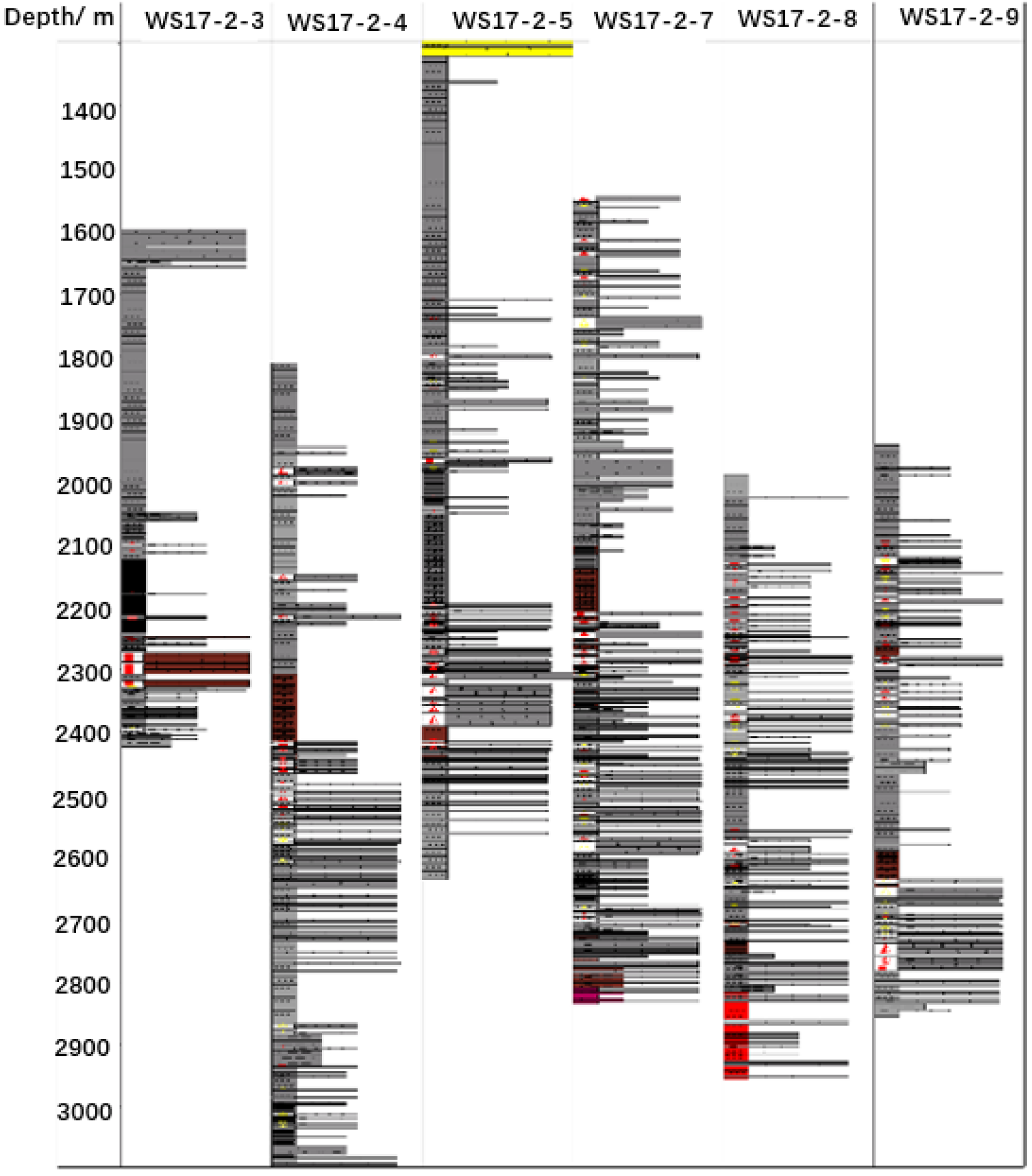
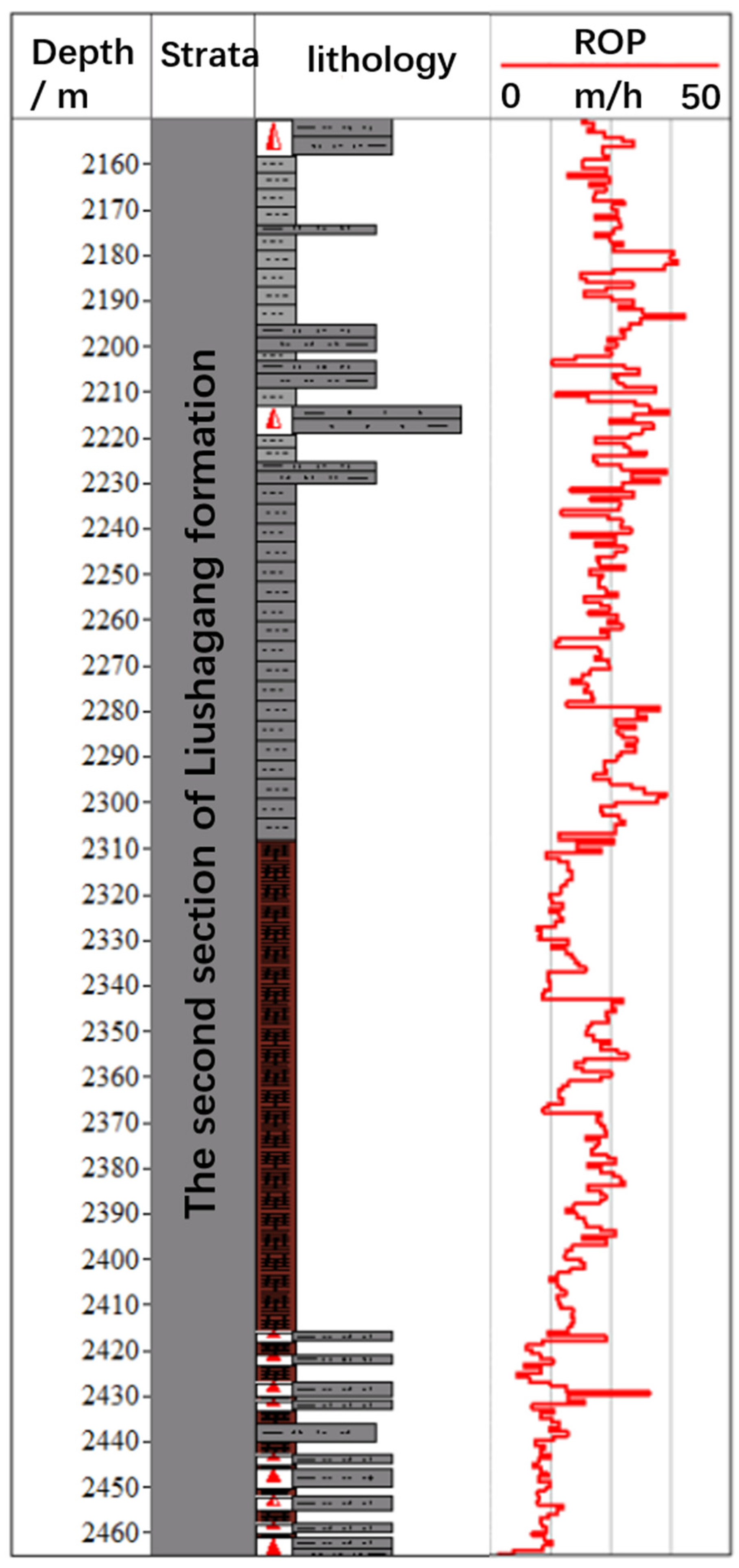
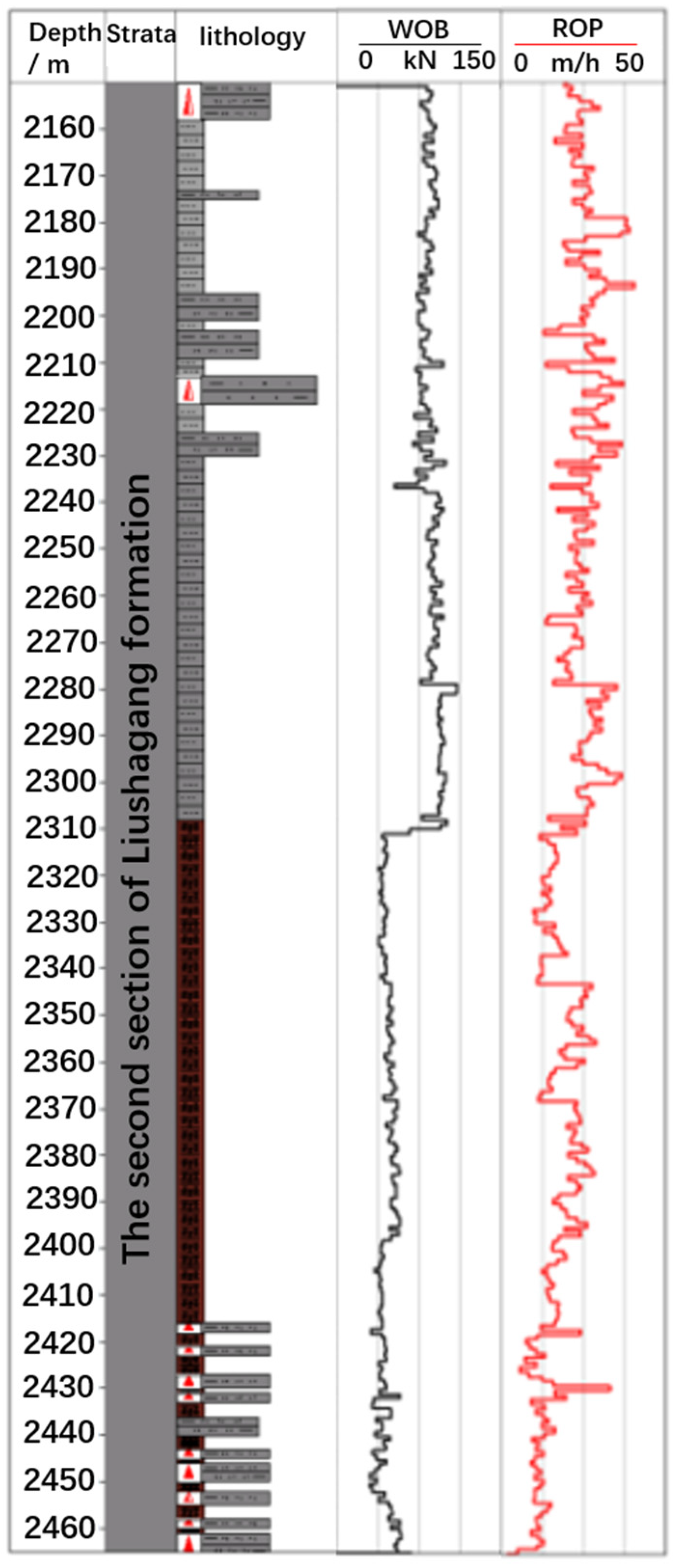
2. Stratigraphic Profiles

Wushi 17-2 block is located in the east of Wushi Sag in Beibu Gulf Basin of the South China Sea with extremely rich reserves of intensified oil and gas resources [23]. However, as a typical fault block reservoir, the lithology of Liushagang Formation is considerably complex, where the mudstone, sandstone and shale are unevenly distributed in the thick mixed layers [24,25,26]. Most of the formation rocks present with high argillaceous and strong water sensitivity. Meanwhile, the drillability of the mudstone formation is poor, and the rock strength of the sandstone and gravel formation is high with strong abrasiveness. When the PDC bit drills in such soft–hard intersected layers, some of the drilling parameters such as WOB and rotational speed cannot fully match the rock properties, resulting in efficiency reduction of the bit in the rock breaking and a generally low ROP. According to the field data, the average ROP of seven early exploratory wells in the upper formation was 87.32 m/h, while the average ROP of the Liushagang Formation was only 23.27 m/h, which was 73% lower than that of the upper formation (see Figure 1). Considering the high cost of offshore drilling and severe working conditions, the development of a suitable ROP prediction model for the Liushagang Formation would be an important and theoretical guidance for drilling parameter adjustment, ROP improvement and drilling period reduction during the whole construction process.

3. Controlling Factors of ROP

3.1. Stratigraphy

The characteristics of rock which strongly affect ROP are of inherent nature of the target formation and thus cannot be changed. Figure 2 shows the lithology profile of the Liushagang Formation. According to the lithology distribution law, the Liushagang Formation can be divided into an upper homogeneous mudstone and sandstone section, and the middle and lower soft-hard interlaced section. The middle and lower formations are mainly dominated by mudstone with a small amount of sandstone and shale. The average proportion of mudstone, sandstone and shale in the Liushagang Formation is 62.82%, 24.95% and 11.23%, respectively. Based on the whole-rock mineral X-ray diffraction (XRD) analysis, the content of clay mineral of this formation is around 45%.

ROP is mainly controlled by the lithology of formation. When drilling in the upper homogeneous formation, the ROP can maintain at a relatively high value, while for the soft-hard intersected layers in the middle and lower section, due to the significant variation in lithology and the strong fluctuation of WOB, the ROP would be hard to be maintained in a stable manner and the ROP is relatively low.

Figure 3 shows the strength envelope using Mohr–Coulomb criterion from the rock mechanics experiments on core samples from the field [27]. The results indicate that the rock cohesion force of the target formation is 6–8 MPa, implying a poor cementation with a loose rock structure.

3.2. Drilling Parameters

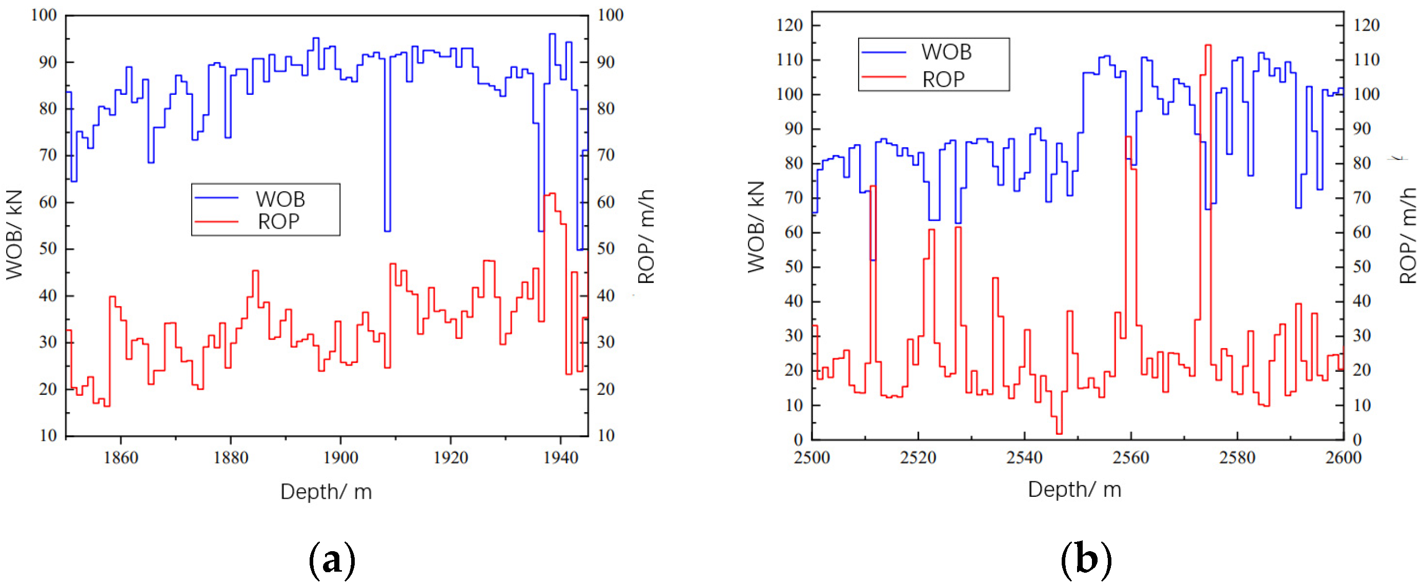
The drill bits used in the formation we studied in this work was PDC bits with a size of 12 1/4in. PDC bits mainly rely on chamber plows in soft formations and cutting in hard formations. When the cutting depth is relatively shallow, the rock is mainly plastically damaged, which is represented by the continuous accumulation of powder particles at the tip of the tool. When the cutting depth reaches a certain value, the rock will suffer brittle failure, which is manifested as cracks extending from the tool tip along the cutting direction, and finally extending to the free surface to form larger chips.

3.2.1. WOB

The relationship between ROP and WOB in the upper and lower formations of the Liushagang Formation are different. Taking the section of the Liushagang Formation in well X-2 for example (Figure 4): in the upper homogeneous formation, increasing WOB increases ROP; however, in the lower soft and hard staggered formation, increasing WOB leads to a decrease in ROP.

3.2.2. Rotating Speed

In the drilling industry, the wellhead rotary table drives the drill pipe and lower part of the drilling tool to rotate. The rotation speed of the rotary table highly depends on the efficiency of rock breaking. Therefore, the rotation speed is one of the key drilling parameters that affects the mechanical penetration rate. Given the complex working conditions during the actual drilling process, it is essential to have a good analysis to characterize the relationship between the rotating speed and ROP at different drilling conditions.

Figure 5 shows the variation in ROP and rotation speed at the depth from 1900 to 1990 m in the Liushagang Formation of well X-2. In general, the rotational speed of the whole section remains relatively stable. At a depth of 1940 m, the rotational speed starts to decrease. At the same section, the ROP presents an obvious low value, indicating a strong dependence between ROP and rotation speed. During the normal drilling process in the Liushagang Formation, a lower speed can lead to the reduction in ROP. For the well section with stable rotating speed, the complex operating conditions such as drilling in soft-hard intersected layers or other drilling parameter fluctuations can also cause the ROP fluctuation.

3.2.3. Pump Volume

Rock cuttings broken by the bit cutting teeth usually need to be removed from the bottom of the well to avoid repeated bit breaking [28]. To effectively remove the formed cuttings, drilling fluid is commonly used. A proper pump volume of drilling fluid can ensure a good migration of rock cuttings and also save the cost of drilling. Figure 6 shows the design and actual drilling pump volume data of four wells. To guarantee the effective cleaning of the well bottom, the recommended pump volume is 3000–3200 L/min.

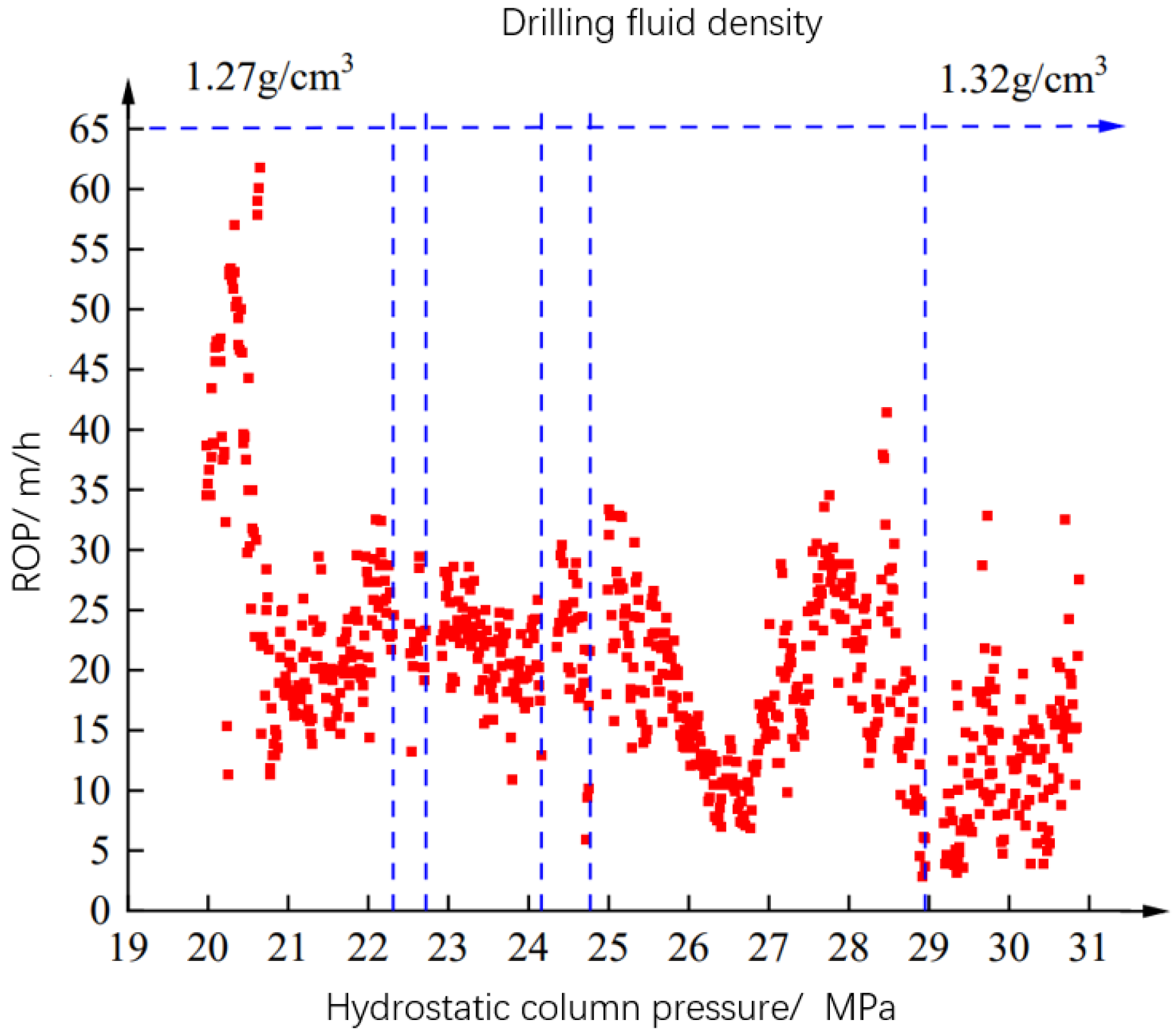
3.2.4. Drilling Fluid Density

Drilling fluid is considered as the “blood” in drilling engineering and plays the role of bridge between the ground and underground [29]. A suitable drilling fluid density can effectively balance the pressure during drilling and avoid circulation loss or wellbore instability. Figure 7 shows the variation in ROP and hydrostatic column pressure with consideration of drilling fluid density in well X-1. In general, increasing drilling fluid density decreases the ROP.

3.3. Drilling Tool

There are many types of downhole tools, including hydraulic oscillators to ensure WOB transmission, and centralizers to avoid drill pipe bending [30,31,32,33]. In this work, we only discuss the influence of the bit on ROP. As the main tool for rock breaking, the wear of the bit cutting teeth is highly related to drilling efficiency. With the same values of other parameters, the greater the wear degree of the cutting teeth, the smaller the volume of rock breaking, and the lower the ROP [34]. It is worth noting that other drilling tool parameters, such as the bit tooth distribution mode, tooth shape and number of teeth, can also affect the ROP [35].

According to the statistics from the field, the bit’s cutting tooth used in the Liushagang Formation shows more or less wear. The average wear of the inner cutting tooth is 29.7%, and the average wear of the outer cutting tooth is 54.7%. In this work, considering the different usage and different degree of bit with various types, a constant value is set in the ROP prediction model.

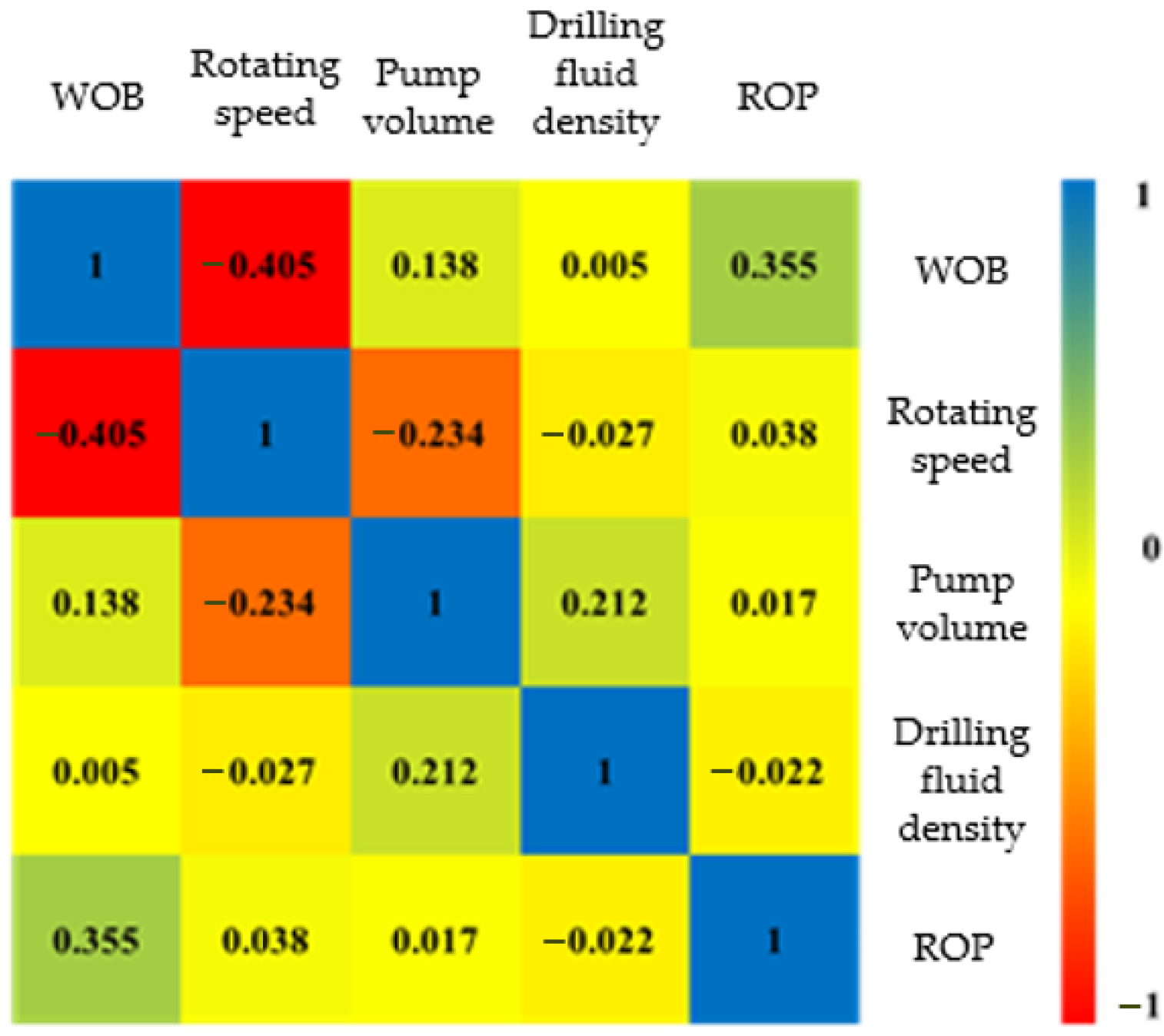
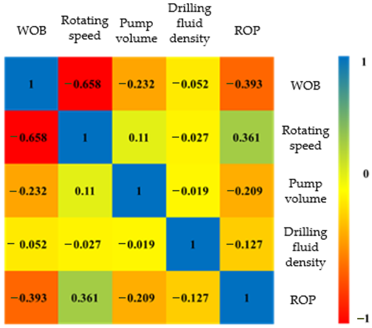
3.4. Analysis of Main Controlling Factors

To analyze the controlling factors of ROP, based on the drilling data collected from the field, we used a correlation analysis method to interpret the relationship among lithology, WOB, rotating speed, pump capacity, drilling fluid density and ROP. The thermal diagram of the main controlling factors is shown in Figure 8, Figure 9 and Figure 10. In these figures, the blue blocks represent a positive correlation and the red represent a negative correlation. It is clear to see that the drilling parameters at different sections show different influence on ROP.

The main controlling factors governing ROP and the recommended drilling parameter interval in the Liushagang Formation are shown in

Table 1. Recommended range of main control factors of ROP.

Stratum	Main Control Factors	Recommended Range
Section 1 of Liushagang Formation and upper part of Section 2 of Liushagang Formation	Rotating speed Drilling fluid density	[110, 120] r/min [1.33, 1.35] g/cm3
Lower part of Section 2 of Liushagang Formation	WOB	[60, 90] kN
Section 3 of Liushagang Formation	WOB Rotating speed	[70, 90] kN [100, 120] r/min

. These drilling parameters need to be taken into account when developing an ROP prediction model. When optimizing drilling parameters, it is necessary to adjust the relative parameters based on these controlling factors at different layers to ultimately achieve an effective ROP release.

4. A Prediction Model of ROP Based on DNN

The deep neural network contains multiple intermediate layers. Except for the input and output layer, all intermediate layers are the hidden layers. The connection mode between different layers is full connection. Therefore, DNN is also called the full connection neural network [36].

Compared to the traditional method, DNN has high accuracy and strong robustness. It plays an important role in the field of data mining. For the complex drilling process, DNN has great potential to address the large number of data processing because of the fast calculation speed, flexible structure and convenient implementation [37]. The simple topology of DNN is shown in Figure 11.

4.1. Design of ROP Prediction Model

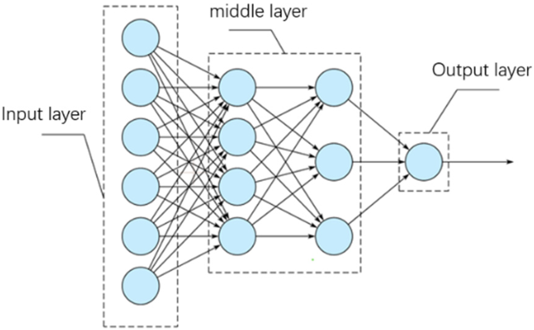
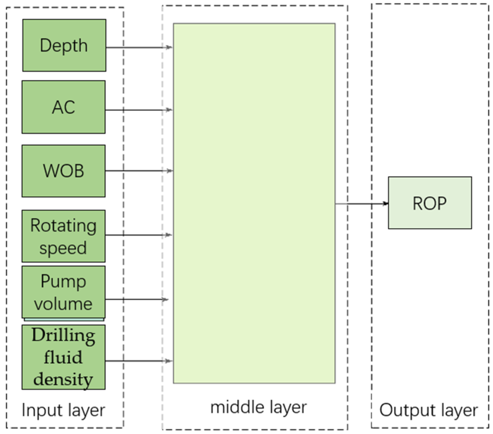
4.1.1. Input Layer, Middle Layer and Output Layer Selection

Based on the aforementioned analyses on the factors affecting the ROP of the Liushagang Formation, we chose the depth, formation lithology, WOB, rotating speed, pump volume and drilling fluid density as the input parameters of DNN, and ROP as output terminal, which is illustrated in Figure 12. The middle layer was set to two layers, and each layer has 64 neurons. For formation lithology, the traditional rock cuttings judgment method is not suitable for the actual field operation anymore, and it is extensively affected by the experience. The acoustic moveout data can reflect the changes of rock dynamic elastic parameters and represent the strength characteristics of the formation to a certain degree. Therefore, the acoustic time data was selected as the lithology substitute value input. The acoustic time difference data of new wells can be obtained by inversion of block seismic data [38].

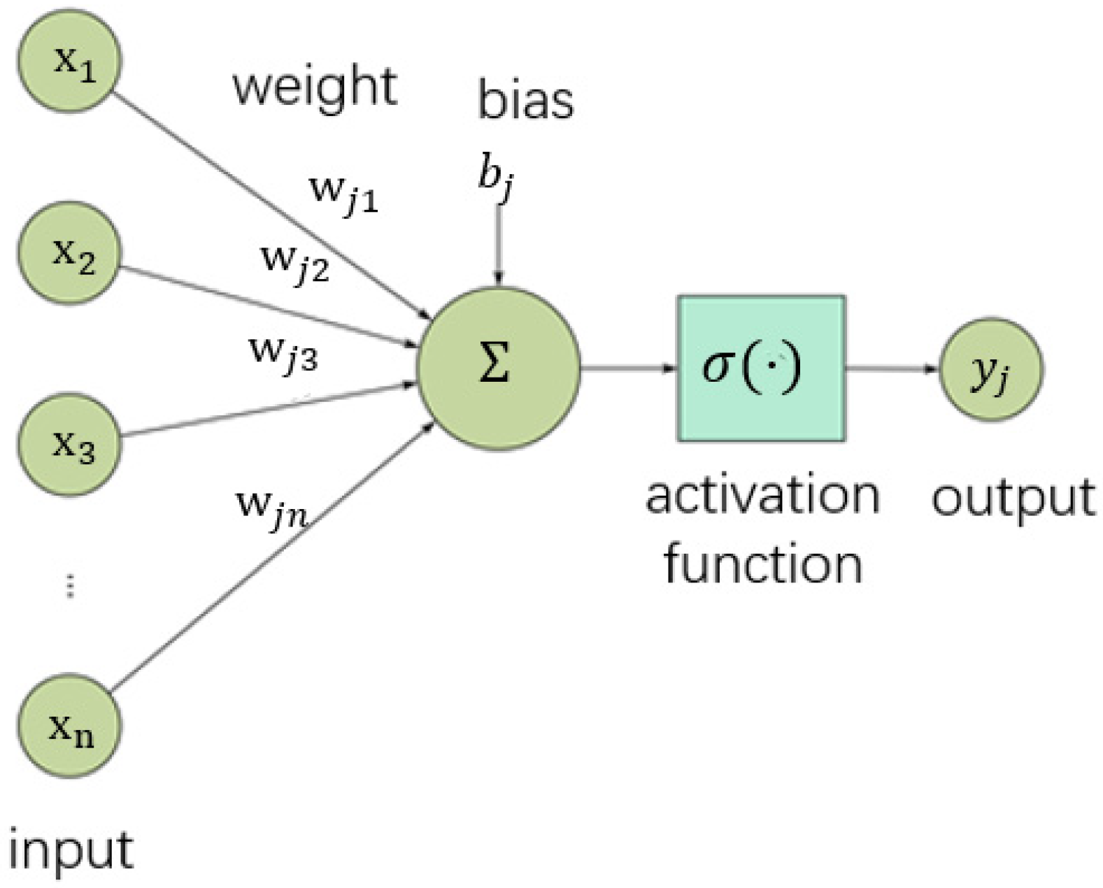
4.1.2. Weights, Bias and Activation Function Settings

The basic structure of the neurons in DNN consists of weight, bias and activation function. The weight represents the connection strength of two neurons in adjacent layers. The bias can translate the activation function. The activation function endows the network with the ability to address nonlinear problems and limits the output amplitude of neurons to a specified range, which is generally limited to (−1, 0) or (0, 1). Figure 13 shows the neuron structure.

Assuming that a DNN has X layers, where the first layer and layer X are the input and output layer, respectively, the remaining X-2 layers are therefore intermediate layers. In this case, any layer n (1 < n ≤ X) would satisfy the following equation:

$$f_{input p}^{ n}={{\displaystyle \sum }}_{q=1}^{sum\left(n-1\right)}{\omega }_{pq}^n{f}_{input q}^{ n-1}+b_p^n nϵ\left[2,X\right]$$

(1)

$$f_{output p}^{ n}={\sigma }_n\left(f_{input p}^{ n}\right)$$

(2)

where $f_{input}^{ n}$ and $f_{output}^{ n}$ is the input and output of the p-th neuron in layer n; ${\omega }_{pq}^n$ is the weight between the q-th neuron in layer n − 1 and the p-th neuron in layer n; $b_p^n$is the bias of the p-th neuron in layer n; ${\sigma }_n(·)$ is the activation function; $sum\left(n-1\right)$ is the total number of neurons in layer n − 1.

The specific settings of the weights, biases and activation function of the neural network model are shown in

Table 2. Settings of the weights, biases and activation function.

Name	Setting
Weights	normal distribution
Bias	0.1
Activation function	ReLU

.

4.1.3. Adam Optimizer

Different types of optimizers have different convergence rates. Considering the influence of certain randomness during the drilling process and to avoid falling into local minimum and inability to achieve global optimization, in this work, Adam optimizer is selected as the optimizer of the ROP prediction model.

Adam optimizer was proposed by Kingma et al. in 2014 [39], and the expression is given by:

$${\theta }_{1+t}={\theta }_t-\frac{\eta }{\sqrt{\widehat{v_t}+ϵ}}\widehat{m_t}$$

(3)

where $\widehat{v_t}$ is the exponential decay average of the historical square gradient; $\widehat{m_t}$ is the exponential decay average of the historical gradient.

The Adam optimizer can automatically adjust the learning rate, which would not be affected by the change of historical gradient scaling. For drilling engineering with a large number of data and parameters, the Adam optimizer is convenient to implement and has a small amount of calculation, which is quite suitable for the optimization of the ROP prediction model.

4.1.4. Dropout Mechanism

During the DNN training process, it is common to face the overfitting problem where the fitting degree of training set data is too high with a poor fitting result of the test data. The overfitting issue usually occurs when the gap between the training set and the test set is large. Due to the complexity of the drilling, there might be a big difference between the training set data and the test set data, which may trigger overfitting errors. If the overfitting problem is not solved, the ROP prediction result would greatly deviate from the actual situation, and lead the trained ROP model to certain meaninglessness.

Dropout is an update method that can effectively prevent overfitting problems [40]. The principle of dropout is that, in the process of forward data transmission, some neurons are stopped randomly. This process changes the structure of the neural network, and the model would be no longer dependent on any group of neurons. Therefore, all neurons will be accounted for to avoid falling into local optimization. The schematic of dropout is shown in Figure 14. Meanwhile, the additional dropout can strengthen the ability of neurons and reduce the cost of training. In a real application, if the set value is too low, the dropout would not enhance the generalization ability. On the other hand, if the set value of dropout is too high, it would lead to underfitting. After comprehensive consideration, in this work, the dropout value of this model was set to 0.25.

4.1.5. L2 Regularization

During the neural network training, the weight coefficient between neurons has a great impact on the calculation output. Excessive weight coefficient will lead the neural network to rely on the excessive weight of the training set. If the error between the training set and test set is high, when the test set data is brought into the trained network to validate the network generalization ability, the fitting result of the training set would deviate too much from the real value. To ensure a suitable value of weight, it is reasonable to apply L2 regularization for adding constraints on parameters.

The principle of L2 regularization is to penalize the peak weight vector by adding the sum of the squares of all the weight values of the neural network to the loss function, so that the network can account for the weight vector, avoid falling into local optimum, and improve the generalization ability of neural network models. During the gradient descent stage, the essence of L2 regularization is to attenuate the weight of each neuron to 0 using the equation given by:

$$R_{\omega }=\frac{1}{2}\lambda {\Vert \omega \Vert }_2^2$$

(4)

where: ${\Vert \omega \Vert }_2^2$ is 2-norm square term of $\omega$; $\lambda$ Is the regularization coefficient.

Taking the above formula into the loss function, the final result is given by:

$$Loss=Los{s}_0+\frac{\lambda }{2n}{{\displaystyle \sum }}_{\omega }{\omega }^2$$

(5)

where $Los{s}_0$ is the original loss function; $\frac{\lambda }{2n}{{\displaystyle \sum }}_{\omega }{\omega }^2$ is the sum of squares of all weights which is quantitatively adjusted by $\frac{\lambda }{2n}$; n is the number of instances contained in the training set.

From Equation (5), it can be found that the regularization process is actually the allocation and adjustment of small weight to minimize the original loss function. The larger the regularization coefficient, the more the network tends to pursue small weight. On the other hand, the smaller the regularization coefficient, the higher the degree of the network minimizing the original loss function.

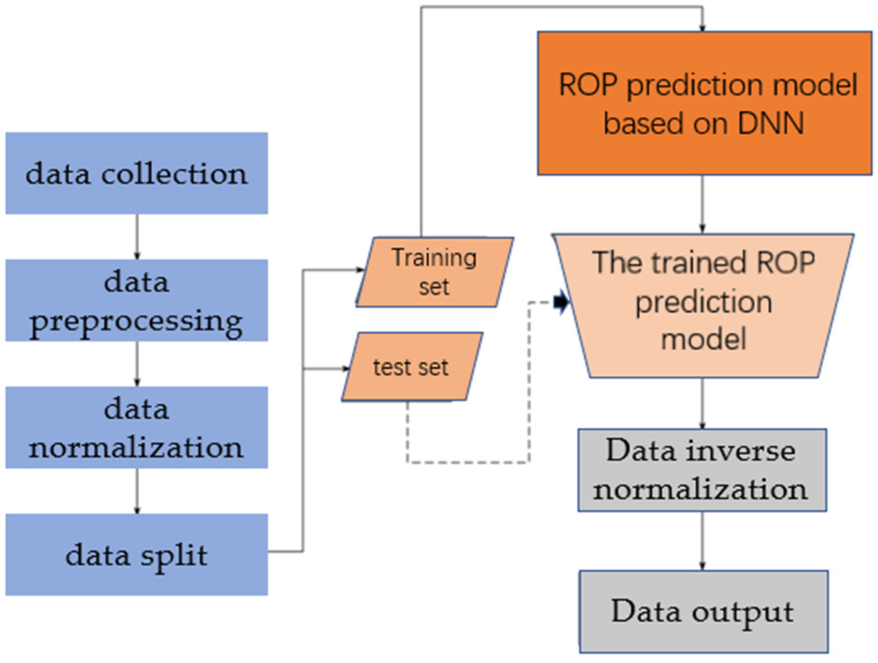
4.1.6. Calculation Process

The ROP prediction model provides an end-to-end calculation process through the DNN. From the inputs such as acoustic time difference, drilling, hydraulic parameters and other data to the outputs to predict the ROP, the whole calculation process can be decomposed into drilling data cleaning (removing outliers), drilling data normalization, input drilling data, data transfer between the input layer and middle layer, establishment of mapping relationship between the middle layers, prediction data as the output layer, data inverse normalization processing and other steps. The calculation workflow diagram is shown in Figure 15. The specific steps are listed as follows:

• Data collection: collect acoustic time, drilling parameters, hydraulic parameters and ROP data.
• Data preprocessing: clean the collected data and fill the missing points with the average value.
• Data normalization: to coordinate the size of different parameters; for example, the numerical range of pump volume is 2000~3500, while the drilling fluid density range is mostly 1.3~1.4. The difference between the two is too large. In order to avoid the calculation error caused by the large gap between the data, as well as the problem of memory usage and slow calculation, the data is normalized.
• Data loading: input the processed data into the DNN.
• Nonlinear mapping: The DNN completes the nonlinear mapping calculation from the input layer to the output layer.
• Data inverse normalization: inverse normalization of output layer data.
• Data output: output the predicted ROP.

4.2. ROP Prediction Model Training

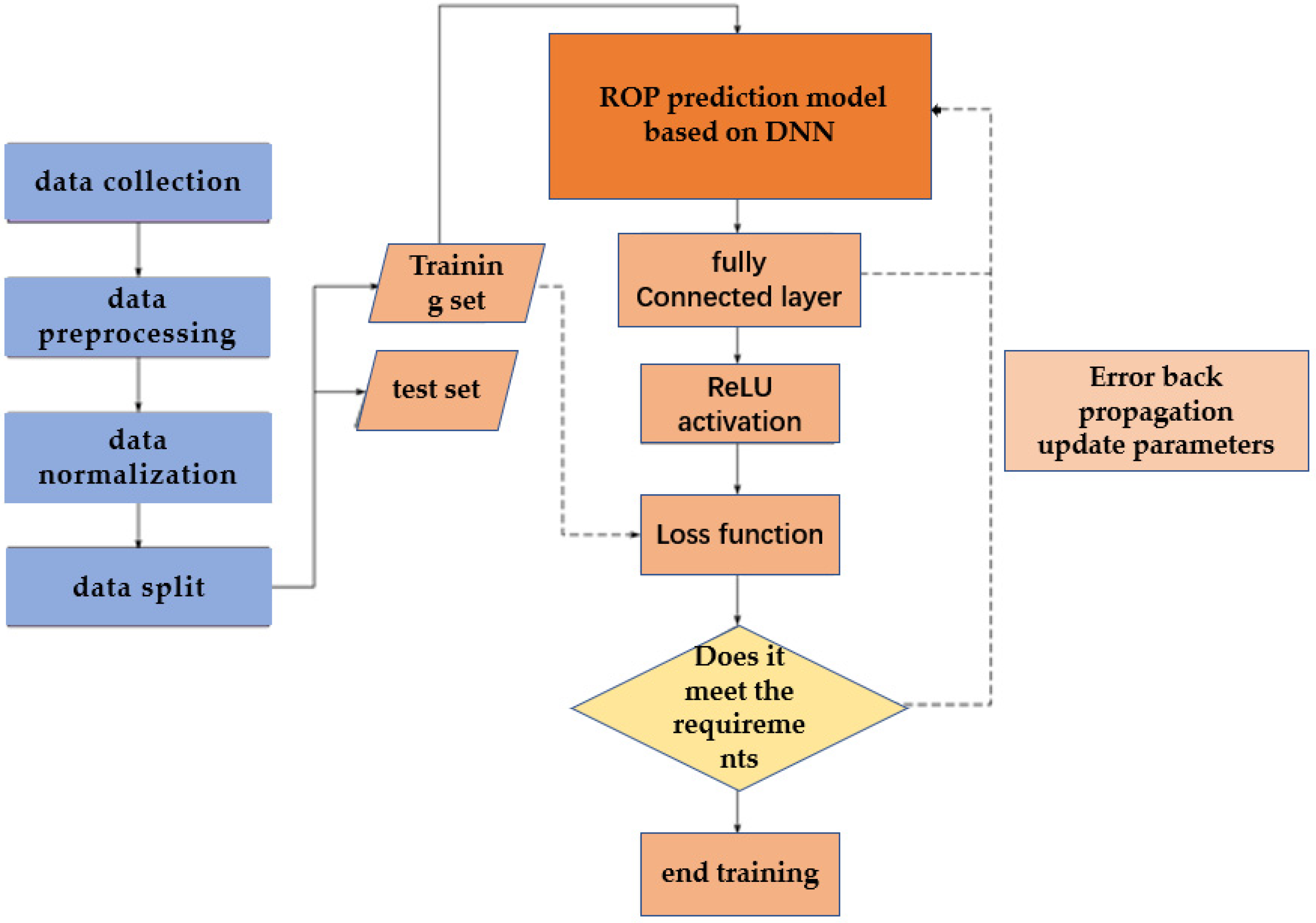
4.2.1. Training Process

In general, there are two data transmission modes in the DNN ROP prediction model: forward propagation and back propagation. The forward propagation mode is the process of establishing a nonlinear mapping from the input to output terminal, whereas the back propagation mode uses the loss function to calculate the partial derivatives of different parameters, and then updates the weights of different parameters. When the convergence loss function of the ROP prediction model meets the preset accuracy or the ROP prediction model reaches the maximum iterations, the training will be stopped. The specific ROP training process is illustrated in Figure 16:

From Figure 17, before the iteration, the training model of ROP prediction needs to complete several data processing steps, including preprocessing, normalization and splitting of drilling data, to ensure the reliability of the data involved in training and testing. The split training set is used to verify the loss function of the ROP prediction model and calculate the parameter gradient. When the calculation results cannot meet the end conditions, data back propagation will occur, and the weight parameters between different layers will be updated for the second iteration.

4.2.2. Training Data Split

In order to obtain an ROP model that meets industry requirements, the data were divided into training set and test set. The training set was used for training the ROP prediction model. During the training on the training set, the DNN continuously updates the iterative parameters based on the training set data characteristics and errors. The test set was used for verifying whether the trained ROP model had good generalization ability or not.

In this paper, the data from four wells are classified and divided into input and output data with consideration of the structure of the ROP prediction model. Three wells were used as the training set and one well was used as the test set. The data splitting of these wells is shown in

Table 3. Data splitting for training and test set.

Test Well	Original Dataset	Training Set	Test Set
X-1	4155	3373	782
X-2	4155	2974	1181
X-3	4155	2908	1247
X-4	4155	3210	945

. The aim of data splitting is to avoid the poor fitting result of the ROP prediction model due to limited data.

4.2.3. Training Strategy

The training of the DNN ROP prediction model is a process where the weights of parameters between different layers are continuously optimized and adjusted with the iteration, and ultimately meet the expected training results. Before training the network, it was necessary to set up the input and output terminals of the network and prepare training data. At the beginning of training, the initial weight of the network needs to be given. During network training, the network will automatically update the weight based on the preset sample batch size, sample iteration epochs, learning rate, learning rate decay rate and other super parameters, so as to subsequently make the regression fitting results meet the requirements, and to establish the nonlinear function mapping of input and output. The specific super parameter settings of ROP prediction model training are shown in

Table 4. Hyperparameter design.

Hyperparameters	Setting
batch size	100
epoch	100
learning rate	0.003
learning rate decay rate	0.15

:

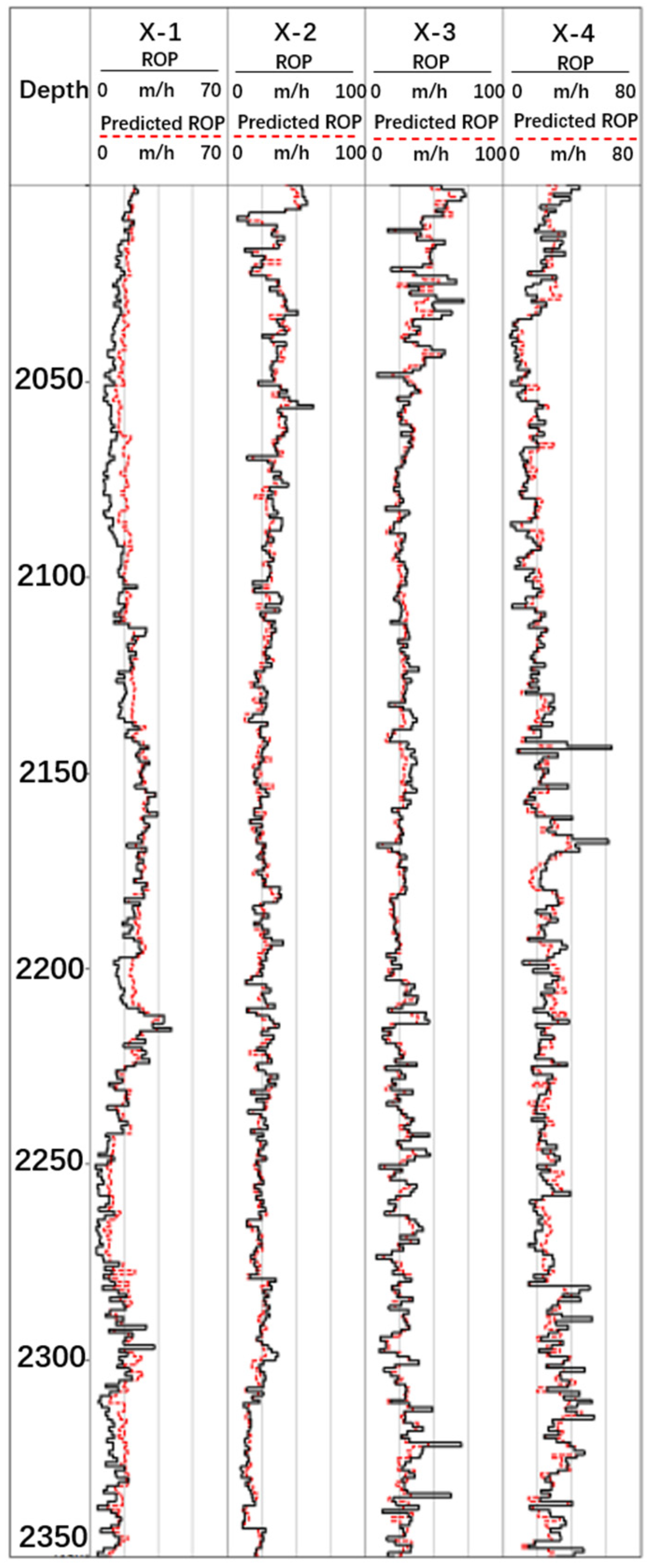
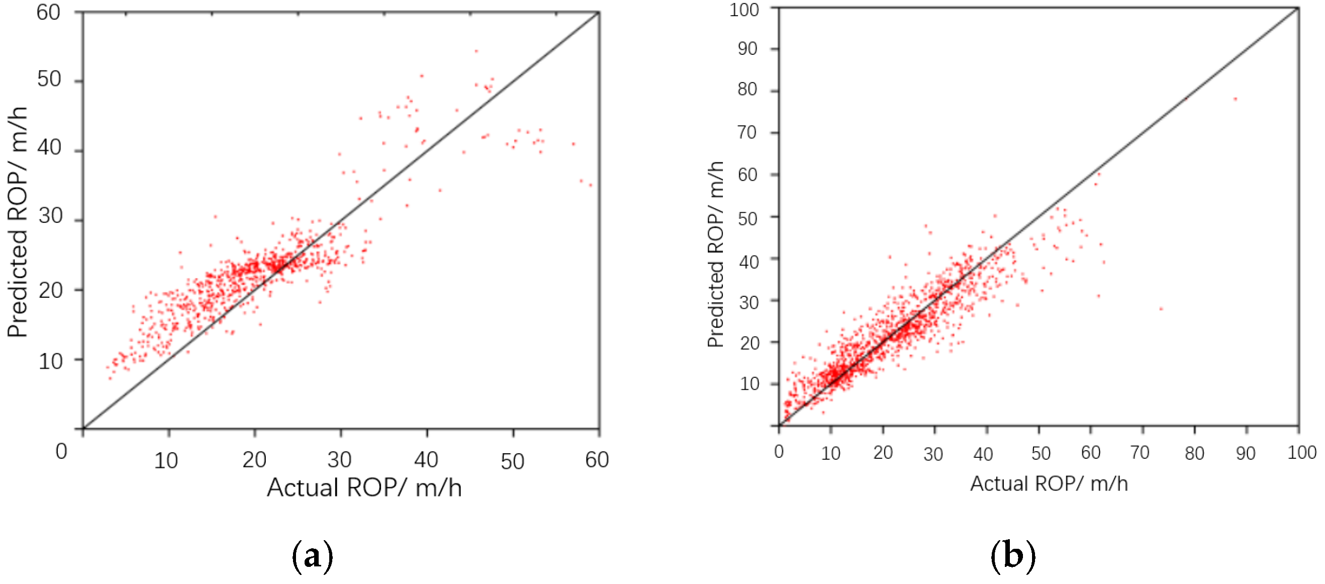
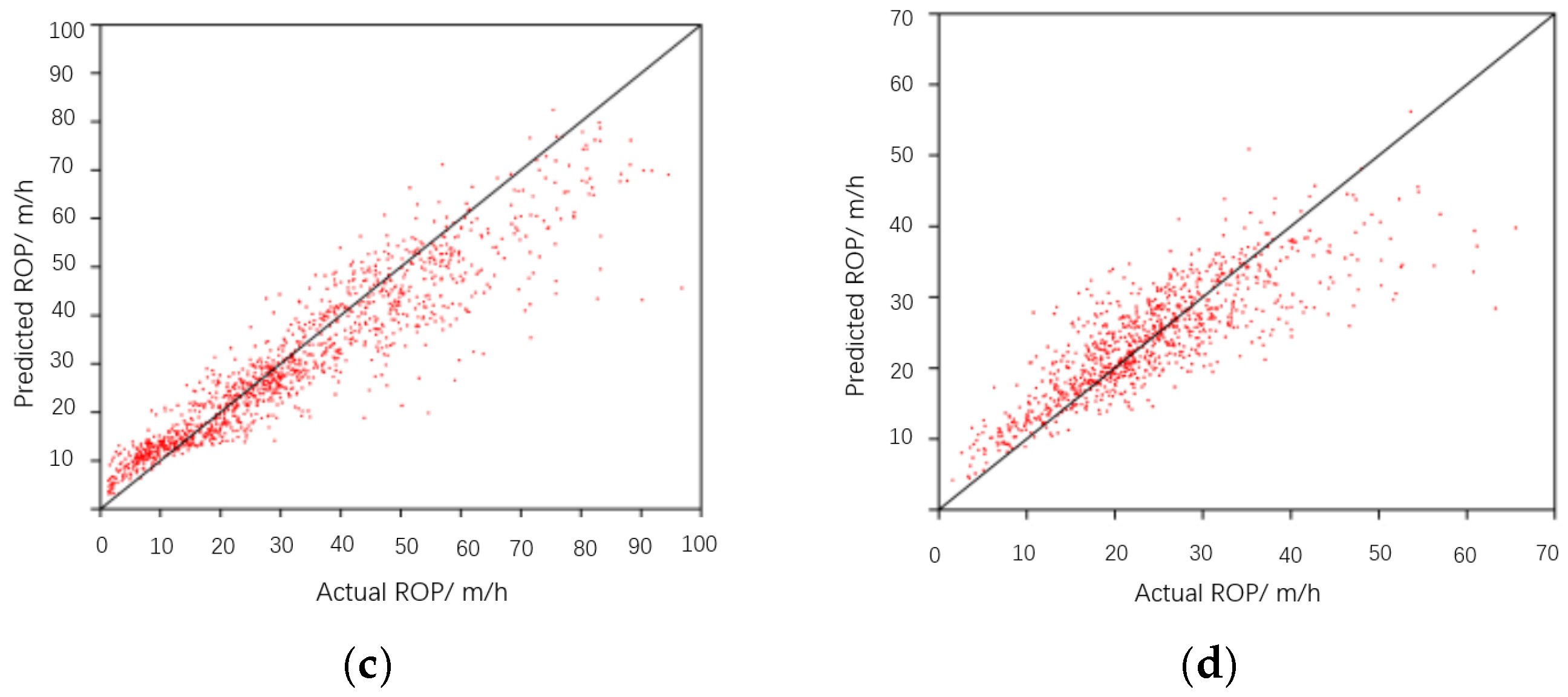
4.3. Generalization Ability Test of ROP Prediction Model

After model training, the generalization ability of the ROP prediction model was tested using the split test set data. The design parameters of the test wells were selected as inputs for the network, and the calculated predicted ROP was used as the output. Figure 17 shows the predicted ROP based on the DNN model and the real ROP as function of depth for the four exploration wells. The black line in the figure represents the actual ROP, and the red line represents the predicted ROP. According to the curve fitting results of these wells, our ROP prediction model shows strong ability for nonlinear function fitting.

The prediction performance of four independent wells as test sets is shown in Figure 18. The average R² between the real and predicted ROP of the four wells is 0.82. Furthermore, the average relative error between the predicted and real ROP of the four wells is shown in

Table 5. Relative error of multi-well prediction results.

Well	Test Data	Average Relative Error
X-1	782	16.59%
X-2	1181	14.06%
X-3	1249	15.32%
X-4	945	14.95%

. The average relative error of the predicted ROP of the four exploration wells is 15.23%.

5. ROP Predictive Model Applications

The prediction model of ROP developed in Section 4 presents good generalization ability after being verified by the training set. To better test and validate this established model, it is worthwhile applying it for a field simulation. In this section, the middle and lower formation of Section 2 of the Liushagang Formation in well X-2 in Wushi 17-2 block is used as an example for further validation.

5.1. Geological Profile

Well X-2 is located in the north of Wushi 17-2 block. The stratum depth in the middle and lower part of Section 2 of the Liushagang Formation is about 2151–2465 m. The lithology of this stratum is mainly gray mudstone and brownish gray shale, accompanied by a small amount of gray siltstone. When drilling into the shale formation at a depth of 2310 m, there is an obvious ROP reduction. Based on the field data (Figure 19), the average ROP at the depth from 2310 to 2410 m was only 18.42 m/h, while the average ROP of 2151–2309 m was 25.51 m/h, which gives a 28% decrease.

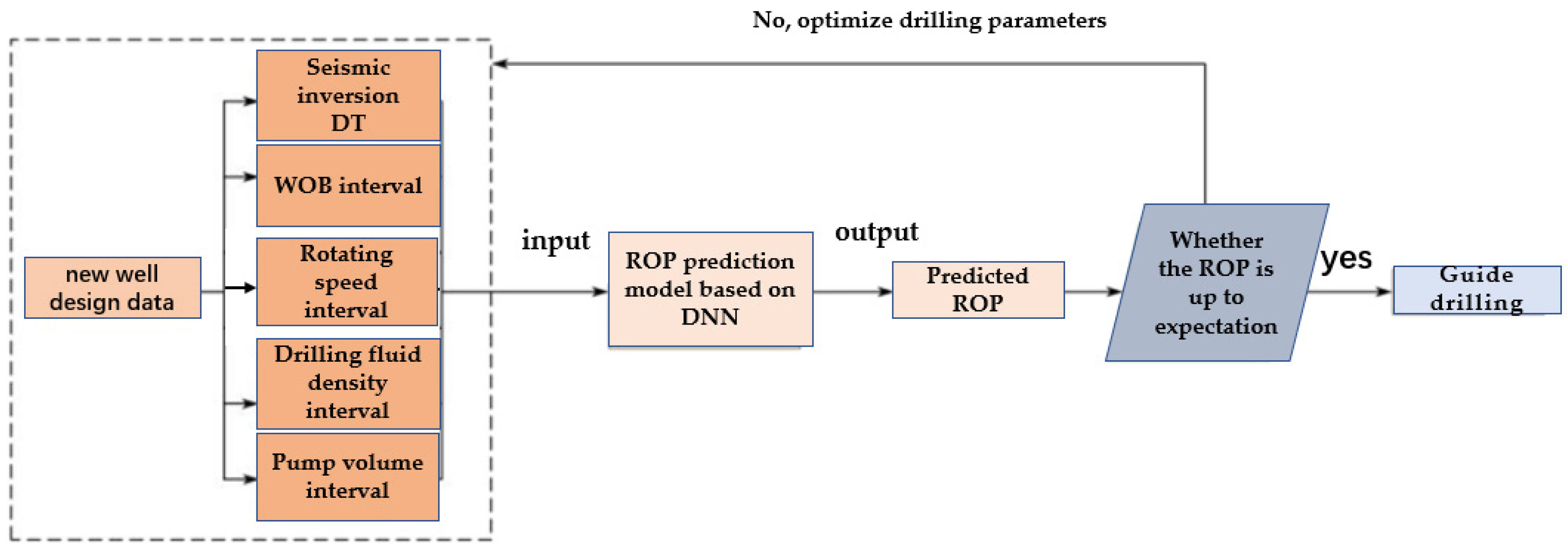
5.2. Drilling Parameter Optimization Process

With consideration of the analysis of the main controlling factors on ROP in Section 3 and the DNN ROP prediction model established in Section 4, we developed a comprehensive framework for drilling parameter optimization (Figure 20). The main steps consist of:

• Collection of design data of new well: use seismic method to invert the acoustic time data in the new well of the Liushagang Formation, and find the drilling parameter interval based on the design data of the new well and the history data of the completed adjacent wells.
• Prediction of ROP: take the design data as the input of the model and bring it into the DNN ROP prediction model for prediction.
• ROP judgment: the field operator judges whether the predicted ROP results meet the engineering expectations.
• Drilling parameter optimization: adjust the drilling parameters of the well section where the predicted ROP does not meet the engineering expectations, and adjust the main control factors according to the analysis results of the factors affecting the ROP in different layers of the Liushagang Formation.
• Re-prediction of ROP: the adjusted drilling parameters and unknown variables are taken as the input of the model and brought into the ROP prediction model based on DNN for prediction.
• Guide drilling: after the predicted ROP meets the actual engineering expectations, drill with the optimized drilling parameters.

After the analyses of the main controlling factors on ROP in the middle and lower part of the Liushagang Formation (detailed in Section 2), WOB was identified as the main dominating parameter. Figure 21 shows the profile of lithology, WOB and ROP vary with depth. It can be found that WOB starts to decrease at a depth of 2310 m. The average WOB at the depth from 2310 to 2410 m is 47.08 kN, whereas the average ROP is only 18.42 m/h. Therefore, adjusting WOB of this well section can clearly improve the ROP performance while keeping other parameters as constants. The recommended WOB is 80 kN.

The next step is to bring the optimized drilling parameters into the ROP prediction model, and acquire the optimized predicted ROP results by calculating output. A comparison between the actual ROP, the predicted ROP and the optimized predicted ROP is shown in Figure 22. From the figure, it is found that the predicted average ROP increases to 27.67 m/h after a pressure increase compared to the initial WOB of only 18.42 m/h. Generally, after WOB optimization at a depth of 2310–2410 m of well X-2 in the Liushagang Formation, the ROP performance is clearly improved. Therefore, our drilling parameter optimization process based on the DNN ROP prediction model can guide the drilling parameter adjustment operation in the field.

6. Conclusions

In this work, we show a novel ROP prediction model based on a deep neural network. Using the drilling data of Wushi 17-2 block in the South China Sea, we characterize the controlling factors on ROP of the Liushagang Formation through the developed model. The main conclusions are summarized as follows:

• The ROP of the Liushagang Formation is mainly affected by stratigraphic lithology, and the controlling parameters on ROP are highly related to stratigraphic properties.
• The prediction model of ROP based on DNN shows good generalization ability and can meet the requirement of drilling engineering with a high enough accuracy.
• We also developed a framework or workflow for drilling parameter optimization. This workflow was validated by the simulation using data from the real field, and it can guide the optimization of drilling parameters to effectively improve the drilling speed.
• Compared with other data-driven ROP prediction models, the model developed in this work takes the formation conditions into account, and the prediction accuracy in complex formations can meet the requirements. However, the formation situation is more complex, and it is far from enough to replace the formation situation with the acoustic transit time only. Other parameters need to be added to the model to better describe the formation.

References

1. Astakhov, V.P. Chapter 12—Drilling. In Modern Machining Technology; Paulo Davim, J., Ed.; Woodhead Publishing: Sawston, UK, 2011; pp. 79–212. [Google Scholar]
2. Maurer, W.C. The “perfect-cleaning” theory of rotary drilling. J. Pet. Technol. 1962, 14, 1270–1274. [Google Scholar] [CrossRef]
3. Bingham, G. A new approach to interpreting rock drillability. Tech. Man. Repr. Oil Gas J. 1965, 93 P, 1965. [Google Scholar]
4. Bourgoyne, A.T., Jr.; Young, F.S., Jr. A multiple regression approach to optimal drilling and abnormal pressure detection. Soc. Pet. Eng. J. 1974, 14, 371–384. [Google Scholar] [CrossRef]
5. Warren, T.M. Penetration rate performance of roller cone bits. SPE Drill. Eng. 1987, 2, 9–18. [Google Scholar] [CrossRef]
6. Hareland, G.; Rampersad, P.R. Drag-bit model including wear. In Proceedings of the SPE Latin America/Caribbean Petroleum Engineering Conference, Buenos Aires, Argentina, 27–29 April 1994. [Google Scholar]
7. Motahhari, H.R.; Hareland, G.; James, J.A. Improved drilling efficiency technique using integrated PDM and PDC bit parameters. J. Can. Pet. Technol. 2010, 49, 45–52. [Google Scholar] [CrossRef]
8. Mendes, J.R.P.; Fonseca, T.C.; Serapião, A.B.S. Applying a neuro-model reference adaptive controller in drilling optimization. World Oil Mag. 2007, 228, 29–38. [Google Scholar]
9. Soares, C.; Daigle, H.; Gray, K. Evaluation of PDC bit ROP models and the effect of rock strength on model coefficients. J. Nat. Gas Sci. Eng. 2016, 34, 1225–1236. [Google Scholar] [CrossRef]
10. Bilgesu, H.I.; Tetrick, L.T.; Altmis, U.; Mohaghegh, S.; Ameri, S. A new approach for the prediction of rate of penetration (ROP) values. In Proceedings of the SPE Eastern Regional Meeting, Lexington, Kentucky, 23–25 October 1997. [Google Scholar]
11. Moran, D.; Hani, I.; Purwanto, A. Sophisticated ROP prediction technologies based on neural networks delivers accurate drill time result. In Proceedings of the SPE Asia Pacific Drilling Technology Conference and Exhibition, Ho Chi Minh City, Vietnam, 1 November 2010. [Google Scholar]
12. Al-Abduljabbsr, A.; Elkatatny, S.; Abdulhamid Mahmoud, A.; Moussa, T.; Al-Shehri, D.; Abughaban, M.; Al-Yami, A. Prediction of the Rate Penetration while Drilling Horizontal Carbonate Reservoirs Using a Self-Adaptive Artificial Neural Network Technique. Sustainability 2020, 12, 1376. [Google Scholar] [CrossRef] [Green Version]
13. Moraveji, M.K.; Naderi, M. Drilling rate of penetration prediction and optimization using response surface methodology and bat algorithm. J. Nat. Gas Sci. Eng. 2016, 31, 829–841. [Google Scholar] [CrossRef]
14. Amer, M.M.; Dahab, A.S.; El-Sayed, A.-A.H. An ROP Predictive Model in Nile Delta Area Using Artificial Neural Networks. In Proceedings of the SPE Kingdom of Saudi Arabia Annual Technical Symposium and Exhibition, Dammam, Saudi Arabia, 24–27 April 2017. [Google Scholar]
15. Hegde, C.; Daigle, H.; Millwater, H.; Gray, K. Analysis of rate of penetration (ROP) prediction in drilling using physics-based and data-driven models. J. Pet. Sci. Eng. 2017, 159, 295–306. [Google Scholar] [CrossRef]
16. Abdulmalek, A.S.; Elkatatny, S.; Abdulraheem, A.; Mahmoud, M.; Abdulwahab, Z.A.; Mohamed, I.M. Prediction of rate of penetration of deep and tight formation using support vector machine. In Proceedings of the SPE Kingdom of Saudi Arabia Annual Technical Symposium and Exhibition, Dammam, Saudi Arabia, 23–26 April 2018. [Google Scholar]
17. Abbas, A.K.; Rushdi, S.; Alsaba, M. Modeling rate of penetration for deviated wells using artificial neural network. In Proceedings of the Abu Dhabi International Petroleum Exhibition & Conference, Abu Dhabi, United Arab Emirates, 12–15 November 2018. [Google Scholar]
18. Ao, L.B.; Jin, Y.; Pang, H.W. Prediction of POR Based on Artificial Neural Network with Long and Short Memory (LSTM). In Proceedings of the 55th U.S. Rock Mechanics/Geomechanics Symposium, Virtual, 18 June 2021. [Google Scholar]
19. Ashrafi, S.B.; Anemangely, M.; Sabah, M.; Ameri, M.J. Application of hybrid artificial neural networks for predicting rate of penetration (ROP): A case study from Marun oil field. J. Pet. Sci. Eng. 2019, 175, 604–623. [Google Scholar] [CrossRef]
20. Gan, C.; Cao, W.-H.; Wu, M.; Chen, X.; Hu, Y.-L.; Liu, K.-Z.; Wang, F.-W.; Zhang, S.-B. Prediction of drilling rate of penetration (ROP) using hybrid support vector regression: A case study on the Shennongjia area, Central China. J. Pet. Sci. Eng. 2019, 181, 106200. [Google Scholar] [CrossRef]
21. Han, J.; Sun, Y.; Zhang, S. A data driven approach of ROP prediction and drilling performance estimation. In Proceedings of the International Petroleum Technology Conference, International Petroleum Technology Conference, Beijing, China, 26–28 March 2019. [Google Scholar]
22. Mahmoud, A.A.; Elkatatny, S.; Abouelresh, M.; Abdulraheem, A.; Ali, A. Estimation of the Total Organic Carbon Using Functional Neural Networks and Support Vector Machine. In Proceedings of the 12th International Petroleum Technology Conference and Exhibition, Dhahran, Saudi Arabia, 13–15 January 2020. [Google Scholar]
23. Yuan, X.; Yao, G.; Jiang, P.; Lu, J. Provenance Analysis for Liushagang Formation of Wushi Depression, Beibuwan Basin, the South China Sea. Earth Sci. J. China Univ. Geosci. 2017, 042, 2040–2054. [Google Scholar]
24. Li, Y.; Wang, K.; Lan, L. Oil and gas differences and their controlling factors of the main sags in the Beibuwan basin. China Offshore Oil Gas 2020, 32, 4–11. [Google Scholar]
25. Wang, W.; Ma, Y. Characteristics of Liushagang Formation Petroleum System in Fushan Depression of Beibuwan Basin. Offshore Oil 2003, 23, 1–6. [Google Scholar]
26. Li, C.; Zhang, C.; Liang, J.; Zhao, Z.; Xu, Y. Characteristics of fault structure and its control on hydrocarbons in the Beibuwan Basin. J. Pet. 2012, 33, 195–203. [Google Scholar]
27. Wu, Y.; Li, J. A new method for determining rock strength envelope—Single block method. Chin. J. Geotech. Eng. 1985, 7, 85–91. [Google Scholar]
28. Rooki, R.; Ardejani, F.D.; Moradzadeh, A.; Norouzi, M. CFD Simulation of Rheological Model Effect on Cuttings Transport. J. Dispers. Sci. Technol. 2015, 36, 402–410. [Google Scholar] [CrossRef]
29. Fink, J. Chapter 1—Drilling muds. In Petroleum Engineer’s Guide to Oil Field Chemicals and Fluids, 3rd ed.; Gulf Professional Publishing: Houston, TX, USA, 2021. [Google Scholar]
30. Zhao, Y.; Wang, P.; Sun, Q.; Feng, D.; Tu, Y. Modeling and experiment of pressure drop on valve section of hydraulic oscillator. J. Pet. Sci. Eng. 2022, 208 Pt A, 109294. [Google Scholar] [CrossRef]
31. Ai, C.; Han, Z.; Mu, Z.; Xia, Z.; Tian, H.; Xian, H. Research and Application of Automatic Vertical Drilling System. In Proceedings of the IADC/SPE Asia Pacific Drilling Technology Conference and Exhibition, Tianjin, China, 9–11 July 2012. [Google Scholar]
32. Li, B.; Aljohar, A.; Zhan, G.; Sehsah, O.; Otaibi, A.; Suo, Z. ROP Enhancement in High Mud Weight Applications Using Rotary Percussion Drilling. In Proceedings of the Abu Dhabi International Petroleum Exhibition & Conference, Abu Dhabi, United Arab Emirates, 9–12 November 2020. [Google Scholar]
33. Tang, L.; Yao, H.; Wang, C. Development of remotely operated adjustable stabilizer to improve drilling efficiency. J. Solid-State Chem. 2021, 303. [Google Scholar] [CrossRef]
34. Geoffroy, H.; Minh, D.N.; Bergues, J.; Putot, C. Frictional Contact on Cutters Wear Flat and Evaluation of Drilling Parameters of a PDC Bit. In Proceedings of the SPE/ISRM Rock Mechanics in Petroleum Engineering, Trondheim, Norway, 8–10 July 1998. [Google Scholar]
35. Yan, T.; Xu, R.; Sun, W.; Liu, W.; Hou, Z.; Yuan, Y.; Shao, Y. Similarity evaluation of stratum anti-drilling ability and a new method of drill bit selection. Pet. Explor. Dev. 2021, 48, 450–459. [Google Scholar] [CrossRef]
36. Reddy, H.; Kar, A.; Østergaard, J. Performance analysis of low complexity fully connected neural networks for monaural speech enhancement. Appl. Acoust. 2022, 190, 108627. [Google Scholar] [CrossRef]
37. JayaLakshmi, A.N.M.; Krishna Kishore, K.V. Performance evaluation of DNN with other machine learning techniques in a cluster using Apache Spark and MLlib. J. King Saud Univ. Comput. Inf. Sci. 2022, 34, 1311–1319. [Google Scholar] [CrossRef]
38. Yang, J.; Zu, Y.; Duan, Z.; Huang, K.; Huang, Y.; Guo, Y. On Predicting SDT of Formation Bellow Borehole Bottom with Seismic Horizon Velocity. Logging Technol. 2006, 30, 208–210. [Google Scholar]
39. Kingma, D.P.; Ba, J. Adam: A method for stochastic optimization. arXiv 2014, arXiv:1412.6980. [Google Scholar]
40. Hinton, G.E.; Srivastava, N.; Krizhevsky, A.; Sutskever, I.; Salakhutdinov, R.R. Improving neural networks by preventing co-adaptation of feature detectors. arXiv 2012, arXiv:1207.0580. [Google Scholar]
Figure 1. Statistic diagram of drilling speed of exploratory well.
Energies 15 03037 g001
Figure 2. Lithology section of Liushagang Formation.
Energies 15 03037 g002
Figure 3. Mohr–Coulomb envelope circle: (a) argillaceous sandstone, (b) gravel rock, (c) gravel–coarse sandstone and (d) argillaceous sandstone.
Energies 15 03037 g003
Figure 4. The relationship between WOB and ROP: (a) well X-2 Upper formation and (b) well X-2 lower formation.
Energies 15 03037 g004
Figure 5. The relationship between ROP and rotation speed in Well X-2.
Energies 15 03037 g005
Figure 6. Pump volume as function of depth.
Energies 15 03037 g006
Figure 7. Relationship between ROP and drilling fluid density.
Energies 15 03037 g007
Figure 8. Section 1 of Liushagang Formation and Upper part of Section 2 of Liushagang Formation.
Energies 15 03037 g008
Figure 9. Lower part of Section 2 of Liushagang Formation.
Energies 15 03037 g009
Figure 10. Section 3 of Liushagang Formation.
Energies 15 03037 g010
Figure 11. Schematic of DNN topology.
Energies 15 03037 g011
Figure 12. Input and output selection.
Energies 15 03037 g012
Figure 13. DNN neuron structure.
Energies 15 03037 g013
Figure 14. Full connection after the dropout mechanism is applied.
Energies 15 03037 g014
Figure 15. Calculation process.
Energies 15 03037 g015
Figure 16. ROP training process.
Energies 15 03037 g016
Figure 17. Generalization ability test.
Energies 15 03037 g017
Figure 18. Comparison of ROP prediction and actual value: (a) Well X-1, (b) Well X-2, (c) Well X-2 and (d) Well X-4.
Energies 15 03037 g018aEnergies 15 03037 g018b
Figure 19. Lithology and ROP profile of Well X-2.
Energies 15 03037 g019
Figure 20. Optimization process of drilling parameters.
Energies 15 03037 g020
Figure 21. Lithology–WOB–ROP profile of Well X-2.
Energies 15 03037 g021
Figure 22. Optimization results of drilling parameters.
Energies 15 03037 g022