
Numerical Study on the Aerodynamics of the Evacuated Tube Transportation System from Subsonic to Supersonic

Abstract
:1. Introduction
2. Numerical Set-Up
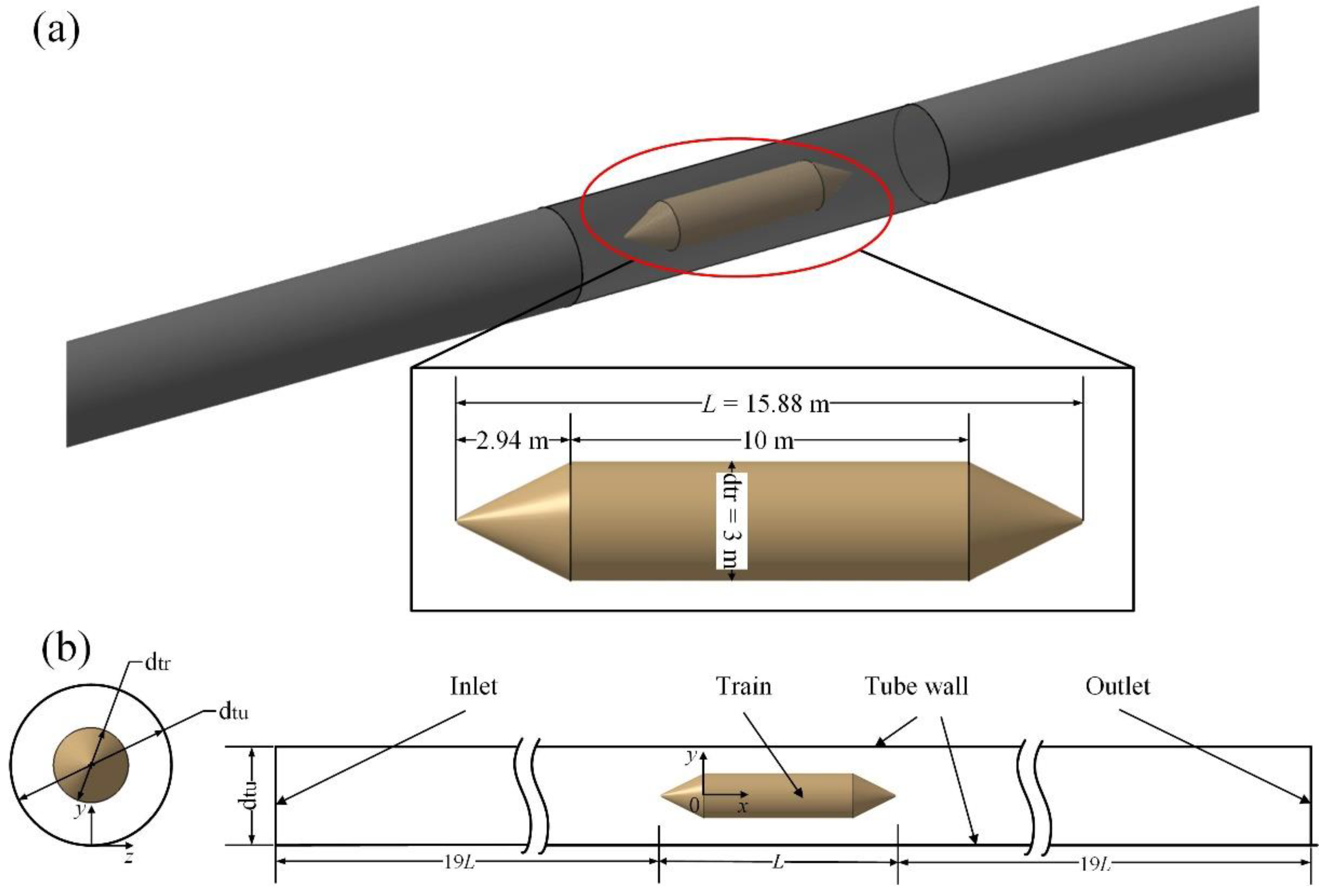
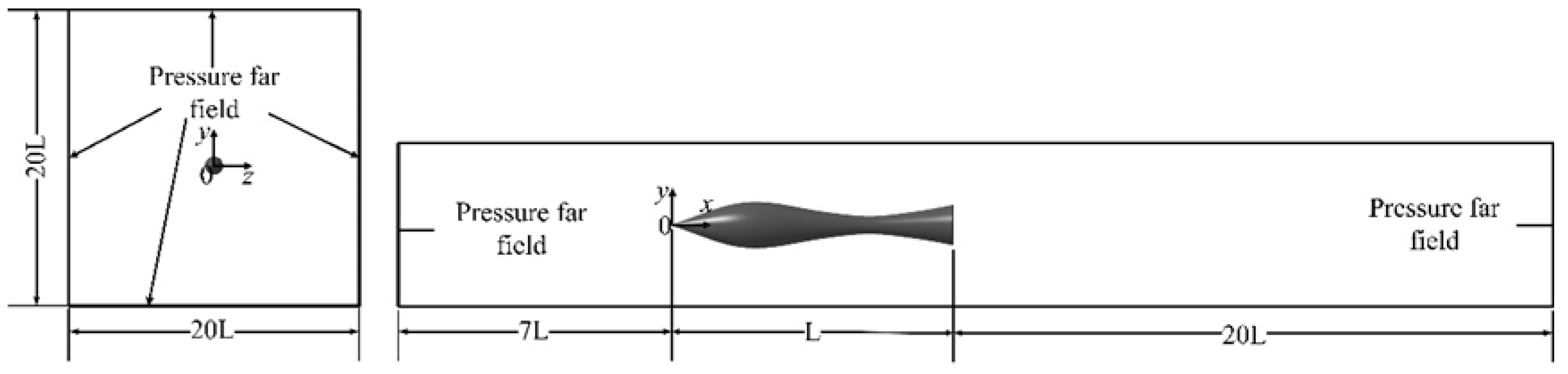
2.1. Physical Model
2.2. Numerical Method
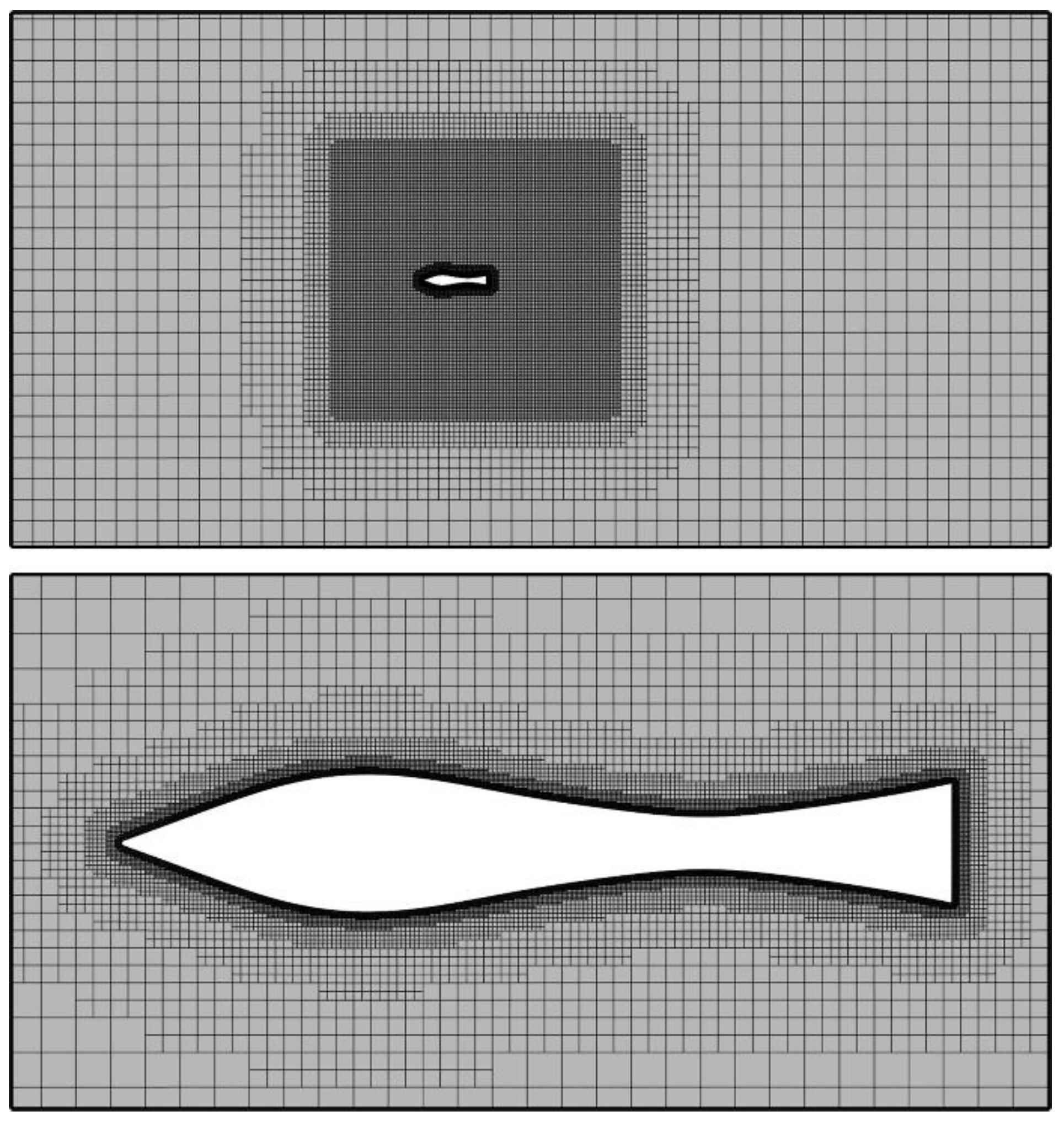
2.3. Computational Grids and Sensitivity Study
2.4. Numerical Validation
3. Result and Discussion
3.1. Comparison between the ETT and Open System
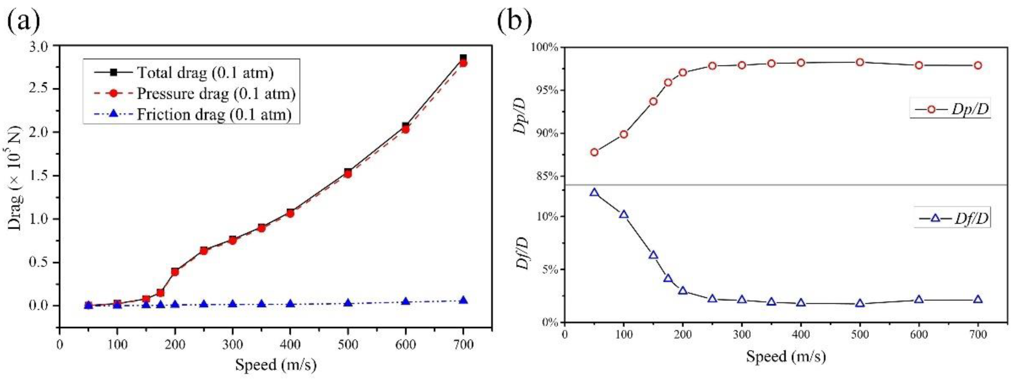
3.1.1. Drag of the Tube Train
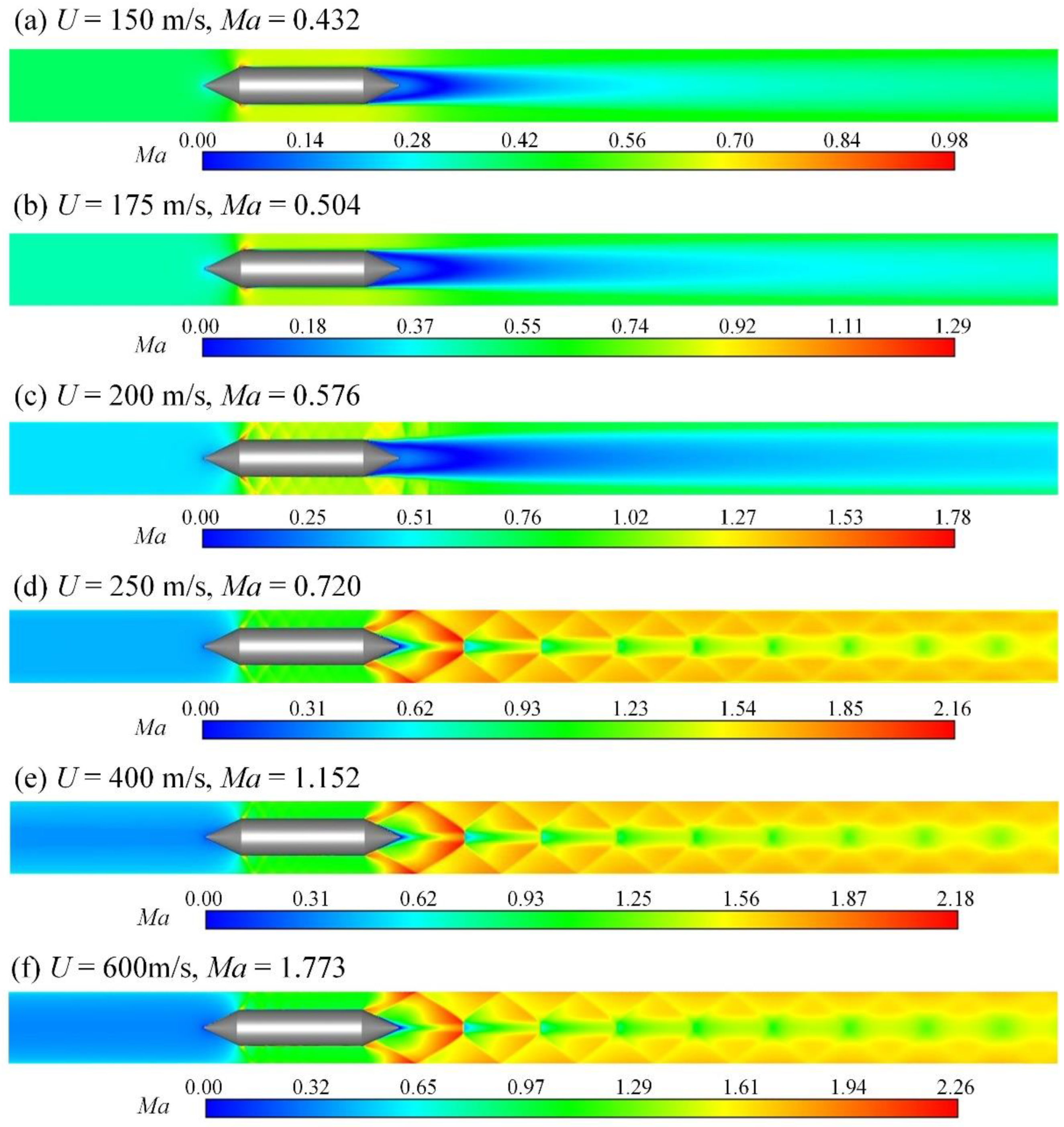
3.1.2. Flow Topology
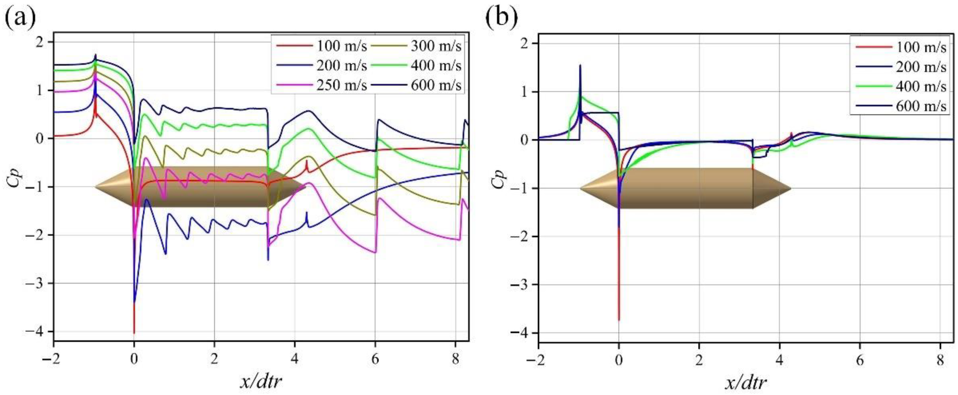
3.1.3. Pressure Distribution
3.2. The Key Aerodynamic Parameters for the ETT System
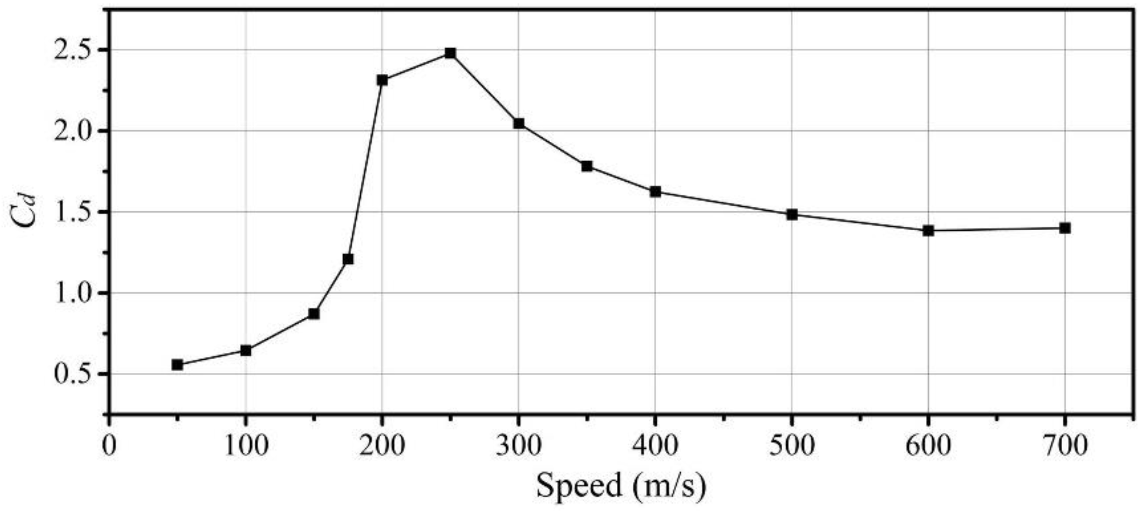
3.2.1. The Travelling Speed
3.2.2. The Ambient Pressure in the Tube
4. Conclusions
Author Contributions
Funding
Acknowledgments
Conflicts of Interest
References
- Hammitt, A.G.; Systems, T.; Beach, R. Aerodynamic analysis of tube vehicle systems. AIAA J. 1971, 10, 282–290. [Google Scholar] [CrossRef]
- Oster, D. Evacuated Tube Transport. US Patent US5950543A, 14 September 1999. [Google Scholar]
- Zhang, Y.P. Evacuated tube transportation (ETT)—A new opportunity for vacuum industry. Vacuum 2006, 43, 56–69. [Google Scholar]
- Van-Goeverden, K.; Milakis, D.; Janic, M.; Konings, R. Analysis and modelling of performances of the HL (hyperloop) transport system. Eur. Transp. Res. Rev. 2018, 10, 41. [Google Scholar] [CrossRef]
- Jiang, J.; Bai, X.; Wu, L. Design consideration of a super-high speed high temperature superconductor maglev evacuated tube transport (I). J. Mod. Transp. 2012, 20, 108–114. [Google Scholar] [CrossRef] [Green Version]
- Musk, E. Hyperloop Alpha; Space X: Hawthorne, CA, USA, 2013. [Google Scholar]
- Wong, F.T.H. Aerodynamic Design and Optimization of a Hyperloop Vehicle; The Delft University of Technology: Delft, The Netherlands, 2018. [Google Scholar]
- Shen, Z.Y. Dynamic interaction of high speed maglev train on girders and its comparison with the case in ordinary high speed railways. J. Traffic Transp. Eng. 2001, 1, 1–6. [Google Scholar]
- Giegel, J. Making hyperloop a reality: Virgin hyperloop one. Glob. Rail. Rev 2018, 24, 28–31. [Google Scholar]
- Abdelrahman, A.S.; Sayeed, J.; Youssef, M.Z. Hyperloop transportation system: Analysis, design, control, and implementation. IEEE Trans. Ind. Electron. 2018, 65, 7427–7436. [Google Scholar] [CrossRef]
- Roshan, P.; Aditya, K. Vehicle dynamics of permanent-magnet levitation based hyperloop capsules. In Proceedings of the ASME 2018 Dynamic Systems and Control Conference, Atlanta, GA, USA, 30 September–3 October 2018. DSCC2018-9130. [Google Scholar]
- Dorta, A.V.; Becker, E. The potential short-term impact of a hyperloop service between San Francisco and Los Angeles on airport competition in California. Transp. Policy 2018, 71, 45–56. [Google Scholar] [CrossRef] [Green Version]
- Kang, H.; Jin, Y.; Kwon, H.; Kim, K. A study on the aerodynamic drag of transonic vehicle in evacuated tube using computational fluid dynamics. Int. J. Aeronaut. Space Sci. 2017, 18, 614–622. [Google Scholar] [CrossRef]
- Chin, J.C. Open-source conceptual sizing models for the hyperloop passenger pod. In Proceedings of the 56th AIAA/ASCE/AHS/ASC Structures, Structural Dynamics, and Materials Conference, Kissimmee, FL, USA, 5–9 January 2015. [Google Scholar]
- Cai, Y.G.; Chen, S.S. Dynamic characteristics of magnetically levitated vehicle systems. Appl. Mech. Rev. ASME 1997, 50, 647–670. [Google Scholar] [CrossRef]
- Piechna, J. Low pressure tube transport—An alternative to ground road transport—Aerodynamic and other problems and possible solutions. Energies 2021, 14, 3766. [Google Scholar] [CrossRef]
- Edwards, L.K. High-Speed Tube Transportation. Sci. Am. 1965, 213, 30–41. Available online: https://www.jstor.org/stable/24931968 (accessed on 11 April 2019). [CrossRef]
- Axhausen, K.W. SwissMetro; Travel Survey Metadata Series; ETH Zürich: Zürich, Switzerland, 2013; Volume 42. [Google Scholar] [CrossRef]
- Bierlaire, M. The acceptance of modal innovation: In Proceedings of the Case of Swissmetro. Swiss Transport Research Conference, Ascona, Switzerland, 1–3 March 2001. [Google Scholar]
- Oster, D.; Kumada, M.; Zhang, Y.P. Evacuated tube transport technologies (ET3)tm: A maximum value global transportation network for passengers and cargo. J. Mod. Transp. 2011, 19, 42–50. [Google Scholar] [CrossRef]
- Wang, Z.T. China is developing a 4000 km/h high speed airplane train. Light Alloy. Fabric. Technol. 2018, 46, 33. [Google Scholar]
- Kim, T.K.; Kim, K.H.; Kwon, H.B. Aerodynamic characteristics of a tube train. J. Wind Eng. Ind. Aerodynam. 2011, 99, 1187–1196. [Google Scholar] [CrossRef]
- Mi, B.G.; Zhan, H.; Zhu, J. Simulation of aerodynamic drag of high-speed train in evacuated tube transportation. Chin. J. Vacuum Sci. Technol. 2013, 33, 877–882. [Google Scholar]
- Ma, J.Q.; Zhou, D.J.; Zhao, L. The approach to calculate the aerodynamic drag of maglev train in the evacuated tube. J. Mod. Transp. 2013, 21, 200–208. [Google Scholar] [CrossRef] [Green Version]
- Oh, J.S.; Kang, T.; Ham, S. Numerical analysis of aerodynamic characteristics of hyperloop system. Energies 2019, 12, 518. [Google Scholar] [CrossRef] [Green Version]
- Le, T.T.G.; Jang, K.S.; Lee, K.S.; Ryu, J. Numerical investigation of aerodynamic drag and pressure waves in hyperloop systems. Mathematics 2020, 8, 100–111. [Google Scholar] [CrossRef]
- Niu, J.Q.; Sui, Y.; Yu, Q.J. Numerical study on the impact of Mach number on the coupling effect of aerodynamic heating and aerodynamic pressure caused by a tube train. J. Wind Eng. Ind. Aerodynam. 2019, 190, 100–111. [Google Scholar] [CrossRef]
- Niu, J.Q.; Sui, Y.; Yu, Q.J. Effect of acceleration and deceleration of a capsule train running at transonic speed on the flow and heat transfer in the tube. Aerosp. Sci. Technol. 2020, 105, 105977. [Google Scholar] [CrossRef]
- Zhou, P.; Zhang, J.Y.; Li, T. Effects of blocking ratio and Mach number on aerodynamic characteristics of the evacuated tube train. Int. J. Rail Transp. 2019, 8, 27–44. [Google Scholar] [CrossRef]
- Chen, X.Y. Aerodynamic simulation of evacuated tube maglev trains with different streamlined designs. J. Mod. Transp. 2012, 20, 115–120. [Google Scholar] [CrossRef] [Green Version]
- Zhang, Y.P. Numerical simulation and analysis of aerodynamic drag on a subsonic train in evacuated tube transportation. J. Mod. Transp. 2012, 20, 44–48. [Google Scholar] [CrossRef] [Green Version]
- Wang, J.K.; Zhang, Y.; Hu, X. Aerodynamic characteristics of high-temperature superconducting maglev-evacuated tube transport. In Proceedings of the 2020th IEEE International Conference on Applied Superconductivity and Electromagnetic Devices, Tianjin, China, 16–18 October 2020. [Google Scholar]
- Debler, W.R. Fluid Mechanics Fundamentals; Prentice Hall: Englewood Cliffs, NJ, USA, 1990. [Google Scholar]
- Tong, B.G.; Kong, X.Y.; Deng, G.H. Aerodynamics; Higher Education Press: Beijing, China, 2012. [Google Scholar]
- Kantrowitz, A.; Donaldson, C.D. Preliminary Investigation of Supersonic Diffusers; National Advisory Committee for Aeronautics: Edwards, CA, USA, 1945. [Google Scholar]
- Kim, K.K. The Russian version of the transport system ‘Hyperloop’. Transp. Syst. Technol. 2018, 4, 73–91. [Google Scholar] [CrossRef]
- Bose, A.; Viswanathan, V. Mitigating the piston effect in high-speed hyperloop transportation: A study on the use of aerofoils. Energies 2021, 14, 464. [Google Scholar] [CrossRef]
- Opgenoord, M.M.; Caplan, P.C. Aerodynamic design of the hyperloop concept. AIAA J. 2018, 56, 4261–4270. [Google Scholar] [CrossRef]
- Braun, J.; Sousa, J.; Pekardan, C. Aerodynamic design and analysis of the hyperloop. AIAA J. 2017, 55, 4053–4060. [Google Scholar] [CrossRef]
- Gillani, S.A.; Panikulam, V.P.; Sadasivan, S.; Zhang, Y.P. CFD analysis of aerodynamic drag effects on vacuum tube trains. J. Appl. Fluid Mech. 2019, 12, 303–306. [Google Scholar] [CrossRef]
- Zhou, K.Y.; Ding, G.F.; Wang, Y.M.; Niu, J.Q. Aeroheating and aerodynamic performance of a transonic hyperloop pod with radial gap and axial channel: A contrastive study. J. Wind Eng. Ind. Aerodynam. 2021, 212, 104591. [Google Scholar] [CrossRef]
- Hu, X.; Deng, Z.G.; Zhang, W.H. Effect of cross passage on aerodynamic characteristics of super-high-speed evacuated tube transportation. J. Wind Eng. Ind. Aerodynam. 2021, 211, 104562. [Google Scholar] [CrossRef]
- Menter, F.R.; Kuntz, M.; Langtry, R. Ten years of industrial experience with the SST turbulence model. Turbul. Heat Mass Transf. 2003, 4, 625–632. [Google Scholar]
- Tsien, H.S. Super-aerodynamics, mechanics of rare field gases. J. Aerodynam. Sci. 1964, 13, 653–664. [Google Scholar] [CrossRef]
- Winter, K.G.; Rotta, J.C.; Smith, K.G. Studies of the Turbulent Boundary Layer on a Waisted Body of Revolution in Subsonic and Supersonic Flow. Aeronautical Research Council Reports & Memoranda. 1968. Available online: https://reports.aerade.cranfield.ac.uk/handle/1826.2/2902 (accessed on 22 June 2020).


| MESH | Coarse | Medium | Fine |
|---|---|---|---|
| Cell number (million) | 17.53 | 27.82 | 38.33 |
| Total drag_200 m/s (N) | 38,587.20 | 38,496.20 | 38,549.16 |
| Error (with fine mesh) | −0.10% | 0.14% | - |
| Total drag_400 m/s (N) | 108,249.55 | 108,076.80 | 108,189.74 |
| Error (with fine mesh) | −0.06% | 0.10% | - |
Publisher’s Note: MDPI stays neutral with regard to jurisdictional claims in published maps and institutional affiliations. |
© 2022 by the authors. Licensee MDPI, Basel, Switzerland. This article is an open access article distributed under the terms and conditions of the Creative Commons Attribution (CC BY) license (https://creativecommons.org/licenses/by/4.0/).
Share and Cite
Zhou, Z.; Xia, C.; Shan, X.; Yang, Z. Numerical Study on the Aerodynamics of the Evacuated Tube Transportation System from Subsonic to Supersonic. Energies 2022, 15, 3098. https://doi.org/10.3390/en15093098
Zhou Z, Xia C, Shan X, Yang Z. Numerical Study on the Aerodynamics of the Evacuated Tube Transportation System from Subsonic to Supersonic. Energies. 2022; 15(9):3098. https://doi.org/10.3390/en15093098
Chicago/Turabian StyleZhou, Zhiwei, Chao Xia, Xizhuang Shan, and Zhigang Yang. 2022. "Numerical Study on the Aerodynamics of the Evacuated Tube Transportation System from Subsonic to Supersonic" Energies 15, no. 9: 3098. https://doi.org/10.3390/en15093098