
On Solar Radiation Prediction for the East–Central European Region


Abstract
:1. Introduction
2. Materials and Methods
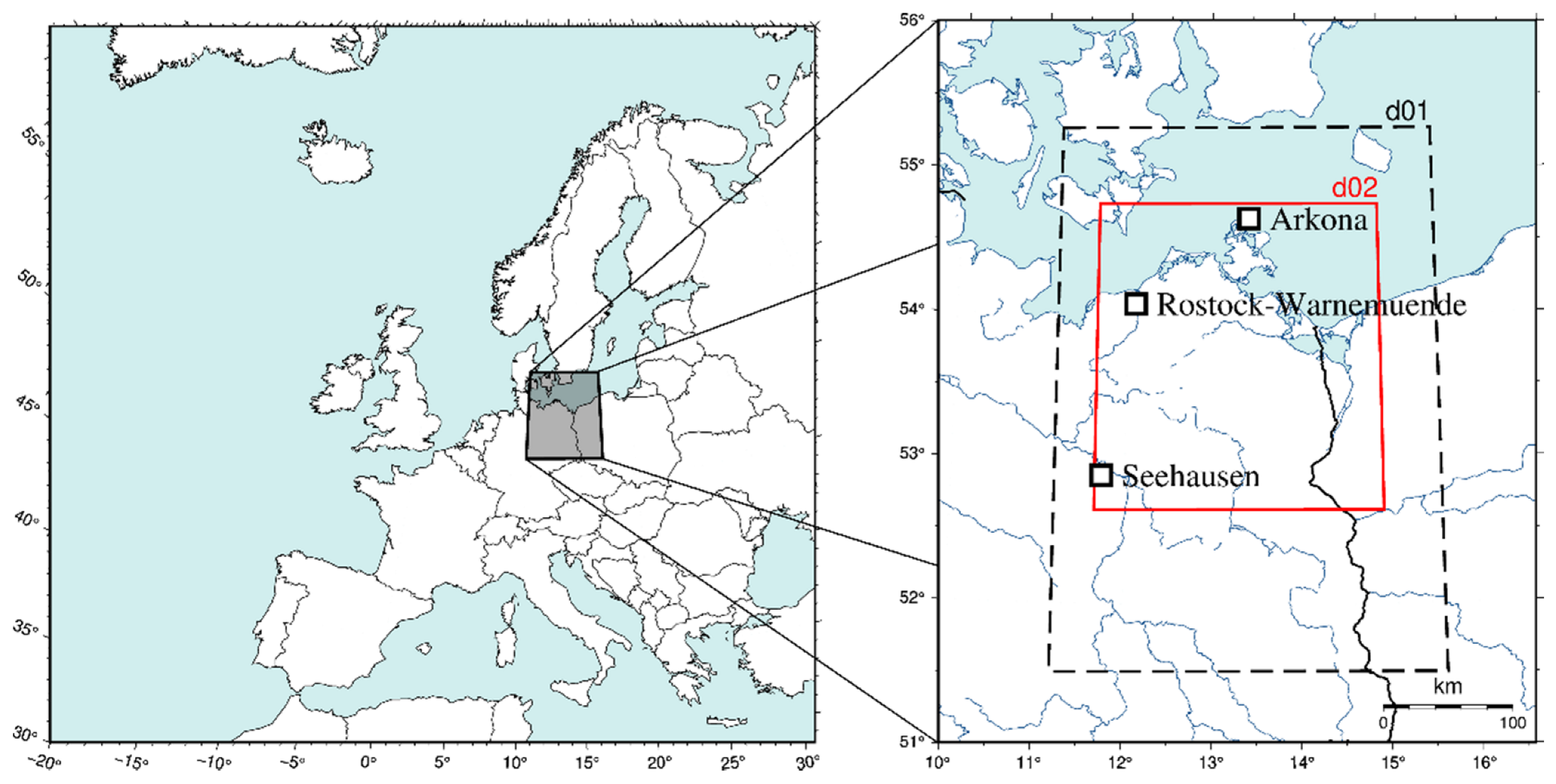
2.1. Synoptic Situations
2.2. WRF Schema
3. Results
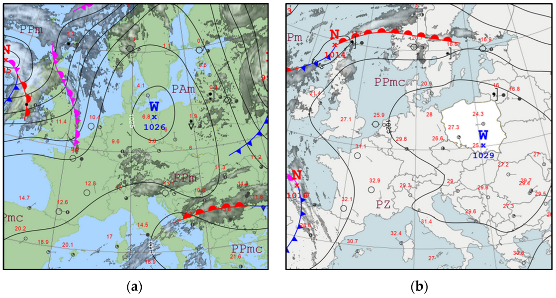
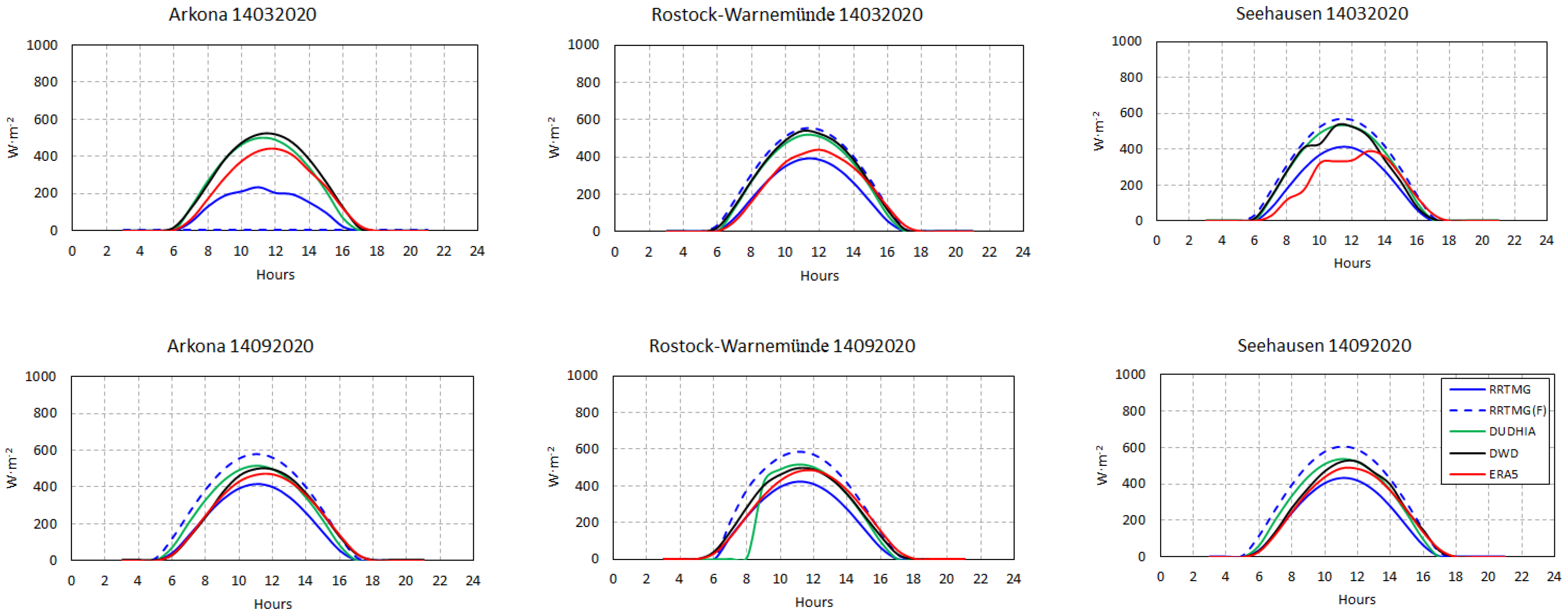
3.1. High-Pressure System
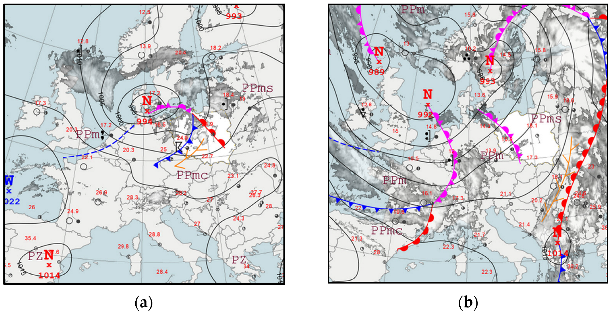
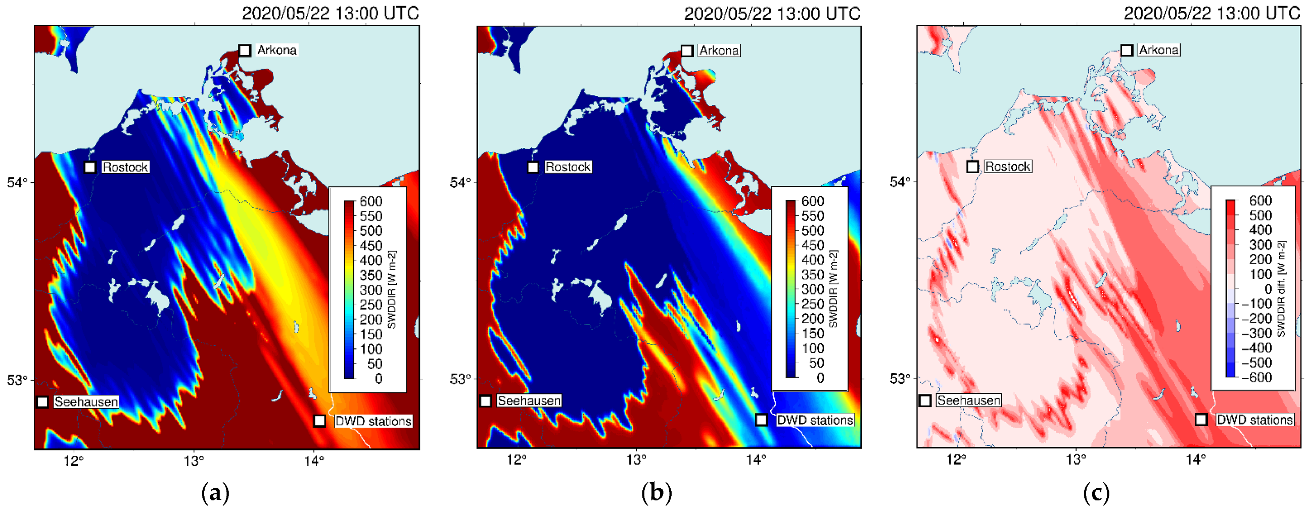
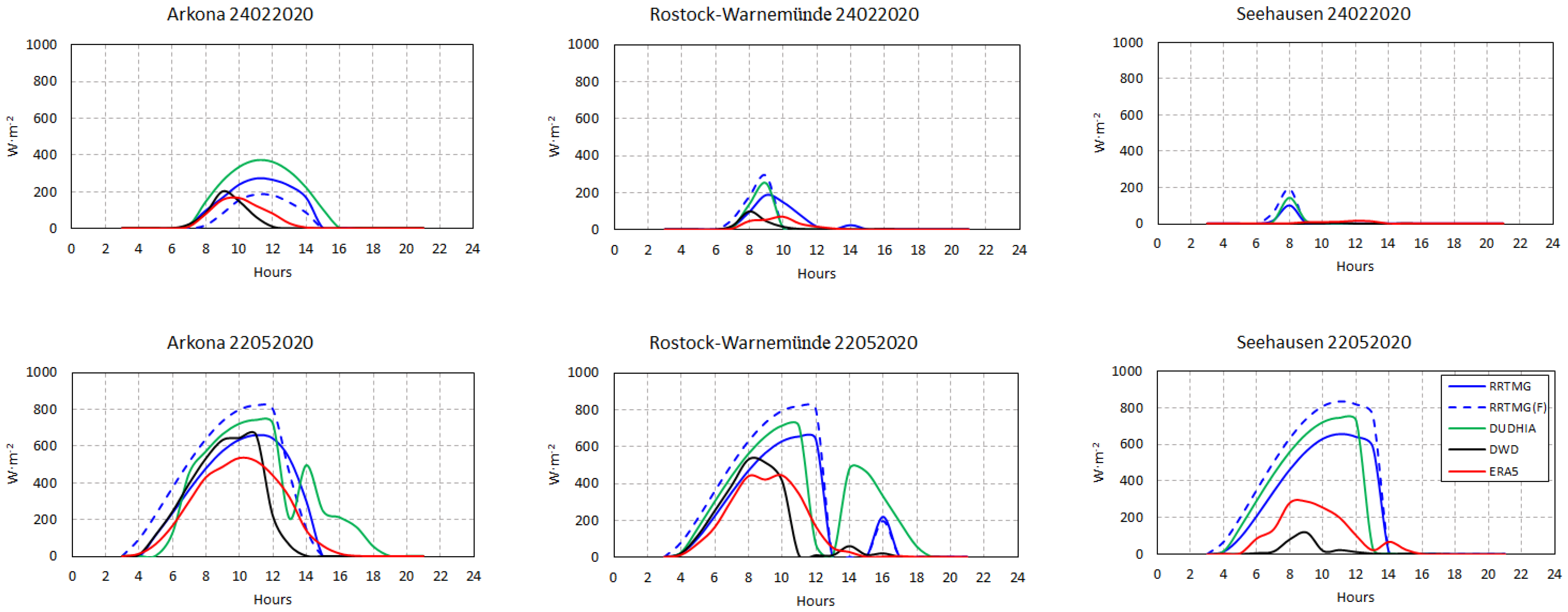
3.2. Warm Front
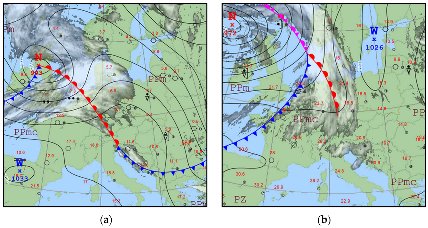
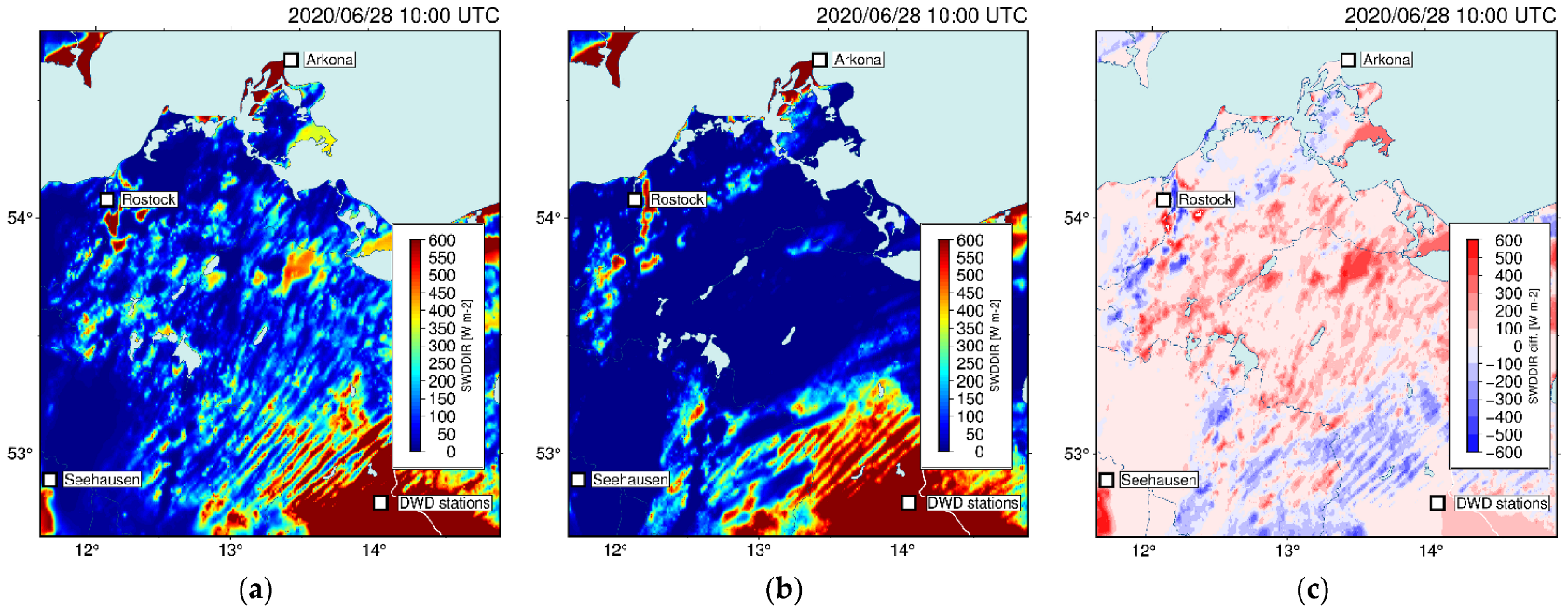
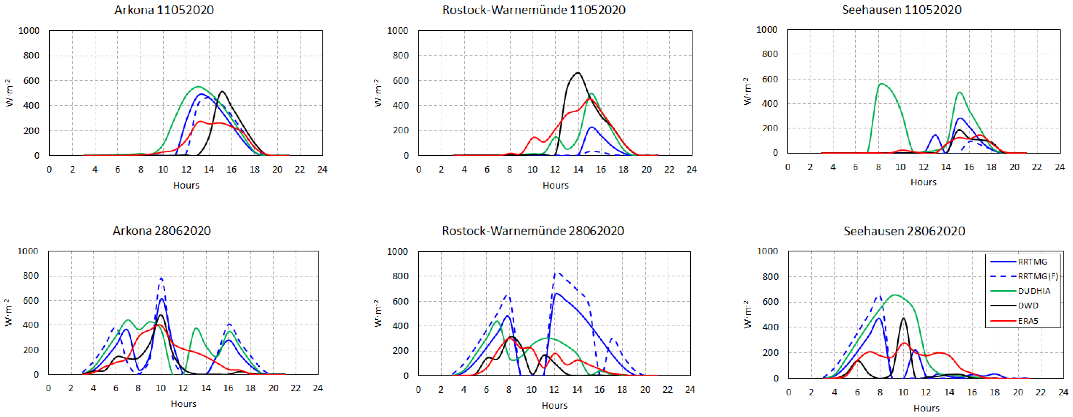
3.3. Cold Front
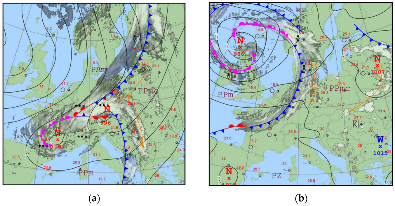
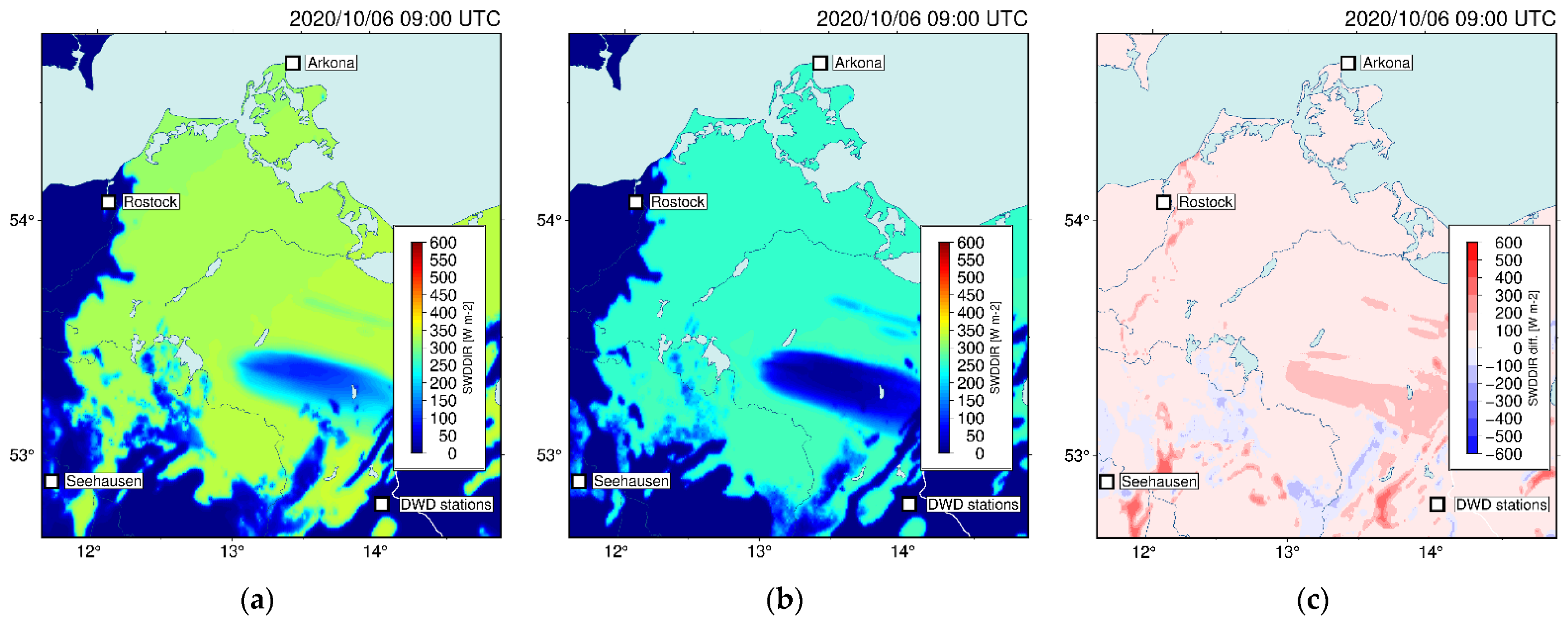
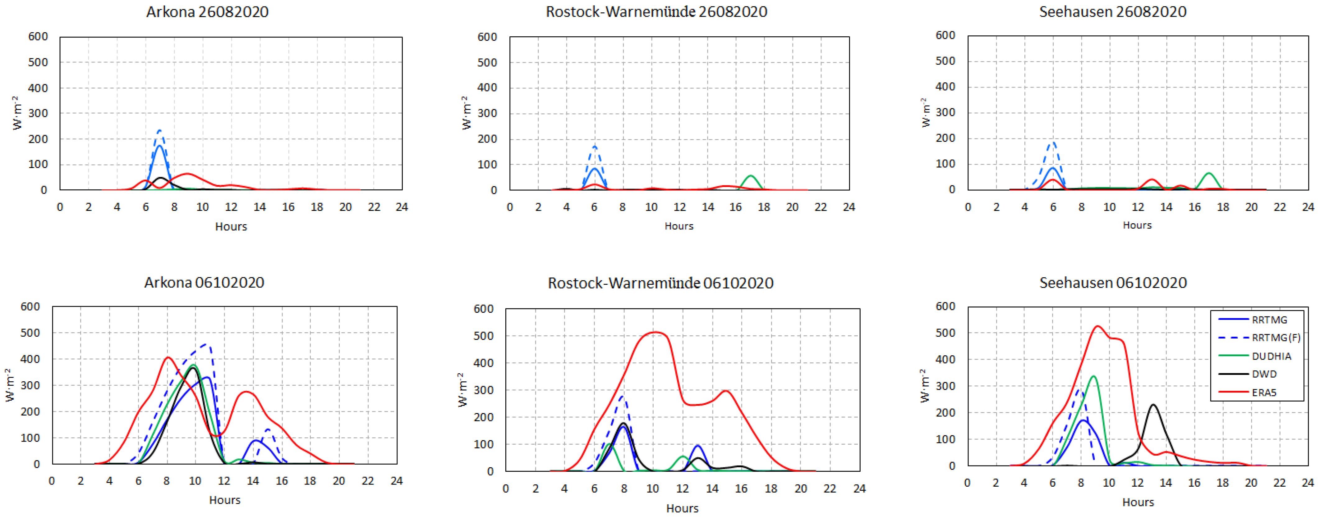
3.4. Occluded Front
4. Discussion
5. Conclusions
Author Contributions
Funding
Informed Consent Statement
Data Availability Statement
Acknowledgments
Conflicts of Interest
References
- Cross, S.; Hast, A.; Kuhi-Thalfeldt, R.; Syri, S.; Streimikiene, D.; Denina, A. Progress in renewable electricity in Northern Europe towards EU 2020 targets. Renew. Sustain. Energy Rev. 2015, 52, 1768–1780. [Google Scholar] [CrossRef]
- Perpiña Castillo, C.; Batista e Silva, F.; Lavalle, C. An assessment of the regional potential for solar power generation in EU-28. Energy Policy 2016, 88, 86–99. [Google Scholar] [CrossRef]
- Kim, J.Y.; Yun, C.Y.; Kim, C.K.; Kang, Y.H.; Kim, H.G.; Lee, S.N.; Kim, S.Y. Evaluation of WRF model-derived direct irradiance for solar thermal resource assessment over South Korea. AIP Conf. Proc. 2017, 1850, 140013. [Google Scholar] [CrossRef] [Green Version]
- Azad, E. Assessment of three types of heat pipe solar collectors. Renew. Sustain. Energy Rev. 2012, 16, 2833–2838. [Google Scholar] [CrossRef]
- Sabiha, M.A.; Saidur, R.; Mekhilef, S.; Mahian, O. Progress and latest developments of evacuated tube solar collectors. Renew. Sustain. Energy Rev. 2015, 51, 1038–1054. [Google Scholar] [CrossRef]
- Sarmiento, N.; Belmonte, S.; Dellicompagni, P.; Franco, J.; Escalante, K.; Sarmiento, J. A solar irradiation GIS as decision support tool for the Province of Salta, Argentina. Renew. Energy 2019, 132, 68–80. [Google Scholar] [CrossRef] [Green Version]
- Abu Taha, R.; Daim, T. Multi-Criteria Applications in Renewable Energy Analysis, a Literature Review. Green Energy Technol. 2013, 60, 17–30. [Google Scholar] [CrossRef]
- Mierzwiak, M.; Calka, B. Multi-Criteria Analysis for Solar Farm Location Suitability. Rep. Geod. Geoinf. 2017, 104, 20–32. [Google Scholar] [CrossRef] [Green Version]
- Mokarram, M.; Mokarram, M.J.; Khosravi, M.R.; Saber, A.; Rahideh, A. Determination of the optimal location for constructing solar photovoltaic farms based on multi-criteria decision system and Dempster–Shafer theory. Sci. Rep. 2020, 10, 8200. [Google Scholar] [CrossRef]
- Rich, P.M.; Hetrick, W.A.; Saving, S.C. Modeling Topographic Influences on Solar Radiation: A Manual for the SOLARFLUX Model; Los Alamos National Lab. (LANL): Los Alamos, NM, USA, 1995. [Google Scholar] [CrossRef] [Green Version]
- Fu, P.; Rich, P.M. A geometric solar radiation model and its applications in agriculture and forestry. In Proceedings of the Second International Conference on Geospatial Information in Agriculture and Forestry, Lake Buena Vista, FL, USA, 10–12 January 2000; pp. 357–364. [Google Scholar]
- Tovar-Pescador, J.; Pozo-Vázquez, D.; Ruiz-Arias, J.A.; Batlles, J.; López, G.; Bosch, J.L. On the use of the digital elevation model to estimate the solar radiation in areas of complex topography. Meteorol. Appl. 2006, 13, 279–287. [Google Scholar] [CrossRef] [Green Version]
- Ramirez-Vergara, J.; Bosman, L.B.; Leon-Salas, W.D.; Wollega, E. Ambient temperature and solar irradiance forecasting prediction horizon sensitivity analysis. Mach. Learn. Appl. 2021, 6, 100128. [Google Scholar] [CrossRef]
- Yang, F.; Pan, H.L.; Krueger, S.K.; Moorthi, S.; Lord, S.J. Evaluation of the NCEP Global Forecast System at the ARM SGP Site. Mon. Weather Rev. 2006, 134, 3668–3690. [Google Scholar] [CrossRef]
- Brown, A.; Milton, S.; Cullen, M.; Golding, B.; Mitchell, J.; Shelly, A. Unified Modeling and Prediction of Weather and Climate: A 25-Year Journey. Bull. Am. Meteorol. Soc. 2012, 93, 1865–1877. [Google Scholar] [CrossRef]
- Describing ECMWF’s Forecasts and Forecasting System. ECMWF. Available online: https://www.ecmwf.int/en/elibrary/17412-describing-ecmwfs-forecasts-and-forecasting-system (accessed on 16 March 2022).
- Zängl, G.; Reinert, D.; Rípodas, P.; Baldauf, M. The ICON (ICOsahedral Non-hydrostatic) modeling framework of DWD and MPI-M: Description of the non-hydrostatic dynamical core. Q. J. R. Meteorol. Soc. 2015, 141, 563–579. [Google Scholar] [CrossRef]
- Powers, J.G.; Klemp, J.B.; Skamarock, W.C.; Davis, C.A.; Dudhia, J.; Gill, D.O.; Coen, J.L.; Gochis, D.J.; Ahmadov, R.; Peckham, S.E.; et al. The Weather Research and Forecasting Model: Overview, System Efforts, and Future Directions. Bull. Am. Meteorol. Soc. 2017, 98, 1717–1737. [Google Scholar] [CrossRef]
- Weather Research and Forecasting Model. MMM: Mesoscale & Microscale Meteorology Laboratory. Available online: https://www.mmm.ucar.edu/weather-research-and-forecasting-model (accessed on 16 March 2022).
- Mandal, A.; Nykiel, G.; Strzyzewski, T.; Kochanski, A.; Wrońska, W.; Gruszczynska, M.; Figurski, M.; Mandal, A.; Nykiel, G.; Strzyzewski, T.; et al. High-resolution fire danger forecast for Poland based on the Weather Research and Forecasting Model. Int. J. Wildl. Fire 2021, 31, 149–162. [Google Scholar] [CrossRef]
- Nilo, S.T.; Cimini, D.; Di Paola, F.; Gallucci, D.; Gentile, S.; Geraldi, E.; Larosa, S.; Ricciardelli, E.; Ripepi, E.; Viggiano, M.; et al. Fog Forecast Using WRF Model Output for Solar Energy Applications. Energies 2020, 13, 6140. [Google Scholar] [CrossRef]
- Guo, Z.; Xiao, X. Wind power assessment based on a WRF wind simulation with developed power curve modeling methods. Abstr. Appl. Anal. 2014, 2014, 941648. [Google Scholar] [CrossRef]
- Tan, E.; Mentes, S.S.; Unal, E.; Unal, Y.; Efe, B.; Barutcu, B.; Onol, B.; Topcu, H.S.; Incecik, S. Short term wind energy resource prediction using WRF model for a location in western part of Turkey. J. Renew. Sustain. Energy 2021, 13, 013303. [Google Scholar] [CrossRef]
- Jimenez, P.A.; Hacker, J.P.; Dudhia, J.; Haupt, S.E.; Ruiz-Arias, J.A.; Gueymard, C.A.; Thompson, G.; Eidhammer, T.; Deng, A. WRF-SOLAR: Description and clear-sky assessment of an augmented NWP model for solar power prediction. Bull. Am. Meteorol. Soc. 2016, 97, 1249–1264. [Google Scholar] [CrossRef]
- Jiménez, P.A.; Alessandrini, S.; Haupt, S.E.; Deng, A.; Kosovic, B.; Lee, J.A.; Monache, L.D. The role of unresolved clouds on short-range global horizontal irradiance predictability. Mon. Weather Rev. 2016, 144, 3099–3107. [Google Scholar] [CrossRef]
- Lee, J.A.; Haupt, S.E.; Jiménez, P.A.; Rogers, M.A.; Miller, S.D.; McCandless, T.C. Solar irradiance nowcasting case studies near sacramento. J. Appl. Meteorol. Climatol. 2017, 56, 85–108. [Google Scholar] [CrossRef]
- Ruiz-Arias, J.A.; Dudhia, J. A simple parameterization of the short-wave aerosol optical properties for surface direct and diffuse irradiances assessment in a numerical weather model. Geosci. Model Dev. 2014, 7, 593–629. [Google Scholar] [CrossRef] [Green Version]
- Gueymard, C.; Jimenez, P. Validation of Real-Time Solar Irradiance Simulations Over Kuwait Using WRF-Solar. In Proceedings of the EuroSun 2018 Conference, Rapperswil, Switzerland, 10–13 September 2018; pp. 1–11. [Google Scholar] [CrossRef]
- Diagne, M.; David, M.; Boland, J.; Schmutz, N.; Lauret, P. ScienceDirect 2013 ISES Solar World Congress Post-processing of solar irradiance forecasts from WRF Model at Reunion Island Selection and/or peer-review under responsibility of ISES. Energy Procedia 2014, 57, 1364–1373. [Google Scholar] [CrossRef]
- Zempila, M.-M.; Giannaros, T.M.; Bais, A.; Melas, D.; Kazantzidis, A. Evaluation of WRF shortwave radiation parameterizations in predicting Global Horizontal Irradiance in Greece. Renew. Energy 2016, 86, 831–840. [Google Scholar] [CrossRef]
- Lara-Fanego, V.; Ruiz-Arias, J.A.; Pozo-Vázquez, D.; Santos-Alamillos, F.J.; Tovar-Pescador, J. Evaluation of the WRF model solar irradiance forecasts in Andalusia (southern Spain). Sol. Energy 2012, 86, 2200–2217. [Google Scholar] [CrossRef]
- Isvoranu, D.; Badescu, V. Comparison Between Measurements and WRF Numerical Simulation of Global Solar Irradiation in Romania. Ann. West Univ. Timis.-Phys. 2013, 57, 24–33. [Google Scholar] [CrossRef] [Green Version]
- Incecik, S.; Sakarya, S.; Tilev, S.; Kahraman, A.; Aksoy, B.; Caliskan, E.; Topcu, S.; Kahya, C.; Odman, M.T. Evaluation of WRF parameterizations for global horizontal irradiation forecasts: A study for Turkey. Atmosfera 2019, 32, 143–158. [Google Scholar] [CrossRef] [Green Version]
- Perez, R.; Lorenz, E.; Pelland, S.; Beauharnois, M.; Van Knowe, G.; Hemker, K.; Heinemann, D.; Remund, J.; Müller, S.C.; Traunmüller, W.; et al. Comparison of numerical weather prediction solar irradiance forecasts in the US, Canada and Europe. Sol. Energy 2013, 94, 305–326. [Google Scholar] [CrossRef]
- Kallio-Myers, V.; Riihelä, A.; Schoenach, D.; Gregow, E.; Carlund, T.; Lindfors, A.V. Comparison of irradiance forecasts from operational NWP model and satellite-based estimates over Fennoscandia. Meteorol. Appl. 2022, 29, e2051. [Google Scholar] [CrossRef]
- Beck, H.E.; Zimmermann, N.E.; McVicar, T.R.; Vergopolan, N.; Berg, A.; Wood, E.F. Present and future Köppen-Geiger climate classification maps at 1-km resolution. Sci. Data 2018, 5, 180214. [Google Scholar] [CrossRef] [Green Version]
- Schemm, S.; Sprenger, M.; Martius, O.; Wernli, H.; Zimmer, M.; Schemm, S.; Sprenger, M.; Martius, O.; Wernli, H.; Zimmer, M. Increase in the number of extremely strong fronts over Europe? A study based on ERA-Interim reanalysis (1979–2014). GeoRL 2017, 44, 553–561. [Google Scholar] [CrossRef] [Green Version]
- Catto, J.L.; Ackerley, D.; Booth, J.F.; Champion, A.J.; Colle, B.A.; Pfahl, S.; Pinto, J.G.; Quinting, J.F.; Seiler, C. The Future of Midlatitude Cyclones. Curr. Clim. Chang. Rep. 2019, 5, 407–420. [Google Scholar] [CrossRef] [Green Version]
- Catto, J.L.; Nicholls, N.; Jakob, C.; Shelton, K.L. Atmospheric fronts in current and future climates. Geophys. Res. Lett 2014, 41, 7642–7650. [Google Scholar] [CrossRef] [Green Version]
- Raible, C.C. On the relation between extremes of midlatitude cyclones and the atmospheric circulation using ERA40. Geophys. Res. Lett. 2007, 34, L07703. [Google Scholar] [CrossRef]
- IPCC. Summary for Policymakers. In Climate Change 2021: The Physical Science Basis. Contribution of Working Group I to the Sixth Assessment Report of the Intergovernmental Panel on Climate Change; Masson-Delmotte, V., Zhai, P., Pirani, A., Connors, S.L., Péan, C., Berger, S., Caud, N., Chen, Y., Goldfarb, L., Gomis, M.I., et al., Eds.; Cambridge University Press: Cambridge, UK, 2021. [Google Scholar]
- Bochenek, B.; Ustrnul, Z.; Wypych, A.; Kubacka, D. Machine Learning-Based Front Detection in Central Europe. Atmos 2021, 12, 1312. [Google Scholar] [CrossRef]
- Sykulski, P.; Bielec-Bąkowska, Z. Atmospheric fronts over Poland (2006–2015). Environ. Socio-Econ. Stud. 2017, 5, 29–39. [Google Scholar] [CrossRef] [Green Version]
- Hersbach, H.; Bell, B.; Berrisford, P.; Hirahara, S.; Horányi, A.; Muñoz-Sabater, J.; Nicolas, J.; Peubey, C.; Radu, R.; Schepers, D.; et al. The ERA5 global reanalysis. Q. J. R. Meteorol. Soc. 2020, 146, 1999–2049. [Google Scholar] [CrossRef]
- Radiation Quantities in the ECMWF Model and MARS. Available online: https://www.ecmwf.int/en/elibrary/18490-radiation-quantities-ecmwf-model-and-mars (accessed on 21 August 2021).
- DWD Climate Data Center (CDC): Hourly Station Observations of Solar Incoming (Total/Diffuse) and Longwave downward Radiation for Germany, Version Recent. Available online: https://opendata.dwd.de/climate_environment/CDC/observations_germany/climate/hourly/solar/DESCRIPTION_obsgermany_climate_hourly_solar_en.pdf (accessed on 21 August 2021).
- De Araujo, J.M.S. Performance comparison of solar radiation forecasting between wrf and lstm in Gifu, Japan. Environ. Res. Commun. 2020, 2, 045002. [Google Scholar] [CrossRef]
- Chai, T.; Draxler, R.R. Root mean square error (RMSE) or mean absolute error (MAE)?-Arguments against avoiding RMSE in the literature. Geosci. Model Dev. 2014, 7, 1247–1250. [Google Scholar] [CrossRef] [Green Version]
- Willmott, C.J.; Matsuura, K. Advantages of the mean absolute error (MAE) over the root mean square error (RMSE) in assessing average model performance. Clim. Res. 2005, 30, 79–82. [Google Scholar] [CrossRef]
- Jerzy Kondracki Fizycznogeograficzna regionalizacja Niemiec i terenów przyległych w układzie dzisiętnym. Przegląd Geogr. 1997, 69, 141–148.
- IMGW Public Data. Available online: https://danepubliczne.imgw.pl/datastore (accessed on 15 March 2022).
- National Centers for Environmental Prediction/National Weather Service/NOAA/U.S. Department of Commerce. 2015, Updated Daily. NCEP GFS 0.25 De-gree Global Forecast Grids Historical Archive. Research Data Archive at the National Center for Atmospheric Res. Available online: https://rda.ucar.edu/datasets/ds084.1/ (accessed on 21 August 2021).
- Skamarock, W.C.; Klemp, J.B. A time-split nonhydrostatic atmospheric model for weather research and forecasting applications. J. Comput. Phys. 2008, 227, 3465–3485. [Google Scholar] [CrossRef]
- Thompson, G.; Tewari, M.; Ikeda, K.; Tessendorf, S.; Weeks, C.; Otkin, J.; Kong, F. Explicitly-coupled cloud physics and radiation parameterizations and subsequent evaluation in WRF high-resolution convective forecasts. Atmos. Res. 2016, 168, 92–104. [Google Scholar] [CrossRef] [Green Version]
- Dudhia, J. Numerical Study of Convection Observed during the Winter Monsoon Experiment Using a Mesoscale Two-Dimensional Model. J. Atmos. Sci. 1989, 46, 3077–3107. [Google Scholar] [CrossRef]
- Xie, Y.; Sengupta, M.; Dudhia, J. A Fast All-sky Radiation Model for Solar applications (FARMS): Algorithm and performance evaluation. Sol. Energy 2016, 135, 435–445. [Google Scholar] [CrossRef] [Green Version]
- Cohan, D.S.; Xu, J.; Greenwald, R.; Bergin, M.H.; Chameides, W.L. Impact of atmospheric aerosol light scattering and absorption on terrestrial net primary productivity. Glob. Biogeochem. Cycles 2002, 16, 37-1–37-12. [Google Scholar] [CrossRef]
- Documentacion. Available online: https://www.ogimet.com/guia.phtml.en (accessed on 15 March 2022).


| Date | Synoptic Situation | Cloud Cover | Clouds | Dynamic Change |
|---|---|---|---|---|
| 14032020 | high pressure situation | cloudless conditions | - | low |
| 14092020 | ||||
| 11052020 | cold front | overcast/broken conditions | convective clouds | medium |
| 28062020 | ||||
| 24022020 | warm front | overcast conditions | high-, middle-, and low-level clouds | high |
| 22052020 | ||||
| 26082020 | occluded front | variable cloudiness | convective clouds | medium/high |
| 06102020 |
| Model | Chosen Configuration |
|---|---|
| Horizontal resolution | d01: 3000 (m) |
| d02: 1000 (m) | |
| Vertical resolution | 45 levels |
| Microphysics | Thompson Scheme |
| Planetary boundary layer | Mellor-Yamada Nakanishi Niino (MYNN) |
| Longwave radiation scheme | RRTMG |
| Shortwave radiation schemes | Dudhia/RRTMG |
| Land surface options | Unified Noah Land Surface Model |
| Shallow cumulus option | Deng Scheme |
| Surface layer options | Revised MM5 Scheme |
| Station | RRTMG | RRTMG(F) | Dudhia | ERA5 |
|---|---|---|---|---|
| Arkona | 0.91 | 0.54 | 0.99 | 0.99 |
| Rostock-Warnemünde | 0.99 | 0.99 | 0.97 | 0.98 |
| Seehausen | 0.99 | 0.99 | 0.99 | 0.95 |
| Station | RRTMG | RRTMG(F) | Dudhia | ERA5 |
|---|---|---|---|---|
| Arkona | 0.82 | 0.90 | 0.79 | 0.92 |
| Rostock-Warnemünde | 0.67 | 0.71 | 0.73 | 0.88 |
| Seehausen | 0.62 | 0.62 | 0.67 | 0.84 |
| Station | RRTMG | RRTMG(F) | Dudhia | ERA5 |
|---|---|---|---|---|
| Arkona | 0.64 | 0.68 | 0.45 | 0.75 |
| Rostock-Warnemünde | 0.07 | −0.02 | 0.49 | 0.84 |
| Seehausen | 0.17 | 0.62 | 0.49 | 0.60 |
| Station | RRTMG | RRTMG(F) | Dudhia | ERA5 |
|---|---|---|---|---|
| Arkona | 0.86 | 0.87 | 0.98 | 0.61 |
| Rostock-Warnemünde | 0.85 | 0.81 | 0.28 | 0.46 |
| Seehausen | −0.09 | 0.06 | −0.7 | 0.01 |
| Synoptic Situation | RMSE (W·m−2) | nRMSE (%) | MAE (W·m−2) | MBE (W·m−2) | nMBE (%) |
|---|---|---|---|---|---|
| High-pressure situation | 54.37 | 29% | 30.07 | −23.60 | −12.72% |
| Warm front | 72.23 | 118% | 36.03 | 12.44 | 20.41% |
| Cold front | 88.02 | 128% | 51.87 | 22.59 | 32.91% |
| Occluded front | 146.58 | 837% | 74.99 | 67.57 | 385.71% |
| Synoptic Situation | RMSE (W·m−2) | nRMSE (%) | MAE (W·m−2) | MBE (W·m−2) | nMBE (%) |
|---|---|---|---|---|---|
| High-pressure situation | 86.83 | 47% | 54.62 | −54.05 | −29.14% |
| Warm front | 178.98 | 294% | 77.31 | 68.36 | 112.17% |
| Cold front | 176.43 | 257% | 94.80 | 29.69 | 43.24% |
| Occluded front | 43.60 | 249% | 16.51 | 3.30 | 19.01% |
| Synoptic Situation | RMSE (W·m−2) | nRMSE (%) | MAE (W·m−2) | MBE (W·m−2) | nMBE (%) |
|---|---|---|---|---|---|
| High-pressure situation | 122.93 | 66% | 60.24 | −3.20 | −1.72% |
| Warm front | 228.32 | 375% | 103.58 | 97.65 | 160.25% |
| Cold front | 214.32 | 312% | 113.51 | 37.86 | 55.14% |
| Occluded front | 64.11 | 366% | 25.20 | 13.05 | 74.50% |
| Synoptic Situation | RMSE (W·m−2) | nRMSE (%) | MAE (W·m−2) | MBE (W·m−2) | nMBE (%) |
|---|---|---|---|---|---|
| High-pressure situation | 38.79 | 21% | 19.51 | −3.61 | −1.95% |
| Warm front | 201.59 | 331% | 98.98 | 93.87 | 154.04% |
| Cold front | 195.02 | 284% | 115.16 | 77.71 | 113.17% |
| Occluded front | 51.92 | 296% | 17.78 | 3.36 | 19.20% |
| Synoptic Situation | RRTMG | RRTMG(F) | Dudhia | ERA5 |
|---|---|---|---|---|
| High-pressure situation | 0.97 | 0.85 | 0.98 | 0.98 |
| Warm front | 0.57 | 0.54 | 0.61 | 0.87 |
| Cold front | 0.36 | 0.33 | 0.43 | 0.78 |
| Occluded front | 0.72 | 0.65 | 0.29 | 0.22 |
| Mean value | 0.65 | 0.59 | 0.58 | 0.71 |
| Station | RRTMG | RRTMG(F) | Dudhia | ERA5 |
|---|---|---|---|---|
| Arkona | 0.76 | 0.71 | 0.79 | 0.88 |
| Rostock-Warnemünde | 0.59 | 0.61 | 0.76 | 0.79 |
| Seehausen | 0.56 | 0.59 | 0.61 | 0.72 |
| Mean value | 0.64 | 0.64 | 0.72 | 0.80 |
| Data | RRTMG | RRTMG(F) | Dudhia | DWD | ERA5 |
|---|---|---|---|---|---|
| 24022020 (WF) | 1466.18 | 847.99 | 2108.85 | 519.44 | 649.97 |
| 14032020 (HPS) | 1496.27 | 0.29 | 3301.72 | 3552.78 | 2885.94 |
| 11052020 (CF) | 1985.60 | 1902.44 | 2862.07 | 1422.22 | 1501.67 |
| 22052020 (WF) | 4521.05 | 5586.32 | 5348.84 | 3541.67 | 3498.88 |
| 28062020 (CF) | 2518.94 | 2966.45 | 3613.35 | 1452.78 | 2382.94 |
| 26082020 (OF) | 189.81 | 246.44 | 22.01 | 102.78 | 274.21 |
| 14092020 (HPS) | 2769.83 | 4290.85 | 3605.88 | 3427.78 | 3366.34 |
| 06102020 (OF) | 1286.10 | 1886.60 | 1256.94 | 983.33 | 2796.83 |
| Data | RRTMG | RRTMG(F) | Dudhia | DWD | ERA5 |
|---|---|---|---|---|---|
| 24022020 (WF) | 557.83 | 552.89 | 421.13 | 180.56 | 227.38 |
| 14032020 (HPS) | 2474.33 | 3850.48 | 3436.19 | 3630.56 | 2900.63 |
| 11052020 (CF) | 475.64 | 62.44 | 1492.58 | 2355.56 | 2357.66 |
| 22052020 (WF) | 3877.19 | 5128.08 | 5201.09 | 2377.78 | 2447.81 |
| 28062020 (CF) | 3955.24 | 5204.99 | 2591.28 | 1200.00 | 1678.06 |
| 26082020 (OF) | 88.08 | 172.97 | 72.80 | 25.00 | 94.65 |
| 14092020 (HPS) | 2768.21 | 4170.89 | 3071.52 | 3491.67 | 3410.99 |
| 06102020 (OF) | 335.26 | 459.00 | 177.14 | 411.11 | 2796.83 |
| Data | RRTMG | RRTMG(F) | Dudhia | DWD | ERA5 |
|---|---|---|---|---|---|
| 24022020 (WF) | 119.75 | 256.23 | 198.79 | 16.67 | 69.31 |
| 14032020 (HPS) | 2595.91 | 3989.22 | 3553.29 | 3411.11 | 2473.49 |
| 11052020 (CF) | 753.31 | 195.63 | 2580.64 | 519.44 | 589.77 |
| 22052020 (WF) | 4197.84 | 5708.39 | 4369.90 | 311.11 | 1472.05 |
| 28062020 (CF) | 1523.99 | 1812.32 | 3546.85 | 877.78 | 1893.45 |
| 26082020 (OF) | 94.79 | 241.40 | 121.64 | 30.56 | 127.83 |
| 14092020 (HPS) | 2875.29 | 4475.20 | 3761.66 | 3627.78 | 3413.39 |
| 06102020 (OF) | 382.77 | 478.59 | 730.16 | 444.44 | 2644.67 |
Publisher’s Note: MDPI stays neutral with regard to jurisdictional claims in published maps and institutional affiliations. |
© 2022 by the authors. Licensee MDPI, Basel, Switzerland. This article is an open access article distributed under the terms and conditions of the Creative Commons Attribution (CC BY) license (https://creativecommons.org/licenses/by/4.0/).
Share and Cite
Mierzwiak, M.; Kroszczyński, K.; Araszkiewicz, A. On Solar Radiation Prediction for the East–Central European Region. Energies 2022, 15, 3153. https://doi.org/10.3390/en15093153
Mierzwiak M, Kroszczyński K, Araszkiewicz A. On Solar Radiation Prediction for the East–Central European Region. Energies. 2022; 15(9):3153. https://doi.org/10.3390/en15093153
Chicago/Turabian StyleMierzwiak, Michał, Krzysztof Kroszczyński, and Andrzej Araszkiewicz. 2022. "On Solar Radiation Prediction for the East–Central European Region" Energies 15, no. 9: 3153. https://doi.org/10.3390/en15093153
APA StyleMierzwiak, M., Kroszczyński, K., & Araszkiewicz, A. (2022). On Solar Radiation Prediction for the East–Central European Region. Energies, 15(9), 3153. https://doi.org/10.3390/en15093153