Abstract
Risk assessment and management are some of the major tasks of urban power-grid management. The growing amount of data from, e.g., prediction systems, sensors, and satellites has enabled access to numerous datasets originating from a diversity of heterogeneous data sources. While these advancements are of great importance for more accurate and trustable risk analyses, there is no guidance on selecting the best information available for power-grid risk analysis. This paper addresses this gap on the basis of existing standards in risk assessment. The key contributions of this research are twofold. First, it proposes a method for reinforcing data-related risk analysis steps. The use of this method ensures that risk analysts will methodically identify and assess the available data for informing the risk analysis key parameters. Second, it develops a method (named the three-phases method) based on metrology for selecting the best datasets according to their informative potential. The method, thus, formalizes, in a traceable and reproducible manner, the process for choosing one dataset to inform a parameter in detriment of another, which can lead to more accurate risk analyses. The method is applied to a case study of vegetation-related risk analysis in power grids, a common challenge faced by power-grid operators. The application demonstrates that a dataset originating from an initially less valued data source may be preferred to a dataset originating from a higher-ranked data source, the content of which is outdated or of too low quality. The results confirm that the method enables a dynamic optimization of dataset selection upfront of any risk analysis, supporting the application of dynamic risk analyses in real-case scenarios.
1. Introduction
Electric energy plays a crucial role in today’s society, and it is involved in almost all aspects of society’s daily routine [1]. The continuous development of the economy increases the need for energy, leading to larger-scale power systems and increasingly complex structures [2]. Furthermore, the scale and complexity of power grids are expected to increase with the growing use of renewable energy sources [3], as well as the development and implementation of smart grids [4]. As numerous businesses, public infrastructures, and private households rely on the provision of power for their daily tasks, companies in charge of the power supply need to provide energy management in a more reliable, effective, and secure way [1,5].
Power grids are exposed to a plurality of hazards such as hurricanes, earthquakes, ice storms, and floods, which can have severe consequences. The increasing frequency of extreme weather events increases the damage potential of these hazards, further highlighting the vulnerability of power systems [6]. Indeed, large-scale power outages have frequently occurred in recent years and have caused substantial economic losses [2].
Risk assessment and management have received significant attention as a tool to ensure the operational safety and reliability of power systems, becoming one of the major tasks for urban power-grid management [2]. Risk assessment of power grids generally makes use of traditional risk approaches such as reliability block diagram (RBD), fault tree analysis FTA [7], or failure mode and effect analysis [1]. Yet, the complexity of the power grids and the growing amount of data coming, e.g., from prediction systems favor the development and use of more advanced probabilistic risk-based approaches [6]. Applications of data-based approaches to power grids and energy systems range from energy management for smart buildings [8] to online fault diagnosis [9], among others (e.g., [10,11]). Risk analysis of power grids susceptible to vegetation-related hazards can adopt diverse data sources, ranging from satellite-based orthophotos to drone-based aerial images, including plane-based orthophotos or LiDAR 3D point clouds. Connected devices and access to more computing power provide additional opportunities for data-based, dynamically updated risk analyses. However, an updated and accurate risk analysis is highly dependent on the data used to inform the different parameters for calculating risk, e.g., the frequency of an event, the probability of failure, and the potential consequences of this event. Indeed, the use of different datasets for failure frequencies is an important source of uncertainty in risk analysis results [12].
In addition to better informing conventional risk analysis, multiple data sources present an opportunity for dynamic risk analysis (DRA). DRA is a concept that has mostly emerged over the last decade [13,14]. It aims to build on data availability to provide more frequent and performant risk pictures of infrastructures [15]. While DRA can benefit from the growing data source variability to diversify the possibilities of information acquisition relative to a particular parameter [4,16,17], numerous data sources may also increase data collection and processing complexity [4,18]. First, the data to process are intrinsically heterogeneous, requiring a large panel of competencies to manipulate and extract relevant information from the datasets. Second, a larger number of data sources requires selection rules for decision-making optimization, given the potential variability in the data quality. This variability can be due to, for instance, the type of considered datasets, the spatiotemporal resolution of the data, or the acquisition conditions of the datasets.
The International Standard Organization states that risk assessment should use the “best information available” and the implementation of “dynamic” approaches [19]. However, there is no guidance for applying those principles when multiple data sources are available. The present paper is a step toward closing this gap. We propose an approach for the dynamic optimization of dataset management to reduce uncertainties relative to data selection upfront of any risk calculation. The proposed method (called the three-phases method) is based on metrology concepts and metadata for characterizing the parameter-related information needed for a quantitative risk analysis (QRA).
The method focuses on three main features of the datasets impacting the quality and usability of the data for a QRA: the nature of a dataset, the discrepancies observed between the spatiotemporal attributes of the dataset and the spatiotemporal requirements for the risk analysis, and the agents and factors involved in the data management. The method integrates these three factors in a scoring system using meta-features, relying solely on metadata. The result is a ranking of the datasets, based on their informative potential relative to a baseline of “perfect information”. The method also predicts the informative potential of any new dataset originating from a list of preselected data sources using only the information available in the metadata, thus without factually analyzing the content of the datasets. Hence, the method’s application allows a continuous selection of the best candidate across all available datasets. While the implementation of the method is labor-intensive in the first iterations of the process, it can significantly increase data management efficiency in future assessments in the long term, avoiding suboptimal repetition of tasks.
The application of the method is demonstrated through a case study focusing on risk management in power grids. We focus on the role of vegetation along power lines, which represents a common source of outages in power grids, either via trees falling on the power lines or by growing under the infrastructure until grounding one phase [4,5,20,21,22].
The remainder of this paper is organized as follows: Section 2 describes the methods and concepts on which the three-phases method is founded: metadata and risk analysis/dynamic risk analysis. Section 3 presents the result, i.e., the method developed for dataset management on risk analysis. It describes the preliminary actions required for the application of the three-phases method, which is then fully detailed in the rest of the section as the main contribution of this work. Section 4 presents an application of the method to the case study. Section 5 discusses the case study results, as well as the benefits and limitations of the method, followed by conclusions in Section 6.
2. Materials and Methods—Metadata and Risk Analysis
Metadata can be defined as “data that provide information about other data” [23]. Metadata can provide structured information about a dataset without analyzing the dataset content. As highlighted by Wierling et al. [24], credible and traceable documentation of knowledge about the energy system is not possible without metadata. Despite its potential benefits for energy systems and data management optimization, the assessment of datasets through their metadata is not extensively explored in risk analysis. Indeed, there is no uniform definition of metadata to standardize the entire process of data production, processing, analysis, and use for prediction in the field of safety [25].
Data source management using its metadata in the context of risk analysis requires, at first, a clear definition of the level of analysis. In addition, it requires having a complete picture of all the datasets usable to inform the risk analysis parameters (i.e., an exhaustive description of the risk analysis parameters and a list of all the data sources usable to inform those parameters). While these two actions are common steps in risk analysis, they generally lack details that would enable an optimal dataset management. A reinforcement of those steps (“reinforcement actions”) is, thus, needed, as introduced in Section 2.2 and further detailed in Section 3.
This section presents an overview of concepts related to metadata and risk analysis. These do not constitute an exhaustive review and are limited to the description of the concepts applied in this paper.
2.1. Metadata Concepts
Metadata (i.e., “data that define and describe other data” [26]) report information concerning the structure and the content of a dataset or a service [27,28]. Metadata can be used for three main purposes: (1) content description (author, subject, etc.), (2) structural characterization (e.g., link between various parts of a resource), and (3) administrative management (access rights, file version, etc.) [29]. In addition to these features, metadata can be classified on the basis of a piece of information’s intrinsic vs. extrinsic property [30,31]. Although intrinsic properties may be assimilated to (1) content description and extrinsic properties cover, (2) structural characterization, and (3) administrative management, there is no broad consensus on the topic [32,33]. The classification and the metadata quality assessment depend, thus, on the task at hand [34], leading to new classifications if required.
Different metadata standards have been developed over the years, depending on the fields of application and the metadata’s purposes. The Metadata Standards Directory Working Group [35], a working group from the Research Data Alliance [36], has reported a community-maintained “open directory of metadata standards applicable to scientific data” [37]. An extract of this work is presented in Appendix A. This directory also reports the Dublin Core (DC), which is a generic standard developed on Semantic Web principles (or a “web of linked data”) [38,39] and managed by the Dublin Core™ Metadata Initiative, or DCMI. DCMI aims at developing and sharing best practices in the design and management of metadata. It is an open, collaborative, international, cross-disciplinary, technology-neutral, and business model-/purpose-neutral organization dedicated to supporting metadata management since the 1990s [40,41]. Dublin Core is a widely used standard, also published as an ISO standard and NISO standard [42,43,44]. It contains 15 core terms and several properties, classes, datatypes, and vocabulary encoding schemes maintained by DCMI (DC terms) [45].
The adoption of the DC standard data management for risk analysis presents several advantages, such as the following:
- many of the data sources not conventionally considered may be made available online,
- cross-disciplinary standards are critical to the comparison of heterogeneous data sources,
- the importance taken over the years and continuous increase in cloud-based technologies and web-based applications,
- the importance of facilitating the sharing of data and knowledge, the collaboration, the research and development, and the innovation adoption to third parties both in the risk community and across industries.
Furthermore, using the DC standard allows using DC-related crosswalks, facilitated by the international long-term recognition of the DC metadata standard. Crosswalks enable highlighting the nature of the overlap and gaps between different metadata standards through a table or a figure. In addition, they allow pinpointing the existence or the absence of relationships between terms existing in the respective standards [46]. Multiple examples of crosswalks linking recognized schemata can be found online, such as the one provided by the Getty Research Institute [47], the one provided by the Metadata Working Group of the Emory University [48], or the one provided by the UBC Faculty Research and Publications [49]. Non-standardized crosswalks (e.g., internal) may also be considered when discrepancies are observed between the format followed for metadata reporting in a selected file and the existing standards (e.g., due to explicit choices related to specific metadata needs, or due to a simple lack of competencies). Hence, the content from other schemas can always be linked to the Dublin Core schema.
2.2. Conventional Risk Analysis and Dynamic Risk Analysis
The concept of risk is generally related to three principal elements, as displayed in Equation (1) [50].
where s corresponds to a specific scenario, p corresponds to the probability of occurrence of this specific scenario, and c corresponds to the resulting consequences.
Risk = f(s, p, c),
Various standards adopt this definition for defining the steps of risk assessment [19,51,52]. Figure 1 presents the different steps to be followed within a risk assessment [51]. The figure also presents the placement of the proposed reinforcement actions to be described in Section 3.1, in blue and in red. Note that additional steps are identified in green in the figure: the management of datasets for informing the risk assessment. These steps consist of the method proposed in this paper, as described in Section 3.2 and Section 3.3.
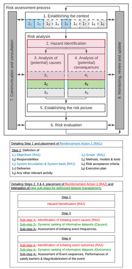
Figure 1.
Augmented risk assessment framework Z-013 [51]. The steps highlighted in blue and red are the subject of augmentation (reinforcement actions 1 and 2), and the steps 32 and 42 in green are additional steps related to the optimization of data source/dataset management.
Different sources of uncertainties may arise during a risk assessment, one of them being data processing [53]. The “level of knowledge” to represent some of these sources was added to Kaplan and Garrick’s definition (Equation (2)) by Aven and Krohn [54].
where the variable k corresponds to the level of knowledge and is added to the variables s, p, and c corresponding to scenario, probability of occurrence, and consequence, respectively.
Risk = f(s, p, c, k),
The assessment of the level of knowledge requires a proper characterization of the information pipeline, starting with the data acquisition [16,19]. The concept of “best level of information” selection, associated with the concept of “dynamicity”, can help in ensuring more efficient risk assessment and having a clear picture of the related uncertainties.
The notion of dynamicity was recently added to the principles of risk management presented within ISO 31000. Dynamic risk management approaches aim not only to update the data to consider, but also to adapt and reconsider, if necessary and on the basis of new risk evidence [55], the assumptions and models retained in previous cycles of the assessment [15,56,57,58]. As such, those techniques avoid lock-ins from initially considered conditions and process inertia by integrating, by design, the possibility to appropriately reshape the risk assessment process while minimizing the required efforts [59].
Despite the increasing number of publications and recognition of its relevance in ISO 31000:2018, DRA remains in an embryonic phase [15,60,61]. Limited research in the field hinders its implementation and the possibilities of improvements of DRA techniques. The lack of a systematic approach for identifying available data, as well as characterizing and managing data sources, also poses a challenge for the adoption of DRA, as it is a data-driven method. The method proposed in this paper intends to address this gap through the reinforcement actions detailed in Section 3.1 and the addition of two steps, presented in Section 3.2 and Section 3.3.
3. Results—Dataset Management Method for Dynamic Risk Analysis of Large-Scale Infrastructures
This section presents the resulting method developed for dataset management. It starts by describing the reinforcement steps required to apply the three-phases method. In Section 3.1, the main building blocks of the method are presented in Section 3.2, followed by the detailed description of the method elements in Section 3.3.
3.1. Risk Analysis Framework Reinforcement: Level of Analysis and Dataset Characterization
This subsection first details to which extent information should be characterized to enable a standard risk assessment. It then presents two reinforcement actions (RA1 and RA2) applied to existing steps of a standard risk assessment (Figure 1), namely, establishing the context (sub-steps 11, 12, 15) (RA1) and hazard identification (step 2), analysis of potential initiating event (sub-step 31), and analysis of potential consequences (sub-step 41) (RA2). The reinforcement of these steps is necessary for applying the proposed method for dataset selection (Section 3.2 and Section 3.3).
3.1.1. Information Characterization Requirements
Considering that the numerical values used within a QRA are all directly or indirectly based on measurements, best practices applied in metrology (i.e., the “science of measurement and its application” [62]) can be adopted as a reference. The measurement process in metrology is defined as “a set of operations to determine the value of a quantity” [63]. Its design represents a critical phase and consists, from a high-level point of view, in answering the following questions to execute a measurement adequately:
- Which quantity shall be measured?
- What are the required quality indicators (e.g., accuracy, precision, (see Figure 2))?
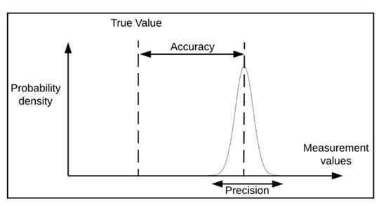 Figure 2. Accuracy–precision distinction. Illustration of the distinction between the concepts of accuracy (closeness of agreement between a measured value and a sought out true value) and precision (closeness of agreement between measured values obtained by replicate measurements on the same or similar objects under specified conditions) [62].
 - Which measurement methods shall be used?
- Which equipment shall be used?
- Which software shall be used?
- Who is going to execute the measurement?
- What are the ambient conditions and influencing quantities affecting the measurement process?
Providing the described level of detail is critical for the validity of a measurement result, and to improve the traceability of a measurement. This is particularly relevant for risk assessment and recalls the paramount importance of a proper context characterization. Indeed, answering the question “Which quantity shall be measured?” requires first an adequate identification of the information that is sought out. This action should be executed within step (1) of the risk assessment (Figure 1) (“establishing the context”), as part of the global definition of the problem to address.
Three main points among those reported in the context establishment of the NORSOK Z-013 standard [51] need to be defined to adequately characterize the information one should look for:
- The objectives (defining the objective functions and indicating which type of information should be chosen),
- The scope (characterizing to which extent this information needs to be researched),
- The system boundaries (characterizing under which considerations and within which system delimitations the data need to be sought out).
3.1.2. Reinforcement Actions: Level of Analysis and Available Data Sources
The implementation of risk analyses is, in practice, strongly constrained by the availability of needed resources [64,65]. Hence, the adequate level of analysis is a tradeoff decision between stakeholder expectations and analytical possibilities [66,67]. Figure 3 illustrates the nature of the tradeoff to be found when defining the optimal level of analysis. The optimal analysis level can be considered as the level of convergence between a top-down and a bottom-up process. The top-down process consists of the progressive detailing of a global ambition associated with a resource budget allocation. The bottom-up process consists of progressively aggregating and restoring required information most efficiently while reducing information loss [68]. The dotted line in Figure 3 can be read as the level of convergence; it can be scrolled up or down depending on objectives and conditions. Note that no budget would enable a microscopic analysis of a large and complex system, and some level of abstraction is inevitable. On the other hand, no analysis can be limited to a high-level identification of risk-related objectives, and some level of details will always be required for meaningful decision making.
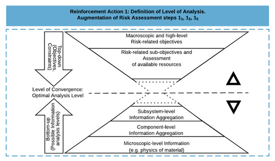
Figure 3.
Level of analysis of a risk assessment defined as tradeoff decision between stakeholder expectations and analytical possibilities.
The definition of the optimal level of analysis is related to steps 11, 12, and 15 of the risk assessment method, namely, definition of objectives, definition of the scope, and definition of system boundaries and systems basis (Figure 1). Defining the level of convergence (reinforcement action 1) supports identifying the most relevant system, subsystem, assembly, subassembly, or component on which a risk assessment shall be executed. Following this identification, the next phase consists of building on the following steps commonly applied in risk assessment [69], augmented with reinforcement action 2, as presented in Figure 4:
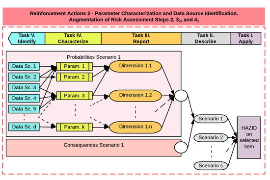
Figure 4.
Identification of parameter characterization requirements and data sources potentially exploitable for the risk analysis.
- Task (I): applying a hazard identification (HAZID), i.e., identifying all relevant hazards and hazardous events,
- Task (II): describing the relevant accident scenarios,
- Task (III): reporting all dimensions to be considered for the hazardous events addressed in each scenario, from both a probability and a consequence perspective,
- Task (IV): identifying and characterizing all relevant parameters per reported dimension,
- Task (V): identifying all the data sources providing, to any extent, information to those parameters on the basis of experience, expertise, and further benchmarks.
Reinforcement action 2 consists, thus, of preselecting a list of data sources to inform different parameters which, in turn, inform different dimensions needed for quantifying the probability of occurrence and the consequences of a specific scenario. The list of preselected data sources should be completed by looking at all the accessible data sources and determining if those can provide (to any extent possible) knowledge about the needed parameters. For traceability, the preprocessing tasks enabling one to link a data source to a parameter shall also be reported.
The characterization of the parameters (Task IV) is a crucial step. It starts by reporting attributes relevant in any measurement process, i.e., the unit, the optimal resolution, and the range.
At this stage, considering that suboptimal resolution may often be faced, it is also strategical to define acceptable subcategories of information as second-best options to enable a semiquantitative evaluation when no other possibilities exist.
Risk analysis should ideally be site-specific [13,58] and performed in real time to avoid the possibility of building on outdated data and outdated considerations [70]. Therefore, risk analyses are time- and location-sensitive, and any spatiotemporal divergence between the site to be analyzed and the data that are considered will impact the results. Thus, the following questions should also be answered for characterizing the risk parameters:
- How location-sensitive is the parameter under review?
- What is the spatial extrapolation potential, i.e., the capacity, given data provided for a particular parameter in a delimited geographical area, to estimate values for that specific parameter in the surrounding of the initially considered area?
- How quickly does the parameter under review usually change over time?
- What is the relevant time changing rate?
- How long would it take before the dataset considered for the parameter under review to be outdated?
Depending on the scope of the risk assessment being performed, an applicable spatial scale may be the following (in square meters): “not applicable (NA), individual or <100”, “<101”, “<102”, “<103”, “≥103”. Similarly, a timescale could be reported as “hours”, “days”, “weeks”, “months”, “years”, “decades”, or “constant” (i.e., no change over the lifetime of the site).
In summary, a parameter pa can be characterized through the vector
where, within a pre-defined scope, Rspa corresponds to the optimal resolution of the parameter pa based on the chosen unit, SLIpa corresponds to the sublevel of information of the parameter pa acceptable for semiquantitative evaluations, Rapa corresponds to the range of values taken by the parameter pa, SEPpa corresponds to the spatial extrapolation potential of the parameter pa, and TSpa corresponds to the temporal sensitivity of the parameter pa.
Thus, the implementation of the actions reported up to step 31 in Figure 1, reinforced with the reinforcement actions 1 and 2, allows obtaining a preselection of all potentially relevant data sources. Additionally, it enables one to precisely list the attributes usable for a quality assessment of the information provided by a dataset in terms of risk quantification.
3.2. Dataset Management: Three-Phases Method Overview
Data quality assessment has a long research history [71] and is usually executed by comparing the value of specified data quality indicators to preliminary defined reference values. The quality of the information can be assessed using various dimensions, such as accuracy, precision, coverage, completeness, timeliness, reliability, trustworthiness, traceability, comparability, costs, and metadata [72,73,74,75,76,77,78,79]. Section 3.2.1 discusses the most relevant dimensions for risk analysis and shows how those can be characterized using the terms defined in the Dublin Core standard. This is then used as the foundation for the proposed data management method, described in Section 3.2.2.
3.2.1. Dataset Characterization for Risk Analysis
Efficient dataset management for risk analysis relies on the characterization of three main features, as described below: nature of the dataset, site/time specifications of the dataset, and agents and factors influencing data management.
- (i)
- Nature of the datasetThe technologies used to capture data determine which type of file will be generated. This directly impacts the obtainable performance in terms of resolution, range coverage percentage (how much of the predefined range can be covered), precision, and accuracy. For instance, the best spatial resolution available via commercial satellite images is much lower than that provided by LiDAR point clouds (30 cm vs. a few millimeters) [80,81,82]. Furthermore, satellite images are mainly used to provide 2D information, while LiDAR point clouds are usually used to obtain 3D insights.
- (ii)
- Spatiotemporal characterization of dataFigure 5 illustrates information provided for a unique and generic parameter, at three different resolutions, at three points in time (t − 2, t − 1, and t), for a specific area of interest (AoI). While the most recent dataset with the highest resolution would be ideal, datasets are most often incomplete. Therefore, one may face situations where the highest spatial resolution is only available within an older dataset (e.g., t − 2 here), making datasets with coarser spatial resolution the only up-to-date option [83]. Additionally, one may also face a total absence of information in some regions (represented by the black region).
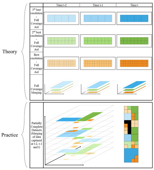 Figure 5. Differences between theory and practice in the spatiotemporal characterization of a generic parameter in a predefined area of interest (AoI). Incomplete datasets encountered in practice lead to the dilemma of sometimes having to choose between resolution and timeliness to inform the chosen parameter. Additionally, some regions may show total absence of information (black region in merged 2D view of the AoI at the bottom right of the image), which is particularly problematic for a risk assessment to be executed in that area.The management of incomplete datasets is an important task to be performed for most of the parameters involved in a risk analysis. This highlights the importance of adequately addressing the spatiotemporal characterization of the information provided by a dataset, and including it as a comparison and evaluation criterion.
 - (iii)
- Agents and factors influencing data managementThe value of information available in a dataset strongly depends on the competencies of the actors involved in the various steps of the data management (i.e., data capture, data transmission, data storage, data pre-processing, information processing, results transmission) [16,71]. The trust to be given to the information provided by a dataset is, thus, strongly influenced by, e.g., the standards and protocols followed when managing the data, the authority, and legitimacy of the actors involved [39,84].Identifying the “trust” level, the spatiotemporal features and the nature of the dataset are, thus, essential for the characterization of the datasets to be used for risk assessment. These three features are the foundation for the data management in the three-phases method. Note that the implementation of reinforcement actions 1 and 2 as previously described is required to apply the method (Figure 6).
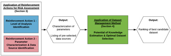 Figure 6. Logic of steps for applying the data management method. The reinforcement actions applied on common risk assessment frameworks provide the parameter characteristics required for a QRA, as well as a list of data sources that can be used to inform those.
3.2.2. Three-Phases Method—Logic Description
The Dublin Core standard presented in Section 2.1 is used as a foundation to exploit the metadata in the three-phases method. We start by only selecting the terms that are relevant for risk assessment purposes, i.e., those related to the three features defined in Section 3.2.1. We then regroup the terms into three classes by following a similar logic: (1) file (nature of the dataset), (2) scene (site-/time-specifications of the dataset), and (3) objectives/author/circumstances (agents and factors influencing data management). Table A2, Table A3 and Table A4 in Appendix B detail this recategorization, together with the respective definition of each of the selected terms [45].
The terms categorized in the first class ((1) file) report the nature of the file. They are used to characterize the default maximum potential of knowledge (DMPK) that a specific data source can provide, based on the technological possibilities of the technique used to generate the dataset (e.g., satellite-based orthophoto, LiDAR-based point cloud).
The terms categorized in the second class ((2) scene) report the spatiotemporal properties of the file. This class can be divided into two subclasses: (2a) spatial and (2b) temporal. The use of information provided in class (2) scene enables one to calculate a first degradation factor (DF1, composed of DF1a and DF1b, relative to spatial and temporal information, respectively) on the basis of the difference in nature between the spatiotemporal requirements of the site to be analyzed and the spatiotemporal properties of the considered dataset.
The terms categorized in the third class ((3) objectives/author/circumstances) report contextual information. They enable calculating a second degradation factor (DF2), characterizing the level of trust one assigns to the analyzed dataset. In opposition to the first degradation factor, the second degradation factor calculation can be considered as a more dynamic and subjective task, as the trust level is strongly influenced by the stakeholders supervising the risk analysis [85]. For instance, understanding a problem and the knowledge of the mentioned actors/standards could be very different between two distinct teams [86], a standard may become outdated and withdrawn after some time, etc.
Figure 7 illustrates the sequencing of the phases required to calculate an assessed dataset’s informative potential (i.e., potential of knowledge).
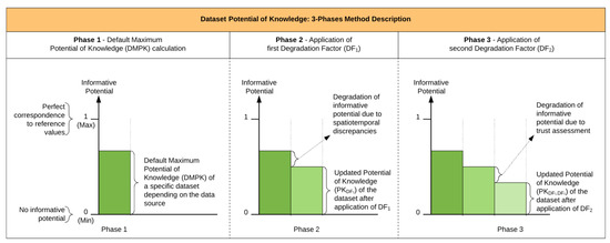
Figure 7.
Three-phases method description. The figure shows the progressive degradation in the assessment of a dataset’s informative potential when compared to the originally required level of information.
The notions of “degradation factors” have been chosen because divergences observable via the analysis of properties relative to terms in class (2) scene and (3) objectives/author/circumstances can only neutrally or negatively impact the maximum performances of the knowledge acquired via the analysis of properties relative to terms in class (1) file.
The analytical order of the phases aims to optimize future data processing: the spatial overlap is assessed before analyzing the temporal properties to automatically discard non-overlapping datasets. Furthermore, one may still decide to valorize the analysis of properties relative to terms present in classes (1) file and (2) scene, despite a lack of qualifications leading to an absence of trust-related quality check. Including trust-related quality checks in the final calculation may, thus, have to be appreciated on a case-by-case study of the problems, justifying a final position for this task in the method.
Table 1 presents the assumptions considered during the development of the method, followed by a detailed description of each of the phases in the next subsection.

Table 1.
List of assumptions made for the development of the presented method.
3.3. Quantitative Elements of the Three-Phases Method
The three-phases method identifies and characterizes multiple data source/dataset properties through a number of classes and respective boundaries. The characterization of these classes is based on the authors’ experience with data management for risk analysis. Those choices are valid from a generic perspective to the best of our knowledge. However, the method offers the flexibility for this information to be adapted to the context in which the method will be applied. The values shall, thus, be seen as an indication instead of a static and rigid formalization. The implications of those choices are further discussed in Section 5.
3.3.1. Phase 1: Default Maximum Potential of Knowledge (DMPK)—Calculation
The evaluation approach of class (1) file consists of the calculation of the DMPK, which is assessed per data source sr and per parameter pa (i.e., DMPKsr,pa). The DMPKsr,pa is a function of four properties identified on the basis of common data quality assessment criteria [71] to estimate how well preselected data sources can inform a parameter. The DMPK can be calculated through a normalized weighted sum as in Equation (3).
where the variables are defined as follows:
- DMPKsr,pa: default maximum potential of knowledge per data source sr and per parameter pa,
- LoIsr,pa: the level of information for source sr and parameter pa,
- RaCsr,pa: the range coverage for source sr and parameter pa,
- Prsr,pa: the precision for source sr and parameter pa,
- Acsr,pa: the accuracy for source sr and parameter pa,
- xLoI, xRaC, xPr, xAc: weights given by stakeholders to the level of information, the range coverage, the precision, and the accuracy of the data, respectively.
The weights give stakeholders the possibility to manage the importance given to meta-parameters as wished. For simplicity, a naïve approach setting those weights to 1 is applied for the rest of the present paper [87].
The use of the DMPK enables a first ranking of data sources based on their capacity to inform a specific parameter. Thereby, any new dataset ds originating from one of the reported data sources will automatically be given a DMPK score enabling an estimation of its a priori value for risk analysis.
Calculating the DMPK allows the stakeholders to identify the parameter characterization benefiting the most from data coming from a specific data source by assessing the DMPK scores for a unique source, and identify which dataset shall be used to inform a particular parameter depending on the origin of the different sets.
The four properties used for the DMPK calculation are described below.
Property 1.1.
Category of Obtainable Level of Information.
The obtainable level of information (LoIsr,pa) required per parameter is based on the reachable resolution provided by the data source (Table 2), adapted from the classification of [62].
Table 2.
LoIsr,pa—obtainable level of information.
- Precise measurement, enabling to reach the expected resolution and, therefore, unlocking a potential full quantification,
- Acceptable sublevel of information, enabling a semiquantitative evaluation,
- Qualitative information (e.g., yes/no; +/−; shift of tendancy (e.g., mean)),
- None.
Property 1.2.
Range Coverage Potential.
The range coverage potential (RaCsr,pa) concerns the completeness of a data source (i.e., the capacity for a data source to cover “all required parts of an entity’s description” [88]). It can be used for characterizing a candidate dataset by answering the question “How much of the predefined range can be covered?” (Table 3).
Table 3.
RaCsr,pa—range coverage potential.
Property 1.3.
Precision Estimation.
The precision meta-feature (Prsr,pa) indicates the precision of a data source, characterized through expert knowledge. The purpose is to evaluate, on the basis of experience, if the data source enables to systematically come to identical conclusions when assessing datasets acquired under repeatability conditions. This assessment is made by answering the question “Would an expert always come to the same conclusion when assessing datasets acquired under repeatability conditions?” (Table 4).
Table 4.
Prsr,pa—precision.
Property 1.4.
Accuracy Estimation.
The accuracy of a data source (Acsr,pa) is estimated through a classification built on expert knowledge. The purpose is to assess, on the basis of experience, the potential for the acquisition method to provide measurements centered around the true value. This assessment is, thus, made by answering the question “Does the method usually enable to provide conclusions centered around the true value?” (Table 5).
Table 5.
Acsr,pa—accuracy.
3.3.2. Phase 2: First Degradation Factor (DF1)—Calculation and Application
The evaluation approach of class (2) scene is performed by calculating the first degradation factor DF1. To calculate DF1, we start by applying a subcategorization of the terms reported in Table A3, Appendix B. At this stage, one mainly looks for four types of information relative to the parameters pa evaluated in each considered dataset ds:
- Where the data were acquired (acquisition area (AAds,pa)),
- With which spatial resolution the data were acquired (spatial resolution (SReds,pa)),
- When the recording of the data was initiated (Datemin,ds,pa) and, in case several recordings of them area are available, when the recording of the data was stopped (Datemax,ds,pa) (i.e., temporal range (TRads,pa)),
- With which temporal resolution the data were acquired (temporal resolution (TReds,pa)).
Therefore, assuming adequately registered metadata, one can decide to only focus on the terms 2.2a “spatial” and 2.2-b “temporal” in Table A3, Appendix B, for which detailing via subcategories (acquisition area, spatial resolution, temporal range, temporal resolution) can be used to report the required information. The rest of the terms in Table A3, Appendix B are considered redundant and potentially suboptimal for a spatiotemporal characterization relevant to risk analysis.
For simplicity, we further assume that no missing information is reported regarding the terms “spatial” and “temporal”. In addition, inspired by [79] and as further detailed where required in the following, we also suggest using additional dataset quality indicators. Although those are not initially reported in the DC standard, this information can automatically be added to existing metadata. In particular, we suggest inferring new spatiotemporal related terms using additional generic data quality measures, such as the number of missing values, non-expected records, or invalid records. This choice is further discussed in Section 5.
The global DF1 can be calculated for any dataset ds and related parameter pa as
where the variables are defined as follows:
- DF1,ds,pa: first degradation factor calculated per candidate dataset ds and per parameter pa,
- DF1a,ds,pa: first degradation factor due to spatial properties, calculated per candidate dataset ds and per parameter pa,
- DF1b,ds,pa: first degradation factor due to temporal properties, calculated per candidate dataset ds and per parameter pa.
The calculation detailing of DF1a,ds,pa is presented in Section 3.3.2.1, and that of DF1b,ds,pa is presented in Section 3.3.2.2.
An updated score can be given to the potential of knowledge (PK) for any dataset ds and related parameter pa as in Equation (5).
where the variables are defined as follows:
- PKDF1,ds,pa: updated potential of knowledge of the dataset ds and related parameter pa after applying the first degradation factor,
- DMPKsr,pa: default maximum potential of knowledge per data source sr and per parameter pa,
- DF1,ds,pa: first degradation factor calculated per candidate dataset ds and per parameter pa.
The calculation of the updated potential of knowledge (PKDF1,ds,pa) enables reconsideration and potentially reorganizing the ranking originally provided at the end of phase 1.
3.3.2.1. DF1a—First Degradation Factor Due to Spatial Properties
DF1a, the first element to be determined for setting up the global DF, is calculated per candidate dataset ds and per parameter pa (i.e., DF1a,ds,pa). We consider five properties, which are further detailed below, to estimate the quality of a dataset with regard to its spatial characteristics. Those are used to determine the form of DF1a through a normalized weighted sum as
where the variables are defined as follows:
- DF1a,ds,pa: first degradation factor due to spatial properties, calculated per candidate dataset ds and per parameter pa,
- SCds,pa: spatial coverage of candidate dataset ds per parameter pa,
- SReds,pa: spatial resolution of candidate dataset ds per parameter pa,
- SDeds,pa: spatial density of candidate dataset ds per parameter pa,
- SDids,pa: spatial distribution of candidate dataset ds per parameter pa,
- SNds,pa: spatial noise of candidate dataset ds per parameter pa,
- xSC, xSRe, xSDe, xSDi, xSN: weights given by stakeholders to the spatial coverage, spatial resolution, spatial density, spatial distribution, and spatial noise of the data, respectively.
The weights give stakeholders the possibility to manage the importance given to meta-parameters as wished. For simplicity, a naïve approach setting those weights to 1 is applied for the rest of the present paper [87].
Given a list of predefined thresholds and the score obtained for DF1a,ds,pa, one can automatically assess whether further processing a dataset under review is meaningful; further analysis of the dataset can be postponed and only reconsidered in the absence of other relevant datasets.
Property 2.1.
Spatial Coverage SCds,pa.
The spatial coverage indicates how much of the area of the selected item of interest (area of interest—AoI) is covered by the selected dataset (Acquisition area—AA). Mathematically, the percentage of spatial coverage scds,pa of a dataset ds and for a parameter pa, with the AoI including the item under review in the risk analysis, can be expressed as in Equation (7).
where the variables are defined as follows:
- scds,pa: spatial coverage of candidate dataset ds per parameter pa,
- AoI: area of interest,
- AAds,pa: acquisition area of candidate dataset ds and per parameter pa.
Table 6 presents the classes we propose to categorize scds,pa for assessing the meta-feature SCds,pa.
Table 6.
SCds,pa—spatial coverage.
Property 2.2.
Spatial Resolution SReds,pa.
This property is used to assess if the dataset provides the minimum required level of information in terms of spatial resolution for a specific parameter. We suggest, for a dataset ds and a parameter pa, a relative classification based on the classes reported for the estimation of the spatial extrapolation potential SEPpa in the parameter characterization (i.e., NA, individual, or <100, <101, <102, <103, ≥103). Table 7 presents the second meta-feature of learning phase 2a.
Table 7.
SReds,pa—spatial resolution.
Property 2.3.
Spatial Density SDeds,pa.
This property is used to provide a statistical data quality check on the basis of the number of relevant missing values (spatially speaking). Mathematically, the spatial density sdeds,pa of a dataset ds and for a parameter pa can be expressed as in Equation (8).
where sdeds,pa is the spatial density of candidate dataset ds per parameter pa.
The classes we propose to categorize sdeds,pa, defining a third meta-feature of learning phase 2a, called SDeds,pa (spatial density for dataset ds and parameter pa), are reported in Table 8.
Table 8.
SDeds,pa—spatial density.
Property 2.4.
Spatial Distribution SDids,pa.
This property is used to provide a statistical data quality check on the basis of the spatial distribution of missing values (spatially speaking). Mathematically, the spatial density sdids,pa of a dataset ds and for a parameter pa can be expressed as in Equation (9).
where sdids,pa is the spatial distribution of candidate dataset ds per parameter pa.
The classes we propose to categorize sdids,pa, defining the fourth meta-feature of learning phase 2a, called SDids,pa (spatial distribution for dataset ds and parameter pa), are presented in Table 9.
Table 9.
SDids,pa—spatial distribution.
Property 2.5.
Spatial Noise SNds,pa
This property is used to provide a statistical data quality check on the basis of the proportion of noise (spatially speaking). Mathematically, the spatial noise snds,pa of a dataset ds and for a parameter pa can be expressed as in Equation (10).
where snds,pa is the spatial noise of candidate dataset ds per parameter pa.
A fifth meta-feature of learning phase 2a, called SNds,pa (spatial noise for dataset ds and parameter pa), can be used for characterizing a candidate dataset according to snds,pa (Table 10).
Table 10.
SNds,pa—spatial noise.
3.3.2.2. DF1b—First Degradation Factor Due to Temporal Properties
DF1b, the second element to be determined for setting up the global DF1, is calculated per candidate dataset ds and per parameter pa (i.e., DF1b,ds,pa). We consider six properties-which are further detailed below-to estimate the quality of a dataset with regard to its temporal characteristics. Those are used to determine the form of DF1b through a normalized weighted sum as:
where the variables are defined as follows:
- DF1b,ds,pa: first degradation factor due to temporal properties, calculated per candidate dataset ds and per parameter pa,
- TPds,pa: temporal pertinence of candidate dataset ds per parameter pa,
- TOUds,pa: temporal overlap utility of candidate dataset ds per parameter pa,
- TReds,pa: temporal resolution of candidate dataset ds per parameter pa,
- TDids,pa: temporal distribution of candidate dataset ds per parameter pa,
- TNds,pa: temporal noise of candidate dataset ds per parameter pa,
- xTP, xTOU, xTRe, xTDe, xTDi, xTN: weights given by stakeholders to the temporal pertinence, temporal overlap utility, temporal resolution, temporal distribution, and temporal noise of the data, respectively.
The weights give stakeholders the possibility to manage the importance given to meta-parameters as wished. For simplicity, a naïve approach setting those weights to 1 is applied for the rest of the present paper [87].
Note that the calculations of the temporal resolution TReds,pa, the temporal density TDeds,pa, the temporal distribution TDids,pa, and the temporal noise TNds,pa are meaningless for datasets considered as punctual in the calculation of the temporal overlap utility TOUds,pa (see details below). Therefore, those terms are not considered in the calculation of DF1b in such a situation.
Property 2.6.
Temporal Pertinence TPds,pa.
This property is used to assess how meaningful the exploitation of a dataset ds is for the analysis of a parameter pa in view of the age of the dataset at a given date d and the temporal sensitivity TSpa reported in the parameter characterization (i.e., hours, days, weeks, months, years, decades, or “constant”).
Mathematically, the temporal pertinence tpds,pa of a dataset ds and for a parameter pa at a given date d can be expressed as in Equation (12).
where the variables are defined as follows:
- tpds,pa: temporal pertinence of candidate dataset ds per parameter pa,
- TSpa: temporal sensitivity of parameter pa,
- Datemax,ds,pa: date when the recording of the data was stopped.
The classes we propose to categorize tpds,pa, defining a first meta-feature of learning phase 2b, called TPds,pa (temporal pertinence for dataset ds and parameter pa), are reported in Table 11.
Table 11.
TPds,pa—temporal pertinence.
Property 2.7.
Temporal Overlap Utility TOUds,pa.
This property enables one to qualify the utility of the temporal overlap of dataset ds for a parameter pa considering the temporal sensitivity TSpa reported in the parameter characterization (i.e., hours, days, weeks, months, years, decades, or “constant”). Mathematically, the temporal overlap utility touds,pa of dataset ds for a parameter pa can be expressed as in Equation (13).
where the variables are defined as follows:
- touds,pa: temporal overlap utility of candidate dataset ds per parameter pa,
- TSpa: temporal sensitivity of parameter pa,
- Datemax,ds,pa: date when the recording of the data was stopped,
- Datemin,ds,pa: date when the recording of the data was initiated.
The classes we propose to categorize touds,pa, defining a second meta-feature of learning phase 2b, called TOUds,pa (temporal overlap utility for dataset ds and parameter pa), are reported in Table 12.
Table 12.
TOUds,pa—temporal overlap utility.
Property 2.8.
Temporal Resolution TReds,pa.
This property is used to assess if the dataset enables providing the minimum required level of information in terms of temporal resolution for a specific parameter. We suggest, for a dataset ds and a parameter pa, a relative classification based on the classes reported for the estimation of the temporal sensitivity TSpa reported in the parameter characterization (i.e., hours, days, weeks, months, years, decades, or “constant”). Therefore, a third meta-feature of learning phase 2b, called TReds,pa (temporal resolution for dataset ds and parameter pa), can be used for characterizing a candidate dataset (Table 13).
Table 13.
TReds,pa—temporal resolution.
Property 2.9.
Temporal Density TDeds,pa.
This property is used to provide a statistical data quality check on the basis of the number of relevant missing values (temporally speaking). Mathematically, the temporal density tdeds,pa of a dataset ds and for a parameter pa can be expressed as in Equation (14).
where tdeds,pa is the temporal density of candidate dataset ds per parameter pa.
Table 14 presents the classes we propose to categorize tdeds,pa, defining a fourth meta-feature of learning phase 2b, called TDeds,pa (temporal density for dataset ds and parameter pa).
Table 14.
TDeds,pa—temporal density.
Property 2.10.
Temporal Distribution TDids,pa.
This property is used to provide a statistical data quality check on the basis of the temporal distribution of missing values (temporally speaking). Mathematically, the temporal distribution tdids,pa of a dataset ds and for a parameter pa can be expressed as in Equation (15).
where tdids,pa is the temporal distribution of candidate dataset ds per parameter pa.
Table 15 presents the classes we propose to categorize tdids,pa, defining a fifth meta-feature of learning phase 2b, called TDids,pa (temporal distribution for dataset ds and parameter pa).
Table 15.
TDids,pa—temporal distribution.
Property 2.11.
Temporal Noise TNds,pa.
This property is used to provide a statistical data quality check on the basis of the proportion of noise (temporally speaking). Mathematically, the temporal noise tnds,pa of a dataset ds and for a parameter pa can be expressed as in Equation (16).
where tnds,pa is the temporal noise of candidate dataset ds per parameter pa.
Table 16 presents the classes we propose for defining a sixth meta-feature of learning phase 2b, called TNds,pa (temporal noise for dataset ds and parameter pa).
Table 16.
TNds,pa—temporal noise.
3.3.3. Phase 3: Second Degradation Factor (DF2)—Calculation and Application
The evaluation approach of class (3) objectives/author/circumstances consists of calculating the second degradation factor DF2. To calculate DF2, we also suggest a recategorization of the terms reported in Table A4 in Appendix B on the basis of two motivations:
- We do not apply advanced natural language processing techniques in this first version of the method,
- The terms 2.9-b “modified” and 2.10-b “valid” in Table A3, Appendix B may also be used for trust assessment of a dataset.
Table 17 presents the retained terms and their associated meta-features. The management of trust-related properties consists of defining the value given to the meta-features on the basis of lists of actors, standards, references, etc. associated with predefined classes and identified over time [39]. Those meta-features are only dataset-specific and affect all parameters informed by the dataset identically.
Table 17.
Description and categorization of trust-related meta-features.
As a result, we determine the form of the DF2 for any dataset ds through a normalized weighted sum as in Equation (17).
where Ads, BCds, CTds, Cods, Crds, ELds, HVds, IRefBds, IRepBds, IVOds, Mds, Prds, Puds, Refds, Repds, and Srds are defined in Table 17, and xA, xBC, xCT, xCo, xCr, xEL, xHV, xIRefB, xIRepB, xIVO, xM, xPr, xPu, xRef, xRep, xSr, and xV are weights given by stakeholders to the properties defined in Table 17.
The weights give stakeholders the possibility to manage the importance given to meta-parameters as wished. For simplicity, a naïve approach setting those weights to 1 is applied for the rest of the present paper [87].
Following the determination of DF2, we can update the score given to the PK for any dataset ds and related parameter pa as in Equation (18).
where the variables are defined as follows:
- PKDF1,DF2,ds,pa: updated potential of knowledge of the dataset ds and related parameter pa after applying the first and the second degradation factors,
- PKDF1,ds,pa: updated potential of knowledge of the dataset ds and related parameter pa after applying the first degradation factor,
- DF2,ds: second degradation factor calculated per candidate dataset ds.
The calculation of the updated potential of knowledge (PKDF1,DF2,ds,pa) enables a final reconsideration and potential reorganization of the dataset ranking as an output of phase 2. The result is a ranking of data sources optimized for the potential of knowledge for each of the parameters that the available datasets can inform. The application of the presently described method ensures that the data used to estimate both probabilities and consequences required for the risk analysis correspond to the best level of information available to the stakeholders, as expected by ISO 31000 [19].
4. Case Study—Power-Grid Risk Analysis
This section illustrates the method described in Section 3 through a simplified application to vegetation management of power grids. It describes the context, the hazard identification, and the application of reinforcement actions 1 and 2 (Section 4.1 and Section 4.2). The three-phases method is applied in Section 4.3. The assessment is based on the evaluation of six experts specialized in risk analysis, data analytics, power-grid management, and vegetation analysis. The case study aims to illustrate the applicability and pertinence of the proposed method, rather than a full analysis covering all aspects required for executing a complete quantitative analysis. The scope is, thus, limited to large-scale power grids in Norway. Additionally, we consider only a sub-selection of parameters and a sub-selection of data sources/datasets relative to one specific dimension involved in the probability of outages due to tree fall on power lines, as detailed below.
Power grids are pillars for the good functioning of our modern and digitalized society. An important part of those networks consists of overhead power lines used for both transportation and distribution of power in regional, national, and international configurations [89]. Several hazards may compromise the integrity of those power lines. For instance, large-impact events can destroy overhead power lines, such as hurricanes, ice storms, and landslides [22]. They can also be damaged due to more local hazards, such as vegetation [5,83]. Indeed, vegetation represents a primary source of outages and has been identified as one of the root causes of some major blackouts in history [90].
Vegetation can lead to outages either via trees falling on the power lines (scenario 1) or by growing under the infrastructure until grounding one phase (scenario 2). Power-grid operators, thus, need to periodically inspect their entire network and trim vegetation in areas showing a higher probability of dangerous tree falls to avoid scenario 1. However, the way such operations are executed today (e.g., helicopter-based, foot patrols) is time-consuming, expensive, and challenging in remote and potentially hazardous areas. A risk-based approach can, thus, optimize the prioritization of actions to execute, and the decision making can be enhanced if supported by the maximum available existing data.
4.1. Reinforcement Action 1—Level of Analysis
The level of analysis for risk assessment of large-scale power grids can range from macroscopic perspectives (e.g., satellite-based inspections [20,22,91]) to a microscopic perspective (e.g., asset structural analysis [89]). Considering the nature of the infrastructure, the hazard, and resource constraints that power-grid operators usually face, we define the optimal level of analysis for risk assessment in power grids as the size of individual items (substations, power poles, etc.). We additionally break down power lines to obtain more localized items due to the extended nature of those assets. Figure 8 illustrates such a subdivision via an aerial perspective.
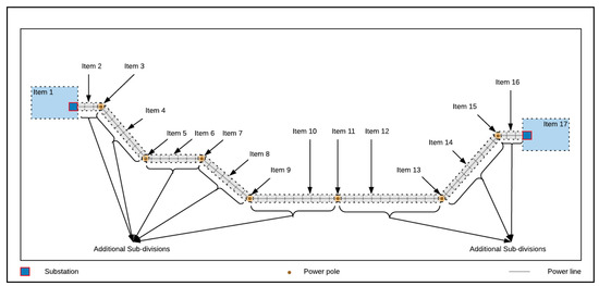
Figure 8.
Section subdivision of a schematic power grid. The items of interest consist here of the substations, the power poles, and the power line subsections (Aerial 2D view).
Figure 9 shows the item of interest chosen for the risk analysis. It furthermore illustrates the presence of trees along the power lines.
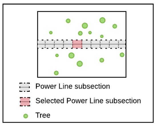
Figure 9.
Selection of a power-line subsection as an item of interest for a risk analysis. The existence of the vegetation hazard is indicated by the presence of trees in the surrounding of the power line (Aerial 2D view).
4.2. Reinforcement Action 2—Parameter Characterization and Data Source Identification
Three different dimensions can be reported when estimating the probability of outage due to a tree falling on a power line.:
- The physical configuration,
- The stability of the trees surrounding the power lines,
- External factors, such as strong winds.
The following parameters play a role in the definition of the physical configuration:
- Vegetation density/number of trees (*),
- Forest social configuration (i.e., distance characterization between trees),
- Height of tree (*),
- Structure of tree crown (depth),
- Structure of tree crown (width, diameter) (*),
- Terrain exposure to wind,
- X–Y direction from a tree to the power line,
- X–Y distance from a tree to the power line (*),
- Z-delta (intensity of altitude variation).
Table 18 reports the characterization we propose for the four parameters we selected in this case study designated by (*) in the preceding list.
Table 18.
Characterization of a subselection of parameters.
Identification of data sources able to provide information for the four retained parameters is then executed. LiDAR point clouds, orthophotos based on aerial images, and satellite-based orthophotos correspond to some of the relevant data sources. The complete list of preselected sources is reported in Appendix C. Appendix C also reports suggestions of preprocessing methods usable to link each data source to the selected parameters.
4.3. Three-Phases Method Application
The geolocation of the AoI integrating the item of interest is given in the ETRS89/UTM32N coordinate system as follows:
- Minimum easting (X): 610,205,
- Minimum northing (Y): 6,561,098,
- Maximum easting (X): 610,253,
- Maximum northing (Y): 6,561,122.
The risk analysis is assumed to be made on 1 December 2021.
We consider a selection of three datasets to evaluate the probability of outage due to tree falls on power lines: a LiDAR point cloud, an orthophoto based on aerial images, and a satellite-based orthophoto.
The chosen files correspond to simulated realistic datasets generated for the present study. We assume having used crosswalks where required, and we report, for each dataset, the equivalent of original DC terms necessary for the analysis in Table 19. Note that the nature of the considered files and the nature of the evaluated parameters lead the spatiotemporal characteristics (acquisition area, spatial resolution, etc.) considered in the present case study to similarly impact all addressed parameters. The outcome of each phase (i.e., the ranking of the datasets based on their estimated informative potential after the application of each phase) is summarized in a unique table (Table 25) at the end of Section 4.
Table 19.
DC-like terms for the three simulated datasets.
4.3.1. Default Maximum Potential of Knowledge (DMPK)
The knowledge acquired during learning phase 1 enabling one to report the DMPK is detailed per data source and per parameter in Table 20.
Table 20.
Meta-features phase 1—DMPK calculation per data source per parameter.
The scores obtained via the calculation of the DMPK for each data source and each parameter enable generating an initial ranking per parameter of the considered datasets, as described in Table 25.
4.3.2. First Degradation Factor (DF1)
Table 21 reports the results of calculations required for the quality assessment of (1) spatial inferred scene-related terms and (2) temporal inferred scene-related terms.
Table 21.
Inferred scene-related DC terms.
We characterize the contribution of the spatial information to the first degradation factor for each parameter informed by each of the retained dataset as reported in Table 22.
Table 22.
Meta-features phase 2—spatial contribution to DF1 per data source per parameter.
The spatial overlap’s nature justifies further proceeding with a temporal analysis of the degradation factor DF1.
We characterize the contribution of the temporal information to the first degradation factor for each parameter informed by each of the retained dataset as reported in Table 23. Note that the detailing of the temporal resolution TReds,pa, the temporal density TDeds,pa, the temporal distribution TDids,pa, and the temporal noise TNds,pa is not reported here because they were identified as not applicable on the basis of the calculation of temporal overlap utility TOUds,pa.
Table 23.
Meta-features phase 2—temporal contribution to DF1 per dataset per parameter.
We combine DF1a and DF1b to calculate the total degradation factor DF1. This enables calculating the updated potential of knowledge (PKDF1,ds,pa) per dataset and per parameter, as described in Table 25.
4.3.3. Second Degradation Factor (DF2)
Metadata relative to the objectives, the authors, and the circumstances of the data acquisition enable calculating the value of the second degradation factor for each of the datasets, as detailed in Table 24.
Table 24.
Meta-features phase 3—DF2 per dataset.
By applying the degradation factor DF2 and updating the calculation of the potential of knowledge (PKDF1,DF2,ds,pa) per dataset and per parameter, we obtain a final ranking of the best candidate dataset for each of the considered parameter, as described in Table 25.
Table 25.
Spatiotemporal- and trust-influenced informative potential assessment per datasets per parameter.
Table 25 details the evolution of the ranking of the best candidate for each parameter based on the application of the 3 phases mentioned in our method.
The coloring (green, yellow, orange) of the scores within each phase as detailed in Table 25 reports the first, second, and third best candidate datasets for the characterization of each parameter. Table 25 indicates that LiDAR-based point clouds initially constitute the most interesting type of dataset for the present case study. Therefore, they should be preferred by default, in the absence of any other type of information relative to file properties.
However, the application of the degradation factors DF1 and DF2 leads to a new ranking of the best candidate datasets for each considered parameter. In particular, the satellite-based orthophoto obtains the first position in the ranking for all parameters after the application of DF1 and keeps this position after application of DF2. The LiDAR point cloud obtains the second position for informing the parameter “height of tree” after the application of DF1 and keeps this position after application of DF2. The orthophoto based on aerial images obtains the third position for the characterization of the parameter “density/number of trees” after the application of DF1, but is reranked second after application of DF2.
5. Discussion
5.1. Method Benefits and Contribution for Risk Assessment
The accessibility to many data sources for risk assessment is a recent phenomenon for many application areas. While this consists of a great opportunity for data-driven assessments and DRA, the process for choosing one dataset to inform a parameter in detriment of another was not yet formalized. The method proposed in this paper formalizes this process. One of the main advantages of the method is the use of metadata; the method provides the ranking of the best datasets according to their informative potential without the need for the analyst to open the file and assess its content. In addition to identifying the best dataset for each parameter, the proposed approach also identifies the best parameters per source. Such information can be used as an additional indicator for strategical decision making when deciding about investments related to future data acquisitions.
The results of the method application are, to the best of our knowledge, representative of the reality that power-grid operators can face. The impact of the degradation factors highlights that a dataset originating from a less valued data source may be preferred to a dataset originating from an initially higher-ranked data source, the content of which is outdated or of too low quality. The results also show that, while getting degraded and losing its leading position to inform a specific parameter, a dataset may still remain the best choice for another parameter. This indicates the importance of assessing the informative potential of a dataset on a parameter level rather than as one block.
Moreover, the method provides flexibility for the analyst to achieve the following:
- Tune the meta-features used to calculate DMPK in phase 1, if expertise/follow-up gain of knowledge shows that the initial estimation was not adequate, the initial estimation needed to be updated, or if the evolution in technologies/competencies of stakeholders enables improving the initially obtainable quality of information;
- Adequately maintain elements required for the calculation of the trust-related meta-features by adding, confirming, or removing entities in the lists used for the calculation of the second degradation factor (e.g., new standard or withdraw of a previous standard);
- Have the process iterated over time (even without new datasets) and readapt the ranking of the considered sources if required;
- Modify the weights given to any of the meta-features proposed in phases 1, 2, and 3 on the basis of what one decides to be important or if new risk evidence implies that changes are required;
- Assess the potential of new types of data sources not yet known and integrate the related datasets into the risk analysis by running them through the three phases.
This approach, thus, supports the development and implementation of DRAs by ensuring proper and dynamic dataset selection in an environment with ever-increasing access to more information. It should be noted that the main benefits of the method are to be gained in a long-term application, i.e., when used after the first time, the analyst needs to update it only in case new data sources are considered.
5.2. Limitations and Further Requirements
5.2.1. Reliance on Metadata Format
The proposed method is particularly sensitive to metadata existence and quality. Yet, experience shows that metadata can be in the wrong format (i.e., not respecting existing standards), inexistent, or incomplete, as illustrated by the absence of some objective/author/circumstance-related terms in the case study. Metadata may also be corrupted and contain inaccurate information, due to human actions or inadequate automatic processing. Metadata in the wrong format may lead to more challenging and time-consuming conversions into DC terms, as one would have to work with/generate nonconventional crosswalks. As a partial solution, and assuming that the number of metadata terms is expected to remain limited, one may create lists of “standard-like” terms to convert non-standardized metadata into information usable for the method. In line with this concept, one could also generate further quality indicators of the observed datasets by implementing and counting alarms used to highlight missing metadata. Additionally, it might be strategic to enable one to assign some “privileges” to specific datasets to avoid naïvely degrading the value attributed to datasets due to absence of trust information in the metadata (for instance, for data originating from reference entities such as governmental-based institutions). Such approaches may also be considered when acknowledging that some datasets initially lack metadata but are known to have been generated internally and can, thus, be considered as more “trustable”.
Lastly, two additional approaches—optimistic or pessimistic—may be chosen to face incomplete metadata reporting, as applied in the presented case study. For the former, stakeholders can apply the minimum degradation and generate alerts for manual verification of the final ranking when missing information has been detected. Alternatively, stakeholders may be more conservative and apply the maximum degradation to minimize the possibilities of building on uncertainties. An optimistic approach was chosen for the calculation of the second degradation factor in our work. The pessimistic approach would have led to the same ranking in the present case study because of the metadata we decided to report for those simulated datasets. However, this may usually not be the case. The choice of the strategy to follow is a more subjective task that, thus, needs to be addressed on a case-by-case analysis and is hardly generalizable in the generic description of our approach.
5.2.2. Three-Phases Method Elements
The characterization of the properties in phases 1, 2, and 3 of the method mainly consists of the definition of classes and class boundaries relative to each property, according to the authors’ experience. Yet, the method provides sufficient flexibility for the boundaries to be adapted if needed, especially in a context other than power-grid management. The choices made in the definition of the three-phases method may, thus, be seen as an illustration of a general guideline that can be adapted to the context in which it is applied rather than as a rigid formulation.
The weights associated with the meta-features of each phase are likely to be different from application to application or from organization to organization. Although the approach is already implementable as is for any project where the requirements related to the learning phases are fulfilled, another implementation would require first defining the value of the reported weights. Different approaches may be considered for this purpose, and one may, for instance, tackle this problem as a meta-learning task. Alternatively, one could use more straightforward solutions such as the application of Zip’s law, as applied in other work [92].
We chose a normalized weighted sum to summarize the results of all the properties used for the definition of the DMPK and DFs. This choice is considered robust, well-known, and straightforward [93,94], and it was adopted for a first formulation of the proposed methodology. Multicriteria decision-making methods could also be considered, for instance, if further dependencies between properties were to be considered in future applications of the method. Furthermore, the approach considers, right now, all datasets to be independent and analyzed independently and not leveraging one another. Future extensions should address the existence of links between datasets.
The implementation of the method is more labor-intensive in the first iterations of the process, especially when the knowledge of the involved stakeholders needs to be converted into information exploitable for the use of the presented method. Verifications required after detecting new terms in the lists used to calculate the second degradation factor may be particularly time-consuming. However, this workload and the general need for manual verifications are expected to diminish over time as the number of processed datasets increases, facilitating future automatic processing.
6. Conclusions
Despite being synonymous with considerable advantages, increasing data availability related to energy systems also implies numerous challenges from a data management perspective. In the present work, we suggest an approach enabling to tackle such challenges in the risk analysis field by analyzing features that may degrade the information potential of a dataset compared to a baseline (default maximum potential of knowledge (DMPK)). The key contributions of this research are twofold. First, it proposes a method for reinforcing data-related risk analysis steps. The use of this method ensures that risk analysts can methodically identify and assess the available data for informing the risk analysis key parameters. Second, it develops a method for selecting the best datasets according to their informative potential. The method, thus, formalizes, in a traceable and reproducible manner, the process for choosing one dataset to inform a parameter in detriment of another, which can lead to more accurate risk analyses.
The application of the method to vegetation-related risk assessment in power grids shows that the approach enables dynamically selecting the best information possible. It also demonstrates that a dataset originating from an initially less valued data source (the satellite-based orthophoto) may be preferred to a dataset originating from a higher-ranked data source, the content of which is outdated or of too low quality (LiDAR-based point clouds).
The proposed method reduces approximations and uncertainties in risk analysis by improving tracing of information and measurement characterization, thereby supporting the optimization of dataset preparation and integration for more efficient risk assessments. The generic aspect of the approach opens up further applications, such as management of safety barriers or risk management applied in other areas such as finance or insurance, which can also access large data lakes. The method is particularly valuable for the risk assessment of large-scale “open” systems, subject to environmental changes and presenting increasing opportunities for data capture. Such systems include not only power grids, but also transportation systems and gas pipelines. In addition to pressure, temperature, and flow sensors that might identify a failure after a leak is already established, external pipelines can benefit from data captured by autonomous systems (drones) or satellites for identifying a growing crack that can potentially result in a leak.
Lastly, although the exploitation of natural language processing techniques may in the future further support the application of the method (i.e., via advanced text-based quality assessment of metadata), there is an undiscussable need for proper and better metadata registration and maintenance. The community should encourage good practices in this direction, and our work can be used to illustrate the potential benefits of doing so.
Author Contributions
Conceptualization, M.F.P., M.R., D.R. and N.P.; methodology, M.F.P., M.R. and N.P.; validation, M.F.P., M.R., D.R., C.T.E. and N.P.; formal analysis, M.F.P.; investigation, M.F.P.; data curation, M.F.P.; writing—original draft preparation, M.F.P.; writing—review and editing, M.R., D.R., C.T.E. and N.P.; supervision, D.R. and N.P.; project administration, N.P.; funding acquisition, D.R. and N.P. All authors have read and agreed to the published version of the manuscript.
Funding
This work is part of the project “Dynamic risk management for smart grids in large-scale interconnected power systems”, funded by eSmart Systems and the Norwegian Research Council (Nærings PhD program, Project No.: 276404), which the authors would like to thank for their support.
Data Availability Statement
Not applicable.
Conflicts of Interest
The authors declare no conflict of interest. The funders had no role in the design of the study; in the collection, analyses, or interpretation of data; in the writing of the manuscript, or in the decision to publish the results.
Appendix A
Table A1 reports an extract of the “open directory of metadata standards applicable to scientific data” [35], provided by the Metadata Standards Directory Working Group [33], a working group from the Research Data Alliance [34]. The directory is community-maintained.
Table A1.
Extract of commonly used metadata standards [35].
Table A1.
Extract of commonly used metadata standards [35].
| Name | Original Field of Application | Description | Link to Resource |
|---|---|---|---|
| MARC | Arts and humanities | MARC (machine-readable cataloging) is a standard mostly originally used for reporting and exchanging bibliographic records. | http://www.loc.gov/marc/ (accessed on 15 February 2022) |
| Darwin Core | Life sciences | A body of standards used for reporting and exchanging biology-related information. | http://rs.tdwg.org/dwc/index.htm (accessed on 15 February 2022) |
| EML | Life sciences | EML (ecological metadata language) is a metadata specification used for reporting and exchanging ecology-related information | https://nceas.github.io/eml/ (accessed on 15 February 2022) |
| ISO 19115 | Physical sciences and mathematics | ISO 19115 (geographic information—metadata) is schema used for the description of geographic information and services. | https://www.iso.org/standard/26020.html (accessed on 15 February 2022) https://www.iso.org/standard/53798.html (accessed on 15 February 2022) |
| Dublin Core | General research data | Authoritative specification of all metadata terms maintained by the Dublin Core™ Metadata Initiative (DCMI). These terms are intended to be used in combination with metadata terms from other, compatible vocabularies. | http://dublincore.org (accessed on 15 February 2022) |
Appendix B
Table A2, Table A3 and Table A4 detail the recategorization of the DC terms relevant for a risk analysis into three classes: (1) file (nature of the dataset), (2) scene (site-/time-specifications of the dataset), and (3) objectives/author/circumstances (agents and factors influencing data management). The tables also report the respective definition of each of the selected terms [83] (The reader is directed to the home page of the Dublin Core™ Metadata Initiative for a complete description of the terms not used in the present paper.).
Table A2.
File-related DC terms.
Table A2.
File-related DC terms.
| N° | Term | Definition |
|---|---|---|
| 1-1 | Format | The file format, physical medium, or dimensions of the resource. |
| 1-2 | Type | The nature or genre of the resource. |
Table A3.
Scene-related DC terms.
Table A3.
Scene-related DC terms.
| N° | Term | Definition |
|---|---|---|
| 2.1 | Coverage | The spatial or temporal topic of the resource, spatial applicability of the resource, or jurisdiction under which the resource is relevant. |
| 2.2-a | Spatial | Spatial characteristics of the resource (sub-property of coverage). |
| 2.3-b | Temporal | Temporal characteristics of the resource (sub-property of coverage). |
| 2.4-b | Date | A point or period of time associated with an event in the lifecycle of the resource. |
| 2.5-b | Created | Date of creation of the resource (sub-property of date). |
| 2.6-b | Issued | Date of formal issuance of the resource (sub-property of date). |
| 2.7-b | AccrualPeriodicity | The frequency with which items are added to a collection. |
| 2.8-b | Available | Date that the resource became or will become available (sub-property of date). |
| 2.9-b | Modified | Date on which the resource was changed (sub-property of date). |
| 2.10-b | Valid | Date (often a range) of validity of a resource (sub-property of date). |
| 2.11-b | DateCopyrighted | Date of copyright of the resource (sub-property of date). |
| 2.12-b | DateSubmitted | Date of submission of the resource (sub-property of date). |
| 2.13-b | DateAccepted | Date of acceptance of the resource (sub-property of date). |
Table A4.
Objective/author/circumstance-related DC-terms.
Table A4.
Objective/author/circumstance-related DC-terms.
| N° | Term | Definition |
|---|---|---|
| 3.1 | Audience | A class of agents for whom the resource is intended or useful. |
| 3.2 | Abstract | A summary of the resource. |
| 3.3 | AccrualMethod | The method by which items are added to a collection. |
| 3.4 | BibliographicCitation | A bibliographic reference for the resource. |
| 3.5 | ConformsTo | An established standard to which the described resource conforms. |
| 3.6 | Contributor | An entity responsible for making contributions to the resource. |
| 3.7 | Creator | An entity responsible for making the resource. |
| 3.8 | Description | An account of the resource. |
| 3.9 | EducationLevel | A class of agents, defined in terms of progression through an educational or training context, for which the described resource is intended. |
| 3.10 | Extent | The size or duration of the resource. |
| 3.11 | HasVersion | A related resource that is a version, edition, or adaptation of the described resource. |
| 3.12 | IsReferencedBy | A related resource that references, cites, or otherwise points to the described resource. |
| 3.13 | IsReplacedBy | A related resource that supplants, displaces, or supersedes the described resource. |
| 3.14 | IsVersionOf | A related resource of which the described resource is a version, edition, or adaptation. |
| 3.15 | Provenance | A statement of any changes in ownership and custody of the resource since its creation that are significant for its authenticity, integrity, and interpretation. |
| 3.16 | Publisher | An entity responsible for making the resource available. |
| 3.17 | References | A related resource that is referenced, cited, or otherwise pointed to by the described resource. |
| 3.18 | Replaces | A related resource that is supplanted, displaced, or superseded by the described resource. |
| 3.19 | Source | A related resource from which the described resource is derived. |
| 3.20 | Subject | A topic of the resource. |
| 3.21 | Title | A name given to the resource. |
Appendix C
Table A5 lists all data sources identified as able to provide information for the four parameters retained in the case study. The table also reports suggestions of preprocessing methods usable to link each data source to the selected parameters.
Identical cells in the table are merged where possible for consistency purposes. The value of the information that can be provided by each of the retained sources is detailed in the application of the method presented in Section 4.
Table A5.
Suggestions of preprocessing methods usable to link the data sources to the selected parameters.
Table A5.
Suggestions of preprocessing methods usable to link the data sources to the selected parameters.
| Data Source | Density/Number of Trees | Height of Tree | Structure of Tree Crown (Width, Diameter) | X–Y Distance from a Tree to the Power Line |
|---|---|---|---|---|
| Aerial optical inspection images | Visual estimation, counting | Visual estimation, classification | ||
| Forest survey (map) | Average value reported over a pixel | - | ||
| LiDAR point clouds | Cloud segmentation and counting or point cloud density calculation | Cloud segmentation and measurement | ||
| Meshed photogrammetry-based point clouds | Evaluation of number, depth, and relative proportion of valleys | Mesh segmentation and measurement | ||
| Orthophotos (aerial images) | Counting, counting per area | Visual estimation, extrapolated from crown width | Crown size measurement | Distance measurement tree-power line |
| Orthophotos (satellite images) | Counting, counting per area | Visual estimation, extrapolated from crown width | Crown size estimation | Distance estimation tree, power line |
| Pests/fungi survey (map) | Probabilistic estimation based on pests/fungi-related damages over time | - | ||
| Photogrammetry point clouds | Cloud segmentation and counting or point cloud density calculation | Cloud segmentation and measurement | ||
| Soil survey (map) | Probabilistic estimation of having a tree based on soil type | Probabilistic estimation of having a tree and estimation of growth potential for trees depending on soil type | - | |
| TOPEX (topographical wind exposure) (map) | Probabilistic estimation of having a tree and estimation of growth potential for trees depending on altitude + probable wind impact over time | Probabilistic estimation of having a tree and estimation of growth potential for trees depending on altitude + probable wind impact over time + Z-delta measurement for difference due to terrain variations | ||
| Topography (map) | Probabilistic estimation of having a tree and estimation of growth potential for trees depending on altitude | Probabilistic estimation of having a tree and estimation of growth potential for trees depending on altitude + Z-delta measurement for difference due to terrain variations | ||
| Weather historical data | Probabilistic estimation of having a tree and estimation of growth potential for trees depending on weather conditions | - | ||
References
- Zúñiga, A.A.; Baleia, A.; Fernandes, J.; Branco, P.J.D.C. Classical Failure Modes and Effects Analysis in the Context of Smart Grid Cyber-Physical Systems. Energies 2020, 13, 1215. [Google Scholar] [CrossRef]
- Zhang, Z.; Yang, H.; Yin, X.; Han, J.; Wang, Y.; Chen, G. A Load-Shedding Model Based on Sensitivity Analysis in on-Line Power System Operation Risk Assessment. Energies 2018, 11, 727. [Google Scholar] [CrossRef]
- Kumar, G.V.B.; Sarojini, R.K.; Palanisamy, K.; Padmanaban, S.; Holm-Nielsen, J.B. Large Scale Renewable Energy Integration: Issues and Solutions. Energies 2019, 12, 1996. [Google Scholar] [CrossRef]
- Pacevicius, M.; Roverso, D.; Rossi, P.S.; Paltrinieri, N. Smart grids: Challenges of processing heterogeneous data for risk assessment. In Proceedings of the 14th International Conference on Probabilistic Safety Assessment and Management, Los Angeles, CA, USA, 16–21 September 2018. [Google Scholar]
- Pacevicius, M.; Ramos, M.A.; Paltrinieri, N. Optimizing Technology-based Decision-support for management of Infrastructures under risk: The Case of Power Grids. In Proceedings of the 30th ESREL-15th PSAM, Venice, Italy, 1–5 November 2020; Research Publishing: Singapore, 2020; p. 8. [Google Scholar] [CrossRef]
- Ciapessoni, E.; Cirio, D.; Pitto, A.; Marcacci, P.; Lacavalla, M.; Massucco, S.; Silvestro, F.; Sforna, M. A Risk-Based Methodology and Tool Combining Threat Analysis and Power System Security Assessment. Energies 2018, 11, 83. [Google Scholar] [CrossRef]
- Sayed, A.; El-Shimy, M.; El-Metwally, M.; Elshahed, M. Reliability, Availability and Maintainability Analysis for Grid-Connected Solar Photovoltaic Systems. Energies 2019, 12, 1213. [Google Scholar] [CrossRef]
- Elsisi, M.; Tran, M.-Q.; Mahmoud, K.; Lehtonen, M.; Darwish, M.M.F. Deep Learning-Based Industry 4.0 and Internet of Things towards Effective Energy Management for Smart Buildings. Sensors 2021, 21, 1038. [Google Scholar] [CrossRef] [PubMed]
- Tran, M.-Q.; Elsisi, M.; Mahmoud, K.; Liu, M.-K.; Lehtonen, M.; Darwish, M.M.F. Experimental Setup for Online Fault Diagnosis of Induction Machines via Promising IoT and Machine Learning: Towards Industry 4.0 Empowerment. IEEE Access 2021, 9, 115429–115441. [Google Scholar] [CrossRef]
- Elsisi, M.; Tran, M.; Mahmoud, K.; Mansour, D.A.; Lehtonen, M.; Darwish, M.M. Towards Secured Online Monitoring for Digitalized GIS Against Cyber-Attacks Based on IoT and Machine Learning. IEEE Access 2021, 9, 78415–78427. [Google Scholar] [CrossRef]
- Zhang, D.; Qian, L.; Mao, B.; Huang, C.; Huang, B.; Si, Y. A Data-Driven Design for Fault Detection of Wind Turbines Using Random Forests and Xgboost. IEEE Access 2018, 6, 21020–21031. [Google Scholar] [CrossRef]
- Beerens, H.; Post, J.; Uijtdehaag, P. The use of generic failure frequencies in QRA: The quality and use of failure frequencies and how to bring them up-to-date. J. Hazard. Mater. 2006, 130, 265–270. [Google Scholar] [CrossRef][Green Version]
- Villa, V.; Paltrinieri, N.; Khan, F.; Cozzani, V. Towards dynamic risk analysis: A review of the risk assessment approach and its limitations in the chemical process industry. Saf. Sci. 2016, 89, 77–93. [Google Scholar] [CrossRef]
- Paltrinieri, N.; Khan, F.; Cozzani, V. Coupling of advanced techniques for dynamic risk management. J. Risk Res. 2015, 18, 910–930. [Google Scholar] [CrossRef]
- Paltrinieri, N.; Khan, F.I. Dynamic risk analysis—Fundamentals. In Advanced Methods of Risk Assessment and Management; Khan, F.I., Amyotte, P.R., Eds.; Elsevier: Amsterdam, The Netherlands, 2020; Volume 4, pp. 35–60. [Google Scholar]
- Pacevicius, M.; Paltrinieri, N.; Thieme, C.A.; Rossi, P.S. Addressing the Importance of Data Veracity during Data Acquisition for Risk Assessment Processes. In Proceedings of the 67th Annual Reliability and Maintainability Symposium, Orlando, FL, USA, 24–27 May 2021; p. 7. [Google Scholar] [CrossRef]
- Xing, J.; Zeng, Z.; Zio, E. A framework for dynamic risk assessment with condition monitoring data and inspection data. Reliab. Eng. Syst. Saf. 2019, 191, 106552. [Google Scholar] [CrossRef]
- Chen, N.; Liu, W.; Bai, R.; Chen, A. Application of computational intelligence technologies in emergency management: A literature review. Artif. Intell. Rev. 2019, 52, 2131–2168. [Google Scholar] [CrossRef]
- ISO 31000:2018; Risk Management—Guidelines. International Standardization Organization (ISO): Geneva, Switzerland, 2018; p. 34.
- Gazzea, M.; Pacevicius, M.; Dammann, D.O.; Sapronova, A.; Lunde, T.M.; Arghandeh, R. Automated Power Lines Vegetation Monitoring using High-Resolution Satellite Imagery. Trans. Power Deliv. 2021, 37, 308–316. [Google Scholar] [CrossRef]
- Pacevicius, M.; Gazzea, M.; Dammann, D.O.; Sapronova, A.; Lunde, T.M.; Arghandeh, R. GridEyeS Deliverable D3: Technical Feasibility Assessment; StormGeo: Bergen, Norway, 2020. [Google Scholar]
- Pacevicius, M.; Haskins, C.; Paltrinieri, N. Supporting the Application of Dynamic Risk Analysis to Real-World Situations using Systems Engineering: A focus on the Norwegian Power Grid Management. In Recent Trends and Advances in Model Based Systems Engineering; Springer: Cham, Switerland, 2022. [Google Scholar] [CrossRef]
- Merriam-Webster Metadata. Merriam-Webster.com Dictionary. 2022. Available online: https://www.merriam-webster.com/dictionary/metadata (accessed on 15 February 2022).
- Wierling, A.; Schwanitz, V.J.; Altinci, S.; Bałazińska, M.; Barber, M.J.; Biresselioglu, M.E.; Burger-Scheidlin, C.; Celino, M.; Demir, M.H.; Dennis, R.; et al. FAIR Metadata Standards for Low Carbon Energy Research—A Review of Practices and How to Advance. Energies 2021, 14, 6692. [Google Scholar] [CrossRef]
- Song, G.; Nie, Y.; Chen, G.; Liu, X. Applied research of data-driven multi-level reliability model in transportation safety risk evaluation. In Proceedings of the 2020 International Conference on Big Data, Artificial Intelligence and Internet of Things Engineering (ICBAIE), Fuzhou, China, 12–14 June 2020; pp. 116–121. [Google Scholar]
- ISO/IEC 11179-3:2013; Information Technology—Metadata Registries (MDR)—Part 3: Registry Metamodel and Basic Attributes. International Standardization Organization (ISO): Geneva, Switzerland, 2013; p. 227.
- Wang, H.; Ye, Z. An ETL services framework based on metadata. In Proceedings of the 2010 2nd International Workshop on Intelligent Systems and Applications, Wuhan, China, 22–23 May 2010. [Google Scholar] [CrossRef]
- Bordogna, G.; Carrara, P.; Pagani, M.; Pepe, M.; Rampini, A. Managing imperfect temporal metadata in the catalog services of Spatial Data Infrastructures compliant with INSPIRE. In Proceedings of the 2009 International Fuzzy Systems Association World Congress and 2009 European Society for Fuzzy Logic and Technology Conference, Lisbon, Portugal, 20–24 July 2009; pp. 915–920. [Google Scholar]
- Lambe, P. Organising Knowledge: Taxonomies, Knowledge and Organisational Effectiveness; Chandos Publishing: Oxford, UK, 2007; ISBN 9781843342274. [Google Scholar]
- Burnett, K.; Ng, K.B.; Park, S. A comparison of the two traditions of metadata development. J. Am. Soc. Inf. Sci. 1999, 50, 1209–1217. [Google Scholar] [CrossRef]
- Working Group on Research Data—Science Europe (SE) Metadata. Available online: http://sedataglossary.shoutwiki.com/wiki/Metadata (accessed on 15 February 2022).
- Data on the Web Best Practices Working Group—World Wide Web Consortium (W3C) Guidance on the Provision of Metadata. Available online: https://www.w3.org/2013/dwbp/wiki/Guidance_on_the_Provision_of_Metadata (accessed on 15 February 2022).
- Harrison, M.; Farias Lóscio, B. Re: Intrinsic vs. Extrinsic Metadata (My Action #54). Available online: https://lists.w3.org/Archives/Public/public-dwbp-wg/2014Jul/0004.html (accessed on 15 February 2022).
- Wang, R.Y.; Strong, D.M. Beyond accuracy: What data quality means to data consumers. J. Manag. Inf. Syst. 1996, 12, 5–33. [Google Scholar] [CrossRef]
- Research Data Alliance Metadata Standards Directory WG. Available online: https://www.rd-alliance.org/groups/metadata-standards-directory-working-group.html (accessed on 15 February 2022).
- Research Data Alliance. Available online: https://www.rd-alliance.org (accessed on 15 February 2022).
- Chen, S.; Alderete, K.A.; Ball, A. RDA Metadata Standards Directory. Available online: https://rd-alliance.github.io/metadata-directory/ (accessed on 15 February 2022).
- World Wide Web Consortium (W3C) Semantic Web. Available online: https://www.w3.org/standards/semanticweb/ (accessed on 15 February 2022).
- Zaveri, A.; Rula, A.; Maurino, A.; Pietrobon, R.; Lehmann, J.; Auer, S. Quality assessment for Linked Data: A Survey A systematic literature review and conceptual framework. Semant. Web 2016, 7, 63–93. [Google Scholar] [CrossRef]
- American Society for Information Science and Technology Dublin Core™ Metadata Initiative. Available online: https://www.dublincore.org/collaborations/asist/ (accessed on 15 February 2022).
- Weibel, S. The Dublin core: A simple content description model for electronic resources. Bull. Am. Soc. Inf. Sci. 1997, 24, 9–11. [Google Scholar] [CrossRef]
- ISO 15836-1:2017; Information and Documentation—The Dublin Core Metadata Element Set—Part 1: Core Elements. International Standardization Organization (ISO): Geneva, Switzerland, 2017; p. 7.
- ANSI/NISO Z39.85; The Dublin Core Metadata Element Set. National Information Standards Organization: Baltimore, MD, USA, 2012; p. 7.
- ISO 15836-2:2019; Information and Documentation—The Dublin Core Metadata Element Set—Part 2: DCMI Properties and Classes. International standardization Organization (ISO): Geneva, Switzerland, 2019; p. 26.
- Dublin Core™ Metadata Initiative DCMI Metadata Terms. Available online: https://www.dublincore.org/ (accessed on 15 February 2022).
- Woodley, M.S. Crosswalks, Metadata Harvesting, Federated Searching, Metasearching: Using Metadata to Connect Users and Information; Getty Research Institute: Los Angeles, CA, USA, 2008; pp. 1–25. [Google Scholar]
- Harpring, P. Metadata Standards Crosswalks; Getty Research Institute: Los Angeles, CA, USA, 2022. [Google Scholar]
- Metadata Working Group of the Emory University Crosswalk of Core Metadata. Available online: https://metadata.emory.edu/guidelines/descriptive/crosswalk.html (accessed on 15 February 2022).
- Leahey, A.; Barsky, E.; Brosz, J.; Garnett, A.; Gray, V.; Hafner, J.; Handren, K.; Harrigan, A.; Lacroix, C.; Pascoe, J.; et al. Metadata for Discovery: Disciplinary Standards and Crosswalk Progress Report; University of British Columbia Library: Vancouver, BC, USA, 2017. [Google Scholar]
- Kaplan, S.; Garrick, B.J. On The Quantitative Definition of Risk. Risk Anal. 1981, 1, 11–27. [Google Scholar] [CrossRef]
- NORSOK Standard Z-013; Risk and Emergency Preparedness Assessment. NORSOK: Lysaker, Norway, 2010.
- CAN/CSA-Q850-97 (R2009); Risk Management: Guideline for Decision Makers. Canadian Standards Association (CSA): Ottawa, ON, Canada, 1997.
- De Marchi, B.; Ravetz, J.R. Risk management and governance: A post-normal science approach. Futures 1999, 31, 743–757. [Google Scholar] [CrossRef]
- Aven, T.; Krohn, B.S. A new perspective on how to understand, assess and manage risk and the unforeseen. Reliab. Eng. Syst. Saf. 2014, 121, 1–10. [Google Scholar] [CrossRef]
- Paltrinieri, N.; Dechy, N.; Salzano, E.; Wardman, M.; Cozzani, V. Towards a new approach for the identification of atypical accident scenarios. J. Risk Res. 2013, 16, 337–354. [Google Scholar] [CrossRef]
- Paltrinieri, N.; Khan, F.; Amyotte, P.; Cozzani, V. Dynamic approach to risk management: Application to the Hoeganaes metal dust accidents. Process Saf. Environ. Prot. 2013, 92, 669–679. [Google Scholar] [CrossRef]
- Kalantarnia, M.; Khan, F.; Hawboldt, K. Dynamic risk assessment using failure assessment and Bayesian theory. J. Loss Prev. Process Ind. 2009, 22, 600–606. [Google Scholar] [CrossRef]
- Khakzad, N.; Khan, F.; Amyotte, P. Dynamic risk analysis using bow-tie approach. Reliab. Eng. Syst. Saf. 2012, 104, 36–44. [Google Scholar] [CrossRef]
- Bucelli, M.; Paltrinieri, N.; Landucci, G. Integrated risk assessment for oil and gas installations in sensitive areas. Ocean Eng. 2018, 150, 377–390. [Google Scholar] [CrossRef]
- Lee, S.; Landucci, G.; Reniers, G.; Paltrinieri, N. Validation of dynamic risk analysis supporting integrated operations across systems. Sustainability 2019, 11, 6745. [Google Scholar] [CrossRef]
- Yang, X.; Haugen, S.; Paltrinieri, N. Clarifying the concept of operational risk assessment in the oil and gas industry. Saf. Sci. 2018, 108, 259–268. [Google Scholar] [CrossRef]
- JCGM 200:2012; International Vocabulary of Metrology—Basic and General Concepts and Associated Terms (VIM). Joint Committee for Guides in Metrology (JCGM): Sèvres, France, 2012.
- ISO 10012:2003; Measurement Management Systems—Requirements for Measurement Processes and Measuring Equipment. International Standardization Organization (ISO): Geneva, Switzerland, 2003; p. 26.
- Dillon, R.L.; Paté-Cornell, M.E.; Guikema, S.D. Programmatic risk analysis for critical engineering systems under tight resource constraints. Oper. Res. 2003, 51, 354–370. [Google Scholar] [CrossRef]
- Borgonovo, E.; Cillo, A. Deciding with Thresholds: Importance Measures and Value of Information. Risk Anal. 2017, 37, 1828–1848. [Google Scholar] [CrossRef] [PubMed]
- Iwanaga, T.; Wang, H.H.; Hamilton, S.H.; Grimm, V.; Koralewski, T.E.; Salado, A.; Elsawah, S.; Razavi, S.; Yang, J.; Glynn, P.; et al. Socio-technical scales in socio-environmental modeling: Managing a system-of-systems modeling approach. Environ. Model. Softw. 2021, 135, 104885. [Google Scholar] [CrossRef] [PubMed]
- Stefana, E.; Cocca, P.; Marciano, F.; Rossi, D.; Tomasoni, G. A review of energy and environmental management practices in cast iron foundries to increase sustainability. Sustainability 2019, 11, 7245. [Google Scholar] [CrossRef]
- Paté-Cornell, M.E. Uncertainties in risk analysis: Six levels of treatment. Reliab. Eng. Syst. Saf. 1996, 54, 95–111. [Google Scholar] [CrossRef]
- Raussand, M. Risk Assessment—Theory, Methods, and Applications; Wiley: Hoboken, NJ, USA, 2011; Volume 1, ISBN 978-0-470-63764-7. [Google Scholar]
- Creedy, G.D. Quantitative risk assessment: How realistic are those frequency assumptions? J. Loss Prev. Process Ind. 2011, 24, 203–207. [Google Scholar] [CrossRef]
- Batini, C.; Cappiello, C.; Francalanci, C.; Maurino, A. Methodologies for Data Quality Assessment and Improvement. ACM Comput. Surv. 2009, 41, 52. [Google Scholar] [CrossRef]
- Wang, R.Y. A Product Perspective on Total Data Quality Management. Commun. ACM 1998, 41, 58–65. [Google Scholar] [CrossRef]
- English, L.P. Improving Data Warehouse and Business Information Quality: Methods for Reducing Costs and Increasing Profits; Wiley: Hoboken, NJ, USA, 1999; ISBN 978-0-471-25383-9. [Google Scholar]
- Eppler, M.J.; Helfert, M. A classification and analysis of data quality costs. In Proceedings of the International Conference on Information Quality, Cambridge, MA, USA, 5–7 November 2004; pp. 311–325. [Google Scholar]
- Loshin, D. (Ed.) 4-Economic framework of data quality and the value proposition. In Enterprise Knowledge Management; Academic Press: Cambridge, MA, USA, 2001; pp. 73–99. ISBN 9780124558403. [Google Scholar]
- Scannapieco, M.; Virgillito, A.; Marchetti, C.; Mecella, M.; Baldoni, R. The DaQuinCIS architecture: A platform for exchanging and improving data quality in cooperative information systems. Inf. Syst. 2004, 29, 551–582. [Google Scholar] [CrossRef]
- Long, J.A.; Seko, C.E. A Cyclic-Hierarchical Method for Database Data-Quality Evaluation and Improvement. In Information Quality; Wang, R.Y., Pierce, E.M., Madnick, S., Fisher, C., Eds.; Taylor & Francis Group: New York, NY, USA, 2005; p. 15. ISBN 9781315703480. [Google Scholar]
- Jeusfeld, M.A.; Quix, C.; Jarke, M. Design and Analysis of Quality Information for Data Warehouses. In Proceedings of the 17th International Conference on Conceptual Modeling, Singapore, 16–19 November 1998; pp. 349–362. [Google Scholar]
- Aljumaili, M.; Karim, R.; Tretten, P. Metadata-based data quality assessment. VINE J. Inf. Knowl. Manag. Syst. 2016, 46, 232–250. [Google Scholar] [CrossRef]
- European Space Imaging Our Satellites. Available online: https://www.euspaceimaging.com/ (accessed on 15 February 2022).
- Van Etten, A. You Only Look Twice: Rapid Multi-Scale Object Detection In Satellite Imagery. arXiv 2018, arXiv:1805.09512. [Google Scholar]
- Kuželka, K.; Slavík, M.; Surový, P. Very High Density Point Clouds from UAV Laser Scanning for Automatic Tree Stem Detection and Direct Diameter Measurement. Remote Sens. 2020, 12, 1236. [Google Scholar] [CrossRef]
- Dokic, T.; Kezunovic, M. Predictive Risk Management for Dynamic Tree Trimming Scheduling for Distribution Networks. IEEE Trans. Smart Grid 2018, 10, 4776–4785. [Google Scholar] [CrossRef]
- Alabri, A.; Hunter, J. Enhancing the quality and trust of citizen science data. In Proceedings of the 6th IEEE International Conference on E-Science (E-Science 2010), Brisbane, QLD, Australia, 7–10 December 2010; pp. 81–88. [Google Scholar] [CrossRef]
- Byabazaire, J.; O’Hare, G.; Delaney, D. Data quality and trust: A perception from shared data in IoT. In Proceedings of the IEEE International Conference on Communications, Dublin, Ireland, 7–11 June 2020. [Google Scholar] [CrossRef]
- Khakzad, N.; Khakzad, S.; Khan, F. Probabilistic risk assessment of major accidents: Application to offshore blowouts in the Gulf of Mexico. Nat. Hazards 2014, 74, 1759–1771. [Google Scholar] [CrossRef]
- Keßler, C.; de Groot, R.T.A. Trust as a Proxy Measure for the Quality of Volunteered Geographic Information in the Case of OpenStreetMap; Lecture Notes in Geoinformation and Cartography; Elsevier: Amsterdam, The Netherlands, 2013; Volume 2013, pp. 21–37. ISBN 9783319006147. [Google Scholar]
- Bovee, M.; Srivastava, R.P.; Mak, B. A conceptual framework and belief-function approach to assessing overall information quality. Int. J. Intell. Syst. 2003, 18, 51–74. [Google Scholar] [CrossRef]
- Pacevicius, M.; Roverso, D.; Rossi, P.S.; Paltrinieri, N. Risk of crack formation in power grid wooden poles and relationship with meteorological conditions: A Norwegian case study. In Proceedings of the Safety and Reliability—Safe Societies in a Changing World, Trondheim, Norway, 17–21 June 2018; pp. 1527–1533, ISBN 978-0-8153-8682-7. [Google Scholar]
- Alhelou, H.H.; Hamedani-Golshan, M.E.; Njenda, T.C.; Siano, P. A survey on power system blackout and cascading events: Research motivations and challenges. Energies 2019, 12, 682. [Google Scholar] [CrossRef]
- Pacevicius, M.; Dammann, D.O.; Gazzea, M.; Sapronova, A. Heterogeneous Data-merging Platform for Improved Risk Management in Power Grids. In Proceedings of the 67th Annual Reliability and Maintainability Symposium, Orlando, FL, USA, 24–27 May 2021; p. 7. [Google Scholar] [CrossRef]
- Bucelli, M.; Landucci, G.; Haugen, S.; Paltrinieri, N.; Cozzani, V. Assessment of safety barriers for the prevention of cascading events in oil and gas offshore installations operating in harsh environment. Ocean Eng. 2018, 158, 171–185. [Google Scholar] [CrossRef]
- Marler, R.T.; Arora, J.S. The weighted sum method for multi-objective optimization: New insights. Struct. Multidiscip. Optim. 2010, 41, 853–862. [Google Scholar] [CrossRef]
- Triantaphyllou, E. Multi-Criteria Decision Making Methods. In Multi-Criteria Decision Making Methods: A Comparative Study; Applied Optimization; Springer: Boston, MA, USA, 2000; Volume 44, p. 16. [Google Scholar] [CrossRef]


Publisher’s Note: MDPI stays neutral with regard to jurisdictional claims in published maps and institutional affiliations. |
© 2022 by the authors. Licensee MDPI, Basel, Switzerland. This article is an open access article distributed under the terms and conditions of the Creative Commons Attribution (CC BY) license (https://creativecommons.org/licenses/by/4.0/).