Self-Sensing Control of Open-End Winding PMSMs Fed by an Asymmetrical Hybrid Multilevel Inverter

Abstract

The paper presents a self-sensing control technique for a special type of multilevel motor drive featuring an Open-end Winding Permanent-Magnet Synchronous Motor fed on one side by a main multilevel inverter (MLI) and on the other side by an auxiliary two-level inverter (TLI). In order to minimize the power losses, the MLI manages the machine active power operating at a low-switching frequency. The TLI instead acts as an active power filter and operates at a higher switching frequency and a lower DC-Bus voltage than the MLI. The current control task is shared between the two inverters, as a predictive action is exerted by the MLI, while a feedback action is accomplished by the TLI. Common sensorless rotor position estimation techniques cannot be straightforwardly applied on such a system, due to the particular drive structure. Therefore, a specific technique has been carried out, able to ensure satisfactory efficiency and control performance in all the operating speed ranges by optimally exploiting the different features of the two inverters. Simulation and experimental results confirm the effectiveness of the proposed approach.

1. Introduction

Multilevel converters, exploiting mature medium-power semiconductor technologies, represent a viable solution for high power applications such as motor drives, wind and photovoltaic generators, electric propulsion systems and static VAR compensators [1,2,3,4,5]. They overcome some limitations of conventional three-phase two-level inverters in handling high voltages, high dv⁄dt levels and high switching frequencies fs > 1 kHz [6,7,8,9]. Among conventional multilevel inverter topologies, the Open-end Winding (OW) configuration has gained an increasing interest in recent years [10,11,12,13,14]. This configuration features a redundancy of the space-vector combinations, the absence of neutral point fluctuations, a reduction of the phase current ripple and an increased maximum stator voltage amplitude [15].

Sensorless operation of MLI motor drives are highly required in low and medium voltage applications in hostile environment, or where a wide speed range is required with rated load torque and soft-starting [16,17]. Self-sensing, or sensorless, control of AC machines has been extensively addressed in the last decades [18,19,20,21,22,23,24,25,26,27,28,29,30,31], due to cost and reliability advantages resulting from the elimination of cabling and mechanical sensors. Sensorless techniques able to estimate the rotor position, and speed in AC machines can be divided into two main groups: those dealing with the back-EMF/linkage flux estimation [24,25,26,27,28,29,30] and those dealing with spatial saliencies [18,26].

Sensorless techniques which rely upon back-EMF estimation can be exploited on multilevel motor drives even if they are operated at a low switching frequency. However, these techniques generally fail at low and zero speed, due to an insufficient input signal amplitude. Spatial saliency tracking methods are based on the addition of one or more high frequency stator voltage components (500 Hz ÷ 10 kHz) to the fundamental one. A suitable demodulation of the stator current and/or voltage signals allows to extract useful information about the position of the rotor. Sensorless control techniques with high frequency current signal injection have been extensively studied in the past for AC motor drives with standard two-level inverters, however, their transposition to drives based on multilevel inverters is not straightforward. In fact, multilevel inverters operating at a low switching frequency according to staircase or selected harmonics elimination techniques are not suitable for implementing this kind of control techniques, because of current distortion issues. Hence, high switching frequency Pulse Width Modulation (PWM) operated multilevel inverters must be used, even at the cost of larger switching power losses and of a reduction of the conversion efficiency. A special multilevel inverter structure, based on an open winding configuration, the Asymmetrical Hybrid Multilevel Inverter (AHMLI) has recently demonstrated to be fairly equivalent to a conventional low frequency switching multilevel inverter with the same amount of power switches in terms of power losses [32], Figure 1. According to the AHMLI topology, a multilevel inverter manages the motor active power operating at a low switching frequency, thus featuring a high efficiency. Phase current shaping is instead obtained through a PWM operated auxiliary two-level Inverter (TLI) with a floating DC-Bus, working as an active power filter [33,34]. The AHMLI topology allows to implement sensorless control techniques based on high frequency current signal injection without affecting the efficiency. In fact, high frequency signal injection can be accomplished through the PWM operated auxiliary inverter, without changing the switching frequency of the main inverter; moreover, since the DC-Bus voltage of the auxiliary inverter is only a fraction of that of the main inverter, additional switching power losses due to signal injection are almost negligible. However, due to the particular AHMLI asymmetric structure, some specific problems arise when attempting to implement sensorless control techniques based on high frequency current signal injection. Among them, a specific current control strategy is required to be developed, managing the two inverters at a time, having also the task of stabilizing the voltage of the floating DC-Bus of the auxiliary inverter, and which must be correctly combined with signal injection.

A sensorless OW Permanent-Magnet Synchronous Motor (OWPMSM) drive fed by an AHMLI is developed in this paper where, a high frequency stator voltage harmonic component injection is accomplished in the low-speed range. At medium and high speed, a back-EMF estimation technique is instead used exploiting the MLI voltage references.

Simulation and experimental tests are accomplished to evaluate the efficiency and control performance all over the entire operating speed range.

Although this paper is focused on a PM synchronous motor drive, the proposed technique is of general interest, and can be easily exploited also on Open-end Winding Induction Motor drives.

2. Asymmetrical Hybrid Multilevel Inverter

A schematic of the AHMLI topology is shown in Figure 1. DC-Buses of the main and the auxiliary inverters are not directly connected between them, in order to prevent the occurrence of zero sequence currents. The TLI DC-Bus voltage may consist of a floating capacitor, since the TLI supplies the Open-end Winding machine with a zero average power.

A distinctive feature of the AHMLI configuration is that the effective switching frequency of the whole system is equal to that of the TLI, and even the MLI is operated at a much lower frequency [33]. Moreover, the MLI may be optimized for low switching frequency operations exploiting low conduction losses’ devices. Differently, the TLI may be equipped with fast power devices in order to minimize switching power losses, Figure 2.

2.1. MLI Step Modulation

The MLI is managed through a high efficiency, low frequency modulation strategy in order to minimize switching power losses. As in conventional multilevel Step Modulation (SM) techniques, the amplitude and frequency of the output phase voltage VMLI is controlled by acting on (n − 1)/2 switching angles θ₁, θ₂, …, θ_(n−1)/2 (0 ≤ θ₁ < θ₂ < θ_(n−1)/2 ≤ π/2), as shown in Figure 3, being n, the voltage levels of the MLI. These angles are selected in order to obtain the required fundamental voltage reference ${{\displaystyle V}}_{MLI}^{*}$, while eliminating n − 1, lowest odd, non-triple harmonics from the harmonic content of the output voltage [33]. Therefore, θ₁, θ₂, …, θ_(n−1)/2, are computed by solving the following set of (n − 1)/2 non-linear transcendental equations:

$$\begin{array}{l}\cos {\theta }_1-\cos {\theta }_2+....+\cos {\theta }_{(n-1)/2}=m \\ \cos 5{\theta }_1-\cos 5{\theta }_2+....+\cos 5{\theta }_{(n-1)/2}=0\\ ..........................................................\\ \cos k{\theta }_1-\cos k{\theta }_2+....+\cos k{\theta }_{(n-1)/2}=0\end{array}$$

(1)

where k is the order of the highest harmonic that has to be eliminated and m is the modulation index defined as:

$$\hspace{1em}m = \frac{\pi }{4}\frac{\left|{{\displaystyle V}}_{MLI}^{*}\right|}{{{\displaystyle V}}_{DC}^{\prime }}\hspace{1em}$$

(2)

The amplitude of the MLI reference voltage vector ${{\displaystyle V}}_{MLI}^{*}$ are obtained by considering the PMSM voltage and flux equations in the synchronous qd-axes’ frame:

$$\begin{array}{l} V_{qs}=R_s i_{qs}+p{\lambda }_{qs}+{\omega }_r{\lambda }_{ds}\\ V_{ds}=R_s i_{ds}+p{\lambda }_{ds}-{\omega }_r{\lambda }_{qs}\end{array}\begin{array}{l}{\lambda }_{qs}=L_q{i}_{qs}\\ {\lambda }_{ds}=L_d{i}_{ds}+{\lambda }_{PM}\end{array}$$

(3)

being R_s the stator resistance, L_q the q-axis inductance, L_d the d-axis inductance, and λ_PM the linkage flux associated to the permanent magnets. By replacing the flux equations into voltage equations, we achieve:

$$\begin{array}{l} V_{qs}=R_s i_{qs}+L_{q}p{i}_{qs}+{\omega }_r{L}_d{i}_{ds}+{\omega }_r{\lambda }_{PM}\\ V_{ds}=R_s i_{ds}+L_{d}p{i}_{ds}-{\omega }_r{L}_q{i}_{qs}\end{array}$$

(4)

According to the proposed approach, the components of the MLI rotating reference voltage vector ${{\displaystyle V}}_{MLI}^{*}$ on the qd-axes are set equal to the rotational voltage terms:

$${{\displaystyle V}}_{qMLI}^{*}={\omega }_r{L}_d{i}_{ds}+{\omega }_r{\lambda }_{PM}{{\displaystyle V}}_{dMLI}^{*}=-{\omega }_r{L}_q{i}_{qs}$$

(5)

These variables are transformed back into the stationary abc reference frame obtaining the reference voltages ${{\displaystyle V}}_{MLI\_i}^{*}$ with i = a, b, c, as shown in the block diagram of the AHMLI current control structure shown in Figure 2.

2.2. TLI Pulse Width Modulation

While the MLI provides the active power to the motor, the TLI works similarly to an active filter, eliminating low order voltage harmonics generated by MLI step modulation. It is also tasked to regulate the motor current, and, as it will be discussed in the next section, to provide suitable high frequency voltage components to estimate the rotor position at low and zero speed.

The generic step modulated phase voltage ${{\displaystyle V}}_{MLI\_stepi}^{*}$ consists of the fundamental component and only odd, non-triple, order harmonics [6,31]:

$$V_{MLI\_stepi}={{\displaystyle V}}_{MLIi}^{*} +{\displaystyle \sum _{h=1}^{\infty }{\displaystyle \sum _{k=1}^{(n-1)/2}\frac{2(k-n+1)}{(n-1)(2h+1)\pi }{{\displaystyle V}}_{DC}^{\prime }\cos ((2h+2){{\displaystyle \theta }}_{Ki}^{})}}$$

(6)

In order to eliminate all low order harmonics, the generic TLI voltage reference ${{\displaystyle V}}_{TLIh\_i}^{*}$ is thus determined as:

$${{\displaystyle V}}_{TLIh\_i}^{*}= {{\displaystyle V}}_{MLI\_stepi}^{*}-{{\displaystyle V}}_{MLI\_i}^{*}+V_{O\prime O\prime \prime }$$

(7)

where ${{\displaystyle V}}_{MLI\_stepi}^{*}$ is the generic MLI step modulated phase voltage reference, ${{\displaystyle V}}_{MLIi}^{*}$ is the fundamental harmonic of the step modulated motor phase voltage ${{\displaystyle V}}_{MLI\_stepi}^{*}$, and $V_{O\prime O″}$ is the voltage between the DC-Bus voltages of both converters. The last term, being the difference between the MLI common mode voltage and the TLI common mode voltage:

$${{\displaystyle V}}_{O\prime O″}=\frac{{{\displaystyle V}}_{MLI\_a}^{}+{{\displaystyle V}}_{MLI\_b}^{}+{{\displaystyle V}}_{MLI\_c}^{}}{3}-\frac{{{\displaystyle V}}_{TLI\_a}^{}+{{\displaystyle V}}_{TLI\_b}^{}+{{\displaystyle V}}_{TLI\_c}^{}}{3}$$

(8)

where V_{MLI_a}, V_{MLI_b}, and V_{MLI_c} are the MLI output voltages, while V_{TLI_a}, V_{TLI_b}, and V_{TLI_c} are the TLI output voltages.

All these quantities can be easily obtained from power devices driving signals and DC-Buses’ voltage measurement. The TLI DC-Bus voltage V^″_DC can be made lower than the MLI DC-Bus voltage V^′_DC. In particular, it has been demonstrated that the best trade-off in terms of losses and THD is found by setting: V^″_DC ≃ V^′_DC/[(n − 1)] [33,34].

According to Figure 2, a TLI current control subsystem acts as the main closed loop regulator. It exploits two PI regulators to generate the TLI voltage references ${{\displaystyle V}}_{TLIr\_abc}^{*}$, whose qd-axes’ components are mainly associated to the resistive and inductive stator voltage drops, at least when the sensorless control properly operates:

$${{\displaystyle V}}_{qTLIr}^{*}=R_s{i}_{qs}+L_{q}p{i}_{qs} {{\displaystyle V}}_{dTLIr}^{*}=R_s{i}_{ds}+L_{d}p{i}_{ds}$$

(9)

An additional corrective term V_{cap_i}, is also introduced into TLI and MLI reference voltages in order to hold constant the TLI DC-Bus voltage V^″_DC. A suitable amount of active power must be, in fact, provided to the floating capacitor to compensate the TLI power losses [30], and to support the high frequency signal injection. Since the TLI provides only reactive power and the active power required to hold constant the TLI DC bus floating capacitor voltage, qd-axes’ TLI voltages V_dCap and V_qCap are given by:

$$\begin{gathered} Q= \frac{3}{2}\left(V_{qCap}{i}_d-V_{dCap}{i}_q\right) =0 V_{dCap}= \frac{i_d}{i_q} V_{qCap} \\ {P}_{}= \frac{3}{2}\left(V_{qCap}{i}_q+V_{dCap}{i}_d\right) V_{qCap}= \frac{P}{\frac{3}{2}\left({{\displaystyle i}}_q+\frac{{{\displaystyle i}}_d^2}{{{\displaystyle i}}_q}\right)}\hspace{1em} \end{gathered}$$

(10)

The power P required to keep constant V^″_DC has been obtained by implementing a closed loop control in which the error between the reference DC-Bus voltage V^″_DC* and the measured V^″_DC is processed by a standard PI controller, as shown in Figure 2. The voltages V_dCap and V_qCap are algebraically added to the q and d axis voltage components and TLI reference voltages, allowing to establish the additional power flow from the MLI to the floating capacitor of the TLI. Thus, V_dCap and V_qCap are then transformed into the stationary abc reference frame obtaining the reference voltages V_{cap_i}. Finally, the generic TLI voltage reference ${{\displaystyle V}}_{TLI\_i}^{*}$ is given as the sum of the following terms:

$${{\displaystyle V}}_{TLI\_i}^{*}= {{\displaystyle V}}_{TLIr\_i}^{*}+{{\displaystyle V}}_{TLIh\_i}^{*}+V_{cap\_i}$$

(11)

When the motor operates at high speed, the stator inductances are able to filter the low order voltage harmonics generated by the step modulation of the MLI. Therefore, when in the field-weakening region, the motor approaches a sufficiently high speed, the DC-Bus capacitor of the TLI is first discharged and the PWM is then short circuited, holding all six switches in the on-state. Under these conditions, the open-winding configuration is turned into a conventional wye once, and only the main inverter is active, thus further reducing the switching power losses.

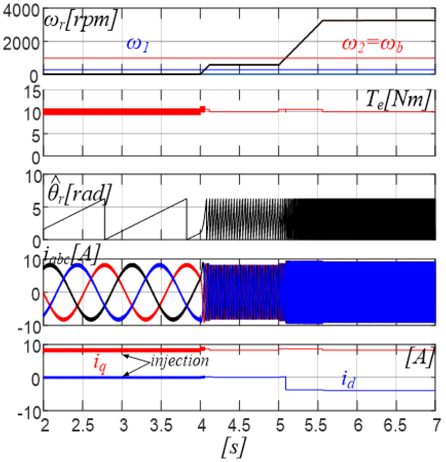
3. Sensorless Control Strategy

According to the block diagram of Figure 2, when the PMSM works in the low-speed range (ω_r ≤ ω₁), the high frequency injection sensorless technique is activated. Differently, when the PMSM works at medium and high speed range (ω₁ < ω_r ≤ ω₂), a back-EMF based estimation algorithm is exploited. Moreover, in the flux-weakening region, (ω_r > ω₂), the open winding configuration is transformed into a conventional wye one.

3.1. High Frequency Injection: 0 < ω_r < ω₁

The injection of the additional carrier signal V_hf is accomplished through the auxiliary TLI PWM (by setting I = 1 in the scheme of Figure 2), while the MLI works at low switching frequency, as shown in Figure 3. The Equation (11) can be rewritten as:

$${{\displaystyle V}}_{TLI\_i}^{*}= {{\displaystyle V}}_{TLIr\_i}^{*}+{{\displaystyle V}}_{TLIh\_i}^{*}+V_{cap\_i}+V_{hf\_i}$$

(12)

A persistent excitation V_{hf_i} is thus provided, allowing a continuous estimation of the rotor flux angle. The injected qd-axes’ high frequency voltage components are:

$$V_{qhf}= V_{hf}\cos \left({{\displaystyle \omega }}_{hf}t\right) V_{dhf}= -V_{hf}\sin \left({{\displaystyle \omega }}_{hf}t\right)$$

(13)

where V_hf and ω_hf are, respectively, the amplitude and angular frequency of the injected voltage.

In a conventional PWM-operated MLI, the peak voltage reference must be suitably reduced in order to generate the additional HF excitation. This does not happen on the considered configuration, as the HF signal is rather produced by the auxiliary TLI. Moreover, in this case, the TLI DC-Bus voltage can be easily increased during sensorless low-speed operations in order to provide the extra voltage required by HF injection, thus making the current shaping unaffected by the HF additional excitation. The interaction between the high frequency voltage and the machine saliency produces a current component at the carrier frequency containing information about the position of the rotor ${\widehat{\theta }}_r$ [17,26]. This position can be extracted through the algorithm described in Figure 4. Stator currents i^s_qds consist of the fundamental component (ω_et) and two further components at the angular frequency of the injected signal, respectively, featuring a positive (ω_hft) and a negative (2θ_r − ω_hft) sequence. The current negative sequence component contains spatial information in its phase and is proportional to the differential stator transient inductance. The current positive sequence component contains no spatial information and is proportional to the average stator transient inductance. The fundamental and the positive sequence components of the HF current vector are first isolated from the stator current by using a synchronous filter, extracting the negative sequence component. The rotor position and speed are then obtained by exploiting a heterodyne demodulation algorithm, as shown in Figure 4.

3.2. Back-EMF Estimation: ω₁ < ω_r < ω₂

Application of back-EMF-based methods to surface-mounted PMSM is quite straightforward. More complex mathematical formulations are required whenever salient machines, such as the interior PMSM (IPMSM), are considered [27,28,29,30,31]. According to the proposed approach, a saliency-based back-EMF model was developed in the stationary reference frame. Figure 5 shows the block diagram of the back-EMF estimation algorithm, where E_{qds_sal} represents the back-EMF produced by the saliency.

Observer input quantities are measured phase currents and voltages at the stator winding terminals. Phase voltages are obtained by suitably scaling the reference voltages generated by the current controllers, according to the actual DC-Bus voltage. In the considered OWPMSM configuration, the fundamental component of the phase motor voltages V_{m_i} are defined as the difference between the fundamental components of the MLI output voltages ${{\displaystyle V}}_{MLI\_i}^{*}$ and the fundamental components of the TLI output voltages.

$$V_{m\_i}={{\displaystyle V}}_{MLI\_i}^{*}-\left({{\displaystyle V}}_{TLIr\_i}^{*}+{{\displaystyle V}}_{cap\_i}^{}\right)$$

(14)

The back-EMF components are sent to a motion observer to extract the estimated rotor position [32].

3.3. Flux Weakening: ω_r > ω₂

Whenever the drive operates in the flux-weakening region, the auxiliary TLI is deactivated, and all the six switches are held in the on-state in order to obtain a wye configuration. In this condition only the MLI is active providing the current control through a step modulation of the stator voltage. As a result, the MLI is entirely charged of the current control task, as shown in Figure 6.

Although the stator voltage in this condition is distorted, the stator current is quite sinusoidal, due to the stator winding, low-pass filtering action. As in the previous case, the stator voltage fundamental component can be obtained from the current controllers, leading to a back-EMF estimation through an observer as that schematized in Figure 5.

A simulation dealing with the PMSM motor, whose data are summarized in

Table 1. OWPMSM Technical Specifications.

Rated power	2 kW	λPM	0.4 Wb
Rated torque	10.8 Nm	Ld	3.5 mH
Maximum speed	5000 rpm	Lq	3.5 mH
Pole pairs	3	Rs	1.85 Ω
Rated voltage	400 V	J	0.01 kgm2
Base speed	1000 rpm

, accomplishing a speed transient from the extreme low-speed region (ω₁ < ω_r) to the low-speed region (ω₁ < ω_r < ω₂), and then to the high speed region (ω_r > ω₂), is shown in Figure 7. At the beginning, the motor speed is 10 rpm (below ω₁ = 286 rpm) and the current injection (700 Hz) is performed to estimate the rotor position θ_e. At t = 4 s, the motor speed reference is changed from 10 rpm to 500 rpm and the back-EMF estimation technique is activated when ω_r exceeds 286 rpm. Finally, the reference speed is set to 3000 rpm in the flux-weakening area.

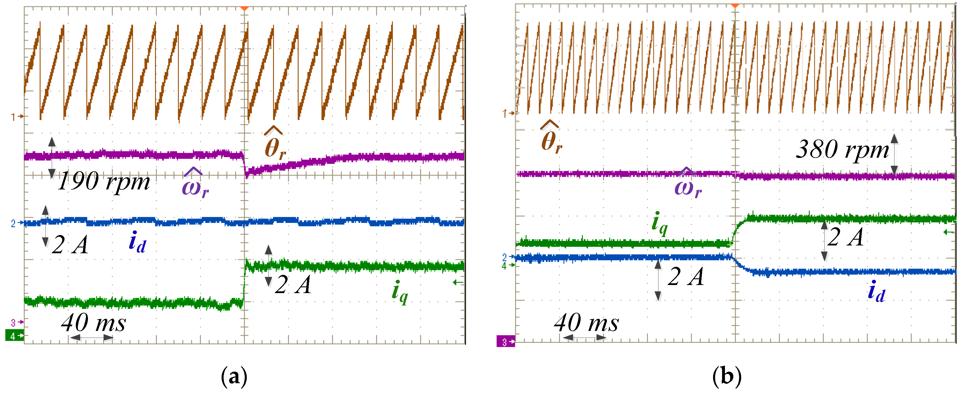
4. Performance Evaluation

Experimental tests have been carried out on a scaled system tailored around a 2 kW, three-phase, 6 poles Open-end Winding PMSM, whose technical specifications are listed in Table 1. The AHMLI system has been tested using an IGBTs 3LI Neutral Point Clamped (NPC) inverter as the main unit with V^′_DC = 300 V, and a two-level MOSFETs inverter operating at 10 kHz with a dead time of 1 μs. Power devices’ technical specifications are shown in

Table 2. IGBT STGP30H60DF Technical Specifications.

Rated voltage	600 V
Rated current	30 A
Collector-emitter saturation voltage	2 V
Turn-on switching losses	0.35 mJ
Turn-off switching losses	0.4 mJ

and

Table 3. MOSFET STW46NF30 Technical Specifications.

Rated voltage	300 V
Rated current	42 A
Static drain-source on-resistance	75 mΩ
Rise time	38 ns
Fall time	46 ns

. The TLI DC-Bus is built around a 450 µF floating capacitor, whose voltage is controlled according to (10), while the voltage across the MLI DC-Bus capacitors is kept constant by an actively controlled power supply system. Both the main and auxiliary inverter are controlled through a dSpace 1103 development control board. Sensorless rotor position estimation from HF signal injection is first investigated. Maximum possible value of the fundamental component of the TLI output voltage ${{\displaystyle V}}_{TLIh\_i}^{*}$ at half the rated load is shown in Figure 8a as a function of the rotor speed. As it is possible to observe, ${{\displaystyle V}}_{TLIh\_i}^{*}$ drops as the speed increases, because the fraction of the DC-Bus voltage required by the HF signal injection increases with the motor speed. This can be faced by suitably increasing V^″_DC. It has been shown by many authors, in particular by R.D. Lorenz, that at extreme low speed, the induced back-EMF estimation does not allow to estimate the rotor position with sufficient precision. The estimation of the rotor position is also affected by the bandwidth of the Band Pass Filters (BPF) used in the heterodyne demodulator, as shown in Figure 4. In fact, the filter time delay and attenuation decrease when increasing the difference between the fundamental frequency and the injected signal frequency, achieving a higher precision in determining the rotor position. In order to set ω₁ in the extreme low-speed range, rotor position error has been evaluated versus rotor speed. According to Figure 8b, ω₁ can be set to 285 rpm. Hence, from 285 rpm to maximum speed of 5000 rpm, a back-EMF-based estimation algorithm is exploited. In detail, from ω₁ = 285 rpm to the base speed 1000 rpm, the motor is OW configurated while, in the flux-weakening region (from 1000 rpm to 5000 rpm), the motor windings are wye connected.

A test dealing with the motor phase voltage THD, is reported in Figure 9. The THD is computed up to the 90th harmonic as function of the motor speed and V^″_DC.

The a-phase MLI output stepped voltage V_{MLIstep_a}, the a-phase TLI reference voltage ${{\displaystyle V}}_{TLI\_a}^{*}$, the a-phase motor voltage V_am and the TLI DC-Bus voltage V^″_DC are shown in Figure 10a. The TLI reference voltage ${{\displaystyle V}}_{TLI\_a}^{*}$ also includes the high frequency voltage component V_hf. Figure 10b shows the estimated rotor electrical position ${\widehat{\theta }}_{re}$, the a-phase current i_am and the qd-axes’ current components i^hf_qhf and i^hf_dhf. The a-phase current consists of the fundamental and high frequency (700 Hz) component i_hf. A zoomed view of the previous test is reported in Figure 11, highlighting the presence of the high frequency injection on the phase motor current and TLI reference voltage. Figure 12 shows the estimated mechanical speed during a 47 to −47 rpm speed reversal, the estimated rotor position ${\widehat{\theta }}_{re}$, the rotor speed error e_ωr and rotor position error e_θr with the drive operating with a 50% of rated load torque, and V^″_DC = 150 V. The rotor speed error is lower than 4.7 rpm, while the rotor position error is lower than 2 deg. Sensorless rotor position estimation based from back- EMF detection is then considered. Figure 13 shows the estimated back-EMF’s E^s_{qds_sal} and the qd-axes’ stator currents i_qd, when the motor runs at 763 rpm. Figure 14 shows the estimated rotor position, the estimated mechanical speed, the rotor speed error e_ωr, and rotor position error e_θr during a speed variation from 190 rpm to 763 rpm with a 50% of rated load torque. Figure 15 shows the qd-axes’ stator currents, the estimated rotor position, and the estimated mechanical speed during a load current variation from 2A to 4A. In detail, in Figure 15a, the rotor speed is below the base value while Figure 15b deals with field-weakening operation with wye motor winding connection. Figure 16 shows the voltages and current waveforms when the PMSM spins at 763 rpm. Note that for higher rotor speed, the TLI DC-Bus voltage can be reduced from V^′_DC/2 as in Figure 10a to V^′_DC/4 as made in the test of Figure 1.

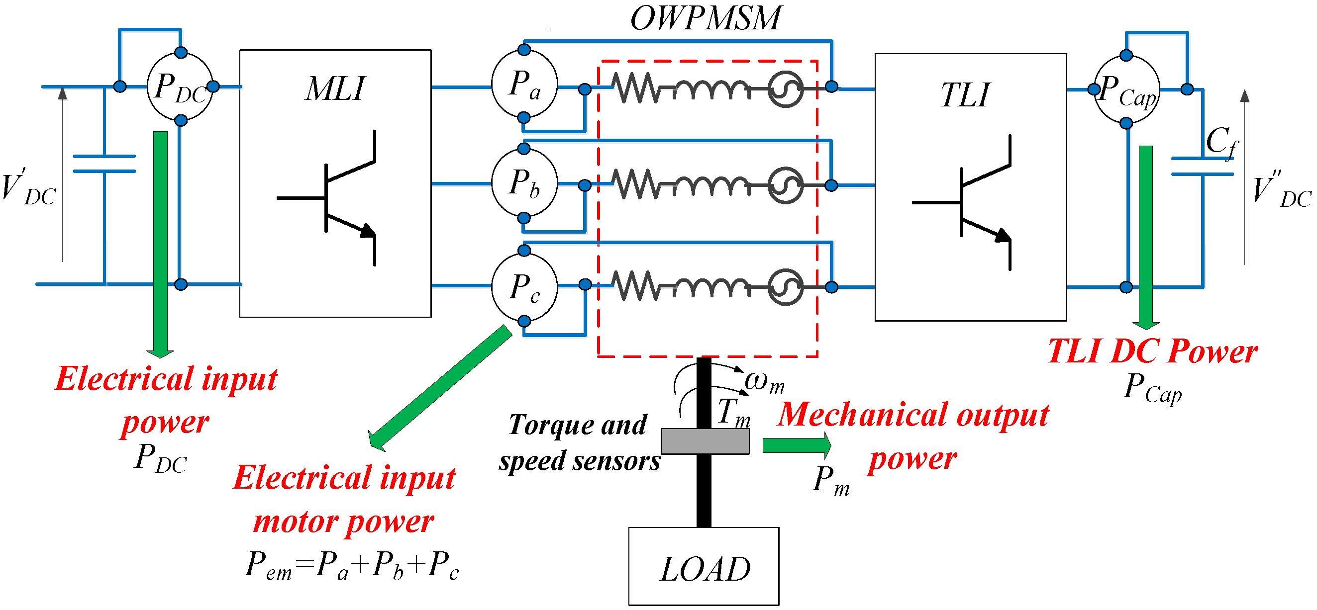
5. Power Losses Assessment

An investigation has been accomplished about the efficiency of an AHMLI-supplied OWPMSM, exploiting the proposed sensorless control approach. The MLI topology is equipped with 600 V IGBTs, while in the TLI, the 300 V MOSFETs, whose data are listed in Table 2, are used. The experimental system built for efficiency measurement is shown in Figure 17. It consists of three power analyzers placed on the DC-Bus of the MLI, on the OWPMSM, and on the DC-Bus of the TLI. Such a system detecting the input DC power P_DC, input motor power P_em, and TLI DC power P_cap is able to separately evaluate the MLI efficiency and TLI efficiency. Exploitation of modern power analyzers permits to take into account all current and voltage harmonic components in efficiency estimation. A torque sensor, connected between the motor and the mechanical load, is used to compute the motor output mechanical power P_m and efficiency. The MLI and TLI power losses can be written as:

$$P_{MLI}=P_{DC}-P_{em}=P_{MLI-cond}+P_{MLI-sw} P_{TLI}=P_{em}-P_m-P_{cap}=P_{TLI-cond}+P_{TLI-sw}$$

(15)

being P_MLI-cond, the MLI conduction losses; P_MLI-sw, the MLI switching losses; P_TLI-cond, the TLI conduction losses, and P_TLI-sw, the TLI switching losses. The power analyzer measures the total power losses, so to evaluate separately conduction losses and switching losses, the following equations are considered:

$$\begin{array}{l} P_{MLI-cond}=V_{ceon}i\delta \\ P_{MLI-sw}=0.5V_{ce}i{f}_{sw-MLI}(t_{r-IGBT}+t_{f-IGBT})\end{array}\begin{array}{l} P_{TLI-cond}=R_{DSon}{i}^2\\ P_{TLI-sw}=0.5V_{DS}i{f}_{sw-TLI}(t_{r-MOSF}+t_{f-MOSF})\end{array}$$

(16)

where V_ceon is the IGBT on-state emitter-collector voltage; δ is the duty cycle obtained by MLI step modulation; f_sw-MLI is the switching frequency of MLI; t_r-IGBT and t_f-IGBT are the rise time and fall time of the IGBTs; R_DSon is the on-state drain-source resistance of the MOSFETs; V_DS is the drain-source voltage; f_sw-TLI is the switching frequency of TLI while t_r-MOSF and t_f-MOSF are the rise time and fall time of the MOSFETs.

Obtained results have been compared with those of more conventional, sensorless controlled MLI motor drives with similar features, and equipped with the same kind of IGBT devices. Three different drive configurations have been considered for power losses’ analysis, namely: AHMLI (5LI + TLI), 5LI, and 7LI. In the last two cases (5LI and 7LI), a conventional multicarrier 10 kHz PWM is adopted in normal operations, and a step voltage modulation is exploited in flux weakening, in order to obtain straightforwardly comparable results. As shown in Figure 18, three operating conditions are considered, namely:

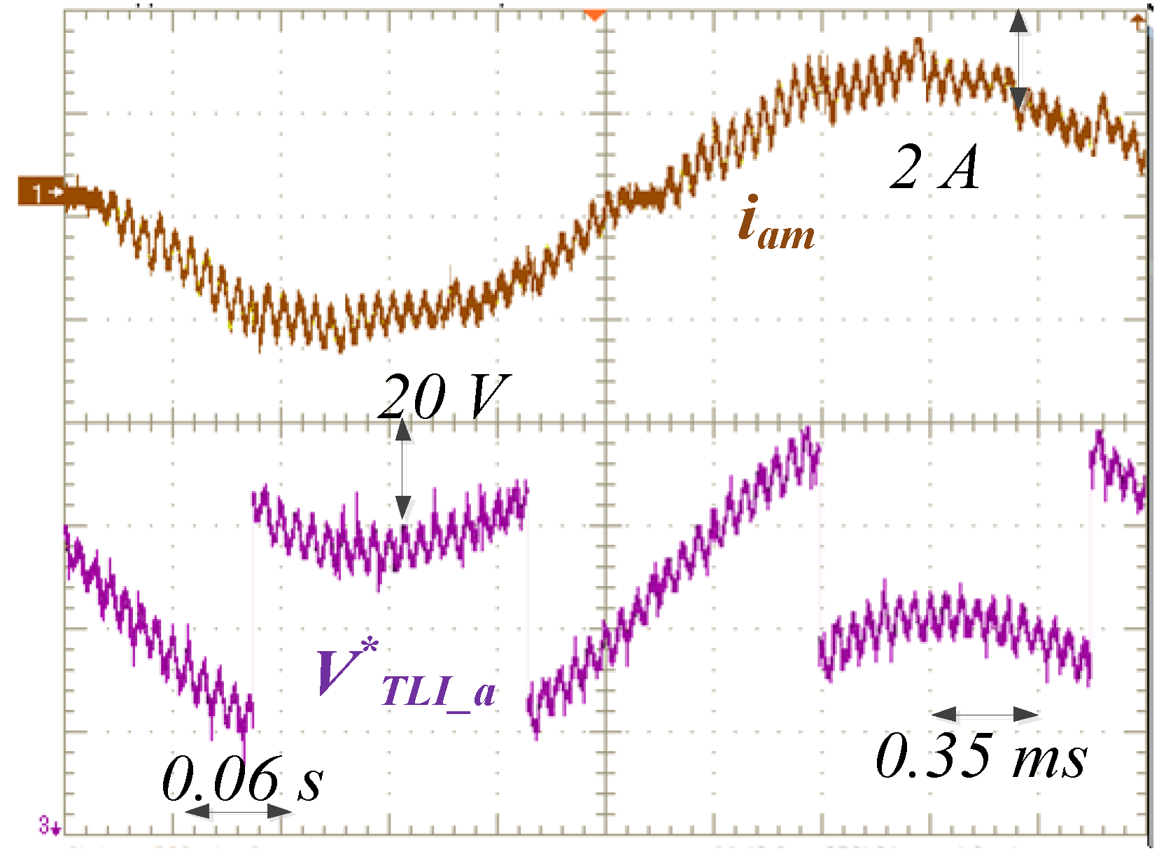
• low-speed (47 rpm) operation with HF injection and PWM voltage modulation,
• medium-speed (954 rpm) operation with back-EMF estimation and PWM voltage modulation,
• flux-weakening (2387 rpm) operations with back-EMF estimation and step voltage modulation.

Compared to the other two configurations, exploiting the AHMLI shows, in general, lower total switching power losses. In fact, the PWM voltage modulation is accomplished by the auxiliary TLI, which, in comparison with conventional PWM-operated MLI is equipped with faster power MOSFET devices, and works at a lower DC-Bus voltage. The advantage is particularly noticeable on low-speed operation, due to the additional workload required by the HF signal injection. Lower motor losses are also obtained, as more clean current and voltage waveforms are produced [32]. Conduction power losses are quite equivalent among AHMLI and MLI configurations, as the multilevel inverters are equipped with the same devices. However, the MLI of the AHMLI configuration is always step-operated, thus, it can be equipped with slower power devices featuring lower conduction losses, leading to a further efficiency improvement. In flux-weakening operations, the AHMLI configuration is marginally less efficient, due to TLI conduction losses. In this case, in fact, the wye configuration is obtained by holding on all the six switches.

6. Conclusions

A self-sensing control approach has been proposed for a particular type of multilevel inverter motor drive. In such a kind of system, an Open-end Winding AC Motor is fed on one side by a main multilevel inverter, and on the other side, by an auxiliary two-level inverter. Current control is shared between the two inverters, whose operational modes are selected in order to take full advantage from their specific features. According to the proposed approach, a high frequency injection technique is exploited to estimate the rotor position at low speed. Differently from more conventional drive configurations, the HF signal injection does not affect the operation of the MLI, as it is accomplished through the auxiliary TLI. Moreover, as the last is equipped with a floating bus capacitor, its DC-Bus voltage can be easily increased in low-speed operations, in order to provide the extra voltage required by HF injection. Finally, additional switching power losses caused by HF signal excitation are quite lower than in equivalent multilevel motor drives. At medium and high speed, a back-EMF-based rotor position estimation technique is used. In this case, a greater efficiency is obtained in comparison with conventional multilevel inverters. In fact, the MLI is step-operated, thus minimizing switching power losses. The PWM voltage modulation is accomplished by the auxiliary TLI, which in comparison with conventional PWM-operated MLI is equipped with faster power devices, and works at a lower DC-Bus voltage. The paper deals with a PM synchronous motor drive, however, the proposed technique can be also used on induction motor drives. It provides a viable alternative on pumps, fans, compressors, extruders, mixers, and conveyor drives in hostile environment, or where a wide-speed range is required with rated load torque and soft-starting, in mining, transports, cement, and metal processing plants, petrochemical, and gas industries.

References

1. Kouro, S.; Malinowski, M.; Gopakumar, K.; Pou, J.; Franquelo, L.G.; Wu, B.; Rodriguez, J.; Perez, M.A.; Leon, J.I. Recent Advances and Industrial Applications of Multilevel Converters. IEEE Trans. Ind. Electron. 2010, 57, 2553–2580. [Google Scholar] [CrossRef]
2. Wang, M.; Hu, Y.; Zhao, W.; Wang, Y.; Chen, G. Application of modular multilevel converter in medium voltage high power permanent magnet synchronous generator wind energy conversion systems. IET Renew. Power Gener. 2010, 25, 1786–1799. [Google Scholar] [CrossRef]
3. Hagiwara, M.; Nishimura, K.; Akagi, H. A Medium-Voltage Motor Drive with a Modular Multilevel PWM Inverter. IEEE Trans. Power Electron. 2016, 10, 324–833. [Google Scholar]
4. Kaarthik, R.S.; Gopakumar, K.; Mathey, J.; Underland, T. Medium Voltage Drive for Induction Machine with Multilevel Dodeca-gon Voltage Space Vectors with Symmetric Triangles. IEEE Trans. Ind. Electron. 2014, 62, 79–87. [Google Scholar] [CrossRef]
5. Nabae, A.; Takahashi, I.; Akagi, H. A New Neutral-Point-Clamped PWM Inverter. IEEE Trans. Ind. Appl. 1981, IA-17, 518–523. [Google Scholar] [CrossRef]
6. Bhagwat, P.M.; Stefanovic, V.R. Generalized structure of a multi-level PWM inverter. IEEE Trans. Ind. Appl. 1983, IA-19, 1057–1069. [Google Scholar] [CrossRef]
7. Lai, J.-S.; Peng, F.Z. Multi-level converters-A new breed of power converters. IEEE Trans. Ind. Appl. 1996, 32, 509–517. [Google Scholar]
8. Okazaki, Y.; Matsui, H.; Muhoro, M.M.; Hagiwara, M.; Akagi, H. Capacitor-Voltage Balancing for a Modular Multilevel DSCC Inverter Driving a Medium-Voltage Synchronous Motor. IEEE Trans. Ind. Appl. 2016, 52, 4074–4083. [Google Scholar] [CrossRef]
9. Cacciato, M.; Consoli, A.; Scarcella, G.; Testa, A. Reduction of common-mode currents in PWM inverter motor drives. In Proceedings of the 1997 IEEE Industry Applications Conference 32nd IAS Annual Meeting, New Orleans, LA, USA, 5–9 October 1997; Volume 1, pp. 707–714. [Google Scholar]
10. Mohapatra, K.K.; Gopakumar, K.; Somasekhar, V.T.; Umanand, L. A harmonic elimination and suppression scheme for an open-end winding induction motor drive. IEEE Trans. Ind. Electron. 2003, 50, 1187–1198. [Google Scholar] [CrossRef]
11. Foti, S.; Testa, A.; Scelba, G.; Cacciato, M.; Scarcella, G.; De Caro, S.; Scimone, T. Overvoltage mitigation in open-end winding AC motor drives. In Proceedings of the 2015 International Conference on Renewable Energy Research and Applications (ICRERA), Palermo, Italy, 22–25 November 2015; pp. 238–245. [Google Scholar]
12. Scelba, G.; Scarcella, G.; Foti, S.; Testa, A.; De Caro, S.; Scimone, T. An Open-end Winding approach to the design of multi-level multi-motor drives. In Proceedings of the IECON 2016—42nd Annual Conference of the IEEE Industrial Electronics Society, Florence, Italy, 23–26 October 2016; pp. 5026–5032. [Google Scholar]
13. Edpuganti, A.; Rathore, A.K. New Optimal Pulse Width Modulation for Single DC-Link Dual-Inverter Fed Open-End Stator Winding Induction Motor Drive. IEEE Trans. Power Electron. 2015, 30, 4386–4393. [Google Scholar] [CrossRef]
14. Somasekhar, V.T.; Gopakumar, K.; Bajiu, M.R.; Mohapatra, K.K.; Umanand, L. A multilevel inverter system for an inductor motor with open-end windings. IEEE Trans. Ind. Electron. 2015, 52, 824–836. [Google Scholar] [CrossRef] [Green Version]
15. Srinivas, S.; Sekhar, K.R. Theoretical and Experimental Analysis for Current in a Dual-Inverter-Fed Open-End Winding Induction Motor Drive with Reduced Switching PWM. IEEE Trans. Ind. Electron. 2012, 60, 4318–4328. [Google Scholar] [CrossRef]
16. Ge, B.; Peng, F.Z.; de Almeida, A.T.; Abu-Rub, H. An Effective Control Technique for Medium-Voltage High Power Induction Motor Fed by Cascaded Neutral Point Clamped Inverter. IEEE Trans. Ind. Electron. 2010, 57, 2659–2668. [Google Scholar]
17. Alves, J.A.; Torri, P.; da Cunha, G. Medium Voltage Industrial Variable Speed Drives. Pulse 2009, 6, 8. [Google Scholar]
18. Scarcella, G.; Scelba, G.; Testa, A. High performance sensorless controls based on HF excitation: A viable solution for future AC motor drives? In Proceedings of the 2015 IEEE Workshop on Electrical Machines Design, Control and Diagnosis (WEMDCD), Torino, Italy, 26–27 March 2015; pp. 178–187. [Google Scholar]
19. Consoli, A.; Scarcella, G.; Testa, A. Slip-Frequency Detection for Indirect Field-Oriented Control Drives. IEEE Trans. Ind. Appl. 2004, 40, 194–201. [Google Scholar] [CrossRef]
20. Wang, S.; Lu, Z. Study on Wide Range Robust Speed Sensorless Control of Medium Voltage Induction Motor. In Proceedings of the Twenty-Fifth Annual IEEE Applied Power Electronics Conference and Exposition (APEC), Palm Springs, CA, USA, 21–25 February 2010; pp. 1542–1546. [Google Scholar]
21. Shukla, R.D.; Tripathi, R.K. Speed-sensorless voltage & frequency control in autonomous DFIG based wind energy systems. In Proceedings of the 2014 Australasian Universities Power Engineering Conference (AUPEC), Perth, Australia, 28 September–1 October 2014; pp. 1–6. [Google Scholar]
22. Jansen, P.L.; Lorenz, R.D. A physically insightful approach to the design and accuracy assessment of flux observers for field oriented induction machine drives. IEEE Trans. Ind. Appl. 1994, 30, 101–110. [Google Scholar] [CrossRef] [Green Version]
23. Degner, M.W.; Lorenz, R.D. Using Multiple Saliencies for the Estimation of Flux, Position, and Velocity in AC Machines. IEEE Trans. Ind. Appl. 1998, 34, 1097–1104. [Google Scholar] [CrossRef] [Green Version]
24. Lin, T.C.; Zhu, Z.Q. Sensorless Operation Capability of Surface-Mounted Permanent-Magnet Machine Based on High-Frequency Signal Injection Methods. IEEE Trans. Ind. Appl. 2015, 51, 2161–2171. [Google Scholar] [CrossRef]
25. Foti, S.; Testa, A.; De Caro, S.; Scimone, T.; Pulvirenti, M. Rotor Flux Position Correction and Parameters Estimation on Sen-sorless Multiple Induction Motors Drives. IEEE Trans. Ind. Appl. 2019, 55, 3759–3769. [Google Scholar] [CrossRef]
26. Fot, S.; Testa, A.; De Caro, S.; Scimone, T.; Scelba, G.; Scarcella, G. Rotor Time Constant Identification on Sensorless Induction Motor Drives by low Frequency Signal Injection. In Proceedings of the 2018 IEEE 9th International Symposium on Sensorless Control for Electrical Drives (SLED), Helsinki, Finland, 13–14 September 2018; pp. 150–155. [Google Scholar]
27. Kshirsagar, P.; Krishnan, R. Sensorless Control of Permanent Magnet Motors Operating at Low Switching Frequency for Climate Control Systems. In Proceedings of the 3rd IEEE International Symposium on Sensorless Control for Electrical Drives (SLED 2012), Milwaukee, WI, USA, 21–22 September 2012; pp. 1–8. [Google Scholar]
28. Uddin, N.; Rashid, M.M.; Rubaiyat, M.; Hossain, B.; Salam, S.M.; Nithe, N.A. Comparison of position sensorless control based back-EMF estimators in PMSM. In Proceedings of the 18th International Conference on Computer and Information Technology (ICCIT), Dhaka, Bangladesh, 21–23 December 2015; pp. 5–10. [Google Scholar]
29. Halder, S.; Agarwal, P.; Srivastava, S.P. MTPA based Sensorless Control of PMSM using position and speed estimation by Back-EMF method. In Proceedings of the IEEE 6th International Conference on Power Systems (ICPS), New Delhi, India, 4–6 March 2016; pp. 1–4. [Google Scholar]
30. Johnson, P.M.; Bai, K.; Ding, X. Back-EMF-Based Sensorless Control Using the Hijacker Algorithm for Full Speed Range of the Motor Drive in Electrified Automobile Systems. IEEE Trans. Transp. Electrif. 2015, 1, 126–137. [Google Scholar] [CrossRef]
31. Lin, F.-J.; Hung, Y.-C.; Chang, J.-K. Sensorless IPMSM drive system using saliency back-EMF-based observer with MTPA control. In Proceedings of the International Conference on Electrical Machines and Systems (ICEMS), Hangzhou, China, 22–25 October 2014; pp. 3539–3545. [Google Scholar]
32. De Caro, S.; Foti, S.; Scimone, T.; Testa, A.; Cacciato, M.; Scarcella, G.; Scelba, G. THD and efficiency improvement in multi-level inverters through an open end winding configuration. In Proceedings of the IEEE Energy Conversion Congress and Exposition (ECCE), Milwaukee, WI, USA, 18–22 September 2016; pp. 1–7. [Google Scholar]
33. Foti, S.; Testa, A.; Scelba, G.; De Caro, S.; Cacciato, M.; Scarcella, G.; Scimone, T. An Open End Winding Motor Approach to miti-gate the phase voltage distortion on Multi-Level Inverters. IEEE Trans. Power Electron. 2018, 33, 2404–2416. [Google Scholar] [CrossRef]
34. Scelba, G.; Scarcella, G.; Foti, S.; De Caro, S.; Testa, A. Self-sensing control of open-end winding PMSMs fed by an asymmetrical hybrid multilevel inverter. In Proceedings of the IEEE International Symposium on Sensorless Control for Electrical Drives (SLED), Catania, Italy, 18–19 September 2017; pp. 165–172. [Google Scholar] [CrossRef]
Figure 1. An AHMLI converter supplying an OWPMSM.
Energies 15 03166 g001
Figure 2. Block diagram of the AHMLI sensorless current control system.
Energies 15 03166 g002
Figure 3. MLI step modulation and TLI PWM on the a-phase.
Energies 15 03166 g003
Figure 4. HF_injection and heterodyne demodulation.
Energies 15 03166 g004
Figure 5. Back-EMF estimation in the stationary reference frame in the Medium-High speed range.
Energies 15 03166 g005
Figure 6. AHMLI current control system in Flux Weakening.
Energies 15 03166 g006
Figure 7. Speed transients from 10 rpm (extreme low-speed region) to 500 rpm (low-speed region), and from 500 rpm to 3000 rpm (flux-weakening region). Te = 10 Nm.
Energies 15 03166 g007
Figure 8. (a) Maximum possible value of V*TLI_abc vs. rotor speed at 50% of the rated torque. The HF signal injection is switched off beyond 285 rpm. (b) Rotor Position error versus rotor speed.
Energies 15 03166 g008
Figure 9. Phase voltage THD vs. rotor speed for two values of VDC at 50% of the rated torque. The HF signal injection is switched off beyond 285 rpm.
Energies 15 03166 g009
Figure 10. HF injection-based estimation technique: ωr = 47 rpm, load torque Tr = 50% rated, VDC = 300 V, VDC = 150 V, Vhf = 30 V and fhf = 700 Hz: VMLI_stepa, V T L I _ a * , Vam, and TLI DC-Bus voltage VDC (a), θ ^ r e , iam, ihfqdhf (b).
Energies 15 03166 g010
Figure 11. HF injection-based estimation technique: ωr = 47 rpm, load torque Tr = 50% rated, VDC = 300 V, VDC = 150 V, Vhf = 30 V, and fhf = 700 Hz: i a m , V T L I _ a * .
Energies 15 03166 g011
Figure 12. HF injection-based estimation technique: speed step from 47 rpm to −47 rpm, load torque Tr = 50% rated, VDC = 300 V and VDC = VDC/4: ω ^ r, θ ^ r e , eωr, and eθr.
Energies 15 03166 g012
Figure 13. Back-EMF-based estimation: ωr = 763 rpm, load torque Tr = 50% rated, VDC = 300 V, VDC = 50 V: Esqd_sal, and isqd in stationary reference frame.
Energies 15 03166 g013
Figure 14. Back-EMF-based estimation technique, speed transient 190 rpm to 763 rpm, load torque Tr = 50% rated: estimated θ ^ re, ω ^ r, and actual rotor position θ r e , eωr, and eθr.
Energies 15 03166 g014
Figure 15. Back-EMF-based estimation technique, load torque transient from 25% to 50% rated (a) ωr = 763 rpm; (b) flux weakening ωr = 1526 rpm. θ ^ re, ω ^ r, iqd.
Energies 15 03166 g015
Figure 16. Back-EMF-based estimation, ωr = 763 rpm, load torque Tr = 50%, rated torque, VDC = 300 V, V′′DC = 75 V: iam, V T L I _ a * , and TLI DC-Bus voltage V′′DC.
Energies 15 03166 g016
Figure 17. Test bench for power losses’ analysis.
Energies 15 03166 g017
Figure 18. Inverter power losses—MLI conduction losses PMLI-cond, MLI switching losses PMLI-sw, TLI conduction losses PTLI-cond, TLI switching losses PTLI-sw: (a) AHMLI—2387 rpm, flux weakening; (b) AHMLI—954 rpm, back-EMF estimation; (c) AHMLI—47 rpm, HF injection; (d) 5LI—2387 rpm, flux weakening; (e) 5LI—954 rpm, back-EMF estimation; (f) 5LI—47 rpm, HF injection; (g) 7LI—2387 rpm, flux weakening; (h) 7LI—954 rpm, back-EMF estimation; (i) 7LI—47 rpm, HF injection.
Energies 15 03166 g018