Modeling of Large-Scale Thermal Power Plants for Performance Prediction in Deep Peak Shaving

Abstract

To integrate more renewable energy into the power grid, large-scale thermal power plants have to extend their operating ranges and participating in deep peak shaving. In order to improve the thermal economy of large-scale thermal power plants participating in deep peak shaving, and to determine the performance of a thermal system under different conditions, a method of modeling for the performance prediction of large-scale thermal power plants in deep peak shaving is proposed. In the algorithm design of the model, a three-layer iterative cycle logic is constructed, and the coupling relationship between the parameters of the thermal system is analyzed from the mechanism level. All of the steam water parameters and the correction values of the flow rate at all levels of the system after the parameter disturbance are obtained. The algorithm can simulate the response of a thermal power plant under load variation and operation parameter variation. Compare the error between the data given by the prediction model and the test, the accuracy of the proposed prediction model is verified. When the unit participates in deep peak shaving, the prediction model is used to analyze the relative deviation of the unit thermal efficiency caused by cycle parameters and energy efficiency of equipment. It provides a date basis for the performance evaluation and multi-parameter coupling optimization. The research results can be used to determine the operation mode and equipment transformation scheme.

1. Introduction

Large-scale thermal power plants are the main power producers in China. With China’s increasing emphasis on energy conservation and emissions reduction, increasing the proportion of renewable energy, reducing thermal power generation represent the new trends of development in energy production and consumption [1,2,3,4,5]. At the same time, due to the unstable characteristics of renewable energy power generation, the function of thermal power generation units in the energy supply system should also be adjusted accordingly, from being the major supplier of electricity to maintaining stable load and providing standby load. Therefore, thermal power units are required to participate in deep peak shaving. The participation of coal-fired generating units in deep peak shaving can greatly raise the compatibility of the energy supply system. It plays an important role in promoting the transformation of energy structure [6,7,8,9].

Denmark aims to achieve power generation without fossil fuels by 2050 [10]. An important requirement in order to achieve this goal is that thermal power units have a high degree of flexibility. Germany’s energy structure is being adjusted in order to develop the renewable energy will account for more than 50% of the total power generation in the future. At the same time, this requires large-scale thermal power plants participate in deep peak shaving to balance the load fluctuation [11].

In summary, thermal power units are relied upon when participating in deep peak shaving in order to realize the reformation of the energy structure [12,13]. At the same time, large-scale thermal power plants participate in deep peak shaving will affect the overall thermal economy of the thermal power plants, and the performance indicators will change greatly compared with those of the design overview [14,15,16,17,18].

Çetin et al. [19] compared and discussed the power generation efficiency of three different thermal power sources. Clay and Mathias [20] analyzed the thermal economy of subcritical 173 MW coal-fired power plants. Kumar et al. [21] conducted a thermal economic analysis of a coal-fired power plant and determined the energy loss distribution. Oyedepo et al. [22] completed the thermal performance analysis of steam turbine power plants with reheaters. The result of thermodynamic theoretical analysis shows that the thermal efficiency of system is improved when the number of closed feedwater heaters is increased from 1 to 10. Through thermodynamic analysis, Wang et al. [23] found that the use of double reheat technology can improve the efficiency of coal-fired power plants. Zhou et al. [24] analyzed a 1000 MW coal-fired power plant with the technology of supercritical carbon dioxide. Their energy analysis showed that compared with traditional steam power plants, s-co2 power plants have a higher average heat absorption temperature and overall energy efficiency. In addition, some scholars [25,26,27,28] have evaluated the performance of steam power plants with different capacities and determined the system energy efficiency.

It can be seen from the literature review that a large number of studies have evaluated the performance of thermal power-generating units under design conditions (rated load). It can be found that the performance index of thermal power units is affected by three types of factors: external load and ambient temperature (circulating water temperature and its corresponding circulating water flow and unit exhaust pressure); cycle parameters (main steam parameters, etc.); and the energy efficiency of the main and auxiliary equipment (cylinder efficiency and heater terminal temperature difference). When calculating the performance index of a thermal power unit, in addition to the main steam, extraction parameters, reheat steam parameters, heater effluent and hydrophobic parameters are also required. In the real-time calculation and replay calculation of historical data, real-time measurement data and historical record data can be used. The measurement method can be considered as a replacement for thermal system mechanism analysis in order to obtain the system state parameters, as the latter method can only carry out historical analysis and post evaluation.

More specifically, the performance evaluation of thermal power units is hindered by the following problems: (1) when thermal power units participate in deep peak shaving, the unit deviates from the design condition and works in partial load operation. At present, although the units can measure the values of various parameters through measuring points and calculate their performance indicators, it is difficult to obtain data from predictive calculations. As a result, the thermal economy of the units cannot be predicted and analyzed. (2) In thermal power units, the main steam pressure and exhaust steam pressure not only have a separate impact on the system evaluation index, but also have a coupling relationship with one another. This parameter coupling also makes it difficult to establish a performance prediction model for thermal power units. (3) Due to the operation optimization calculation demand when thermal power units participate in deep peak shaving, it is difficult to calculate the system evaluation index in the case of parameter disturbance under a partial load. Establishing a performance prediction model and studying the performance change laws of units constitute major problems that must be solved in the performance evaluation and system optimization of thermal power units participating in deep peak shaving.

There are no studies in the literature that focus on predicting the thermal economy of a unit under parameter disturbance when the unit participates in deep peak shaving. In order to solve the above problems, a performance prediction model of thermal power units under a full load (30~100%) is proposed. Moreover, the following interesting outcomes, as the main achievements of this study, are briefly summarized as follows:

(1)

A modeling method for the performance prediction of large-scale thermal power plants during deep peak shaving is proposed;

(2)

Parameter coupling is fully considered in the model’s construction, and three-layer iterative logic is adopted in the algorithm design of the model. In the innermost layer, a mechanism analysis of the condenser’s heat transfer characteristics is used as the constraint for the end of the iterative calculation of exhaust pressure. In the middle layer, the Flugel formula is used as the constraint for the end of the iteration calculation of the extraction pressure at each extraction point. In the outermost layer, the power balance equation is used as the constraint for the end of the iterative calculation of the main steam flow. Through the model design of the three-layer iterative cycle mode, the extraction coefficient and condensation coefficient can be used as the coupling point; synchronous iterative calculations of exhaust flow, exhaust pressure and exhaust enthalpy are realized; and the mechanisms of the coupling relationships between various parameters can be analyzed. The corrected values of all steam and water parameters of the system and the flow of groups at all levels after parameter disturbance are thereby obtained;

(3)

The accuracy of the model is verified by the measured data of the power plant;

(4)

The influence of different types of disturbance parameters on the performance of thermal power units when these units participate in deep peak shaving are reported. In addition, the change laws of unit performance indexes when the cycle parameters (main steam and reheat steam parameters) are disturbed are predicted, as well as the change laws of unit performance indexes when the energy efficiency parameters of the main and auxiliary equipment (high-pressure cylinder efficiency and end difference) are disturbed.

The remainder of this paper is organized as follows: Section 1 introduces the cur-rent situation regarding the performance evaluation of thermal power units, and dis-cusses the difficulties of performance prediction when thermal power units participate in deep peak shaving. A modeling method for the performance prediction of large-scale thermal power plants during deep peak shaving is proposed in Section 2. Section 3 provides the simulation calculations used for model verification and the variation laws of unit performance under different types of parameter disturbances. Taking the deviation of the heat rate as the analysis index, the performance of a 300 MW unit is analyzed and evaluated using the prediction model; the changes in the system’s thermal economy under different loads and different disturbance parameters are analyzed; and the performance change curves under different loads and different disturbance parameters are given, in order to realize the performance prediction of the unit when participating in deep peak shaving. Our conclusions are drawn in Section 4.

When the unit participates in deep peak shaving, the prediction model is used to analyze the relative deviation of the unit thermal efficiency caused by cycle parameters and energy efficiency of equipment, obtain performance change curve. It provides a date basis for the performance evaluation and multi-parameter coupling optimization. The research results can be used to determine the operation mode and equipment transformation scheme, make it operate economically, and finally reduce the energy consumption of the power plant.

2. Materials and Methods

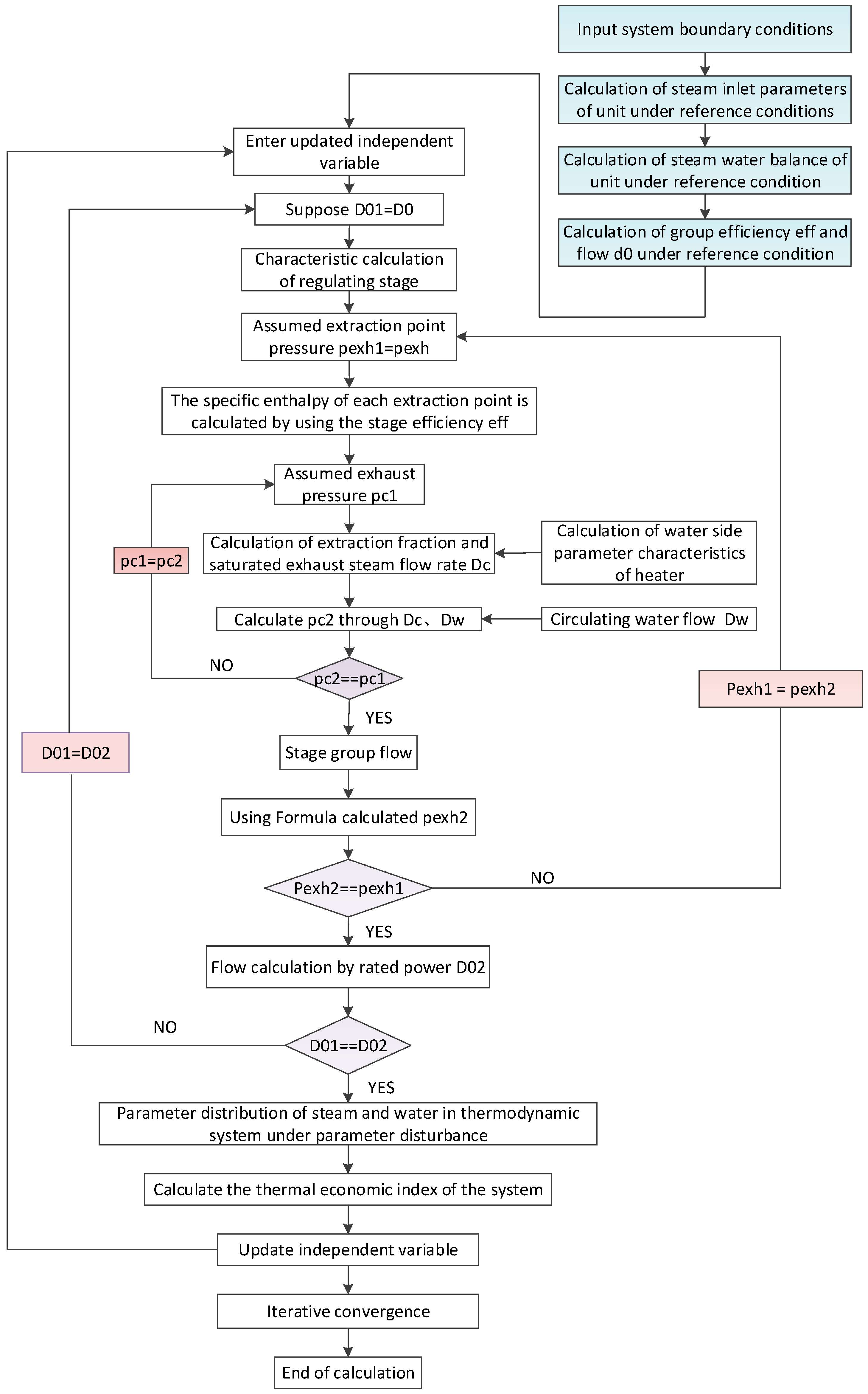
2.1. Performance Prediction Modeling

When the unit participates in deep peak shaving, the operating conditions of the unit is affected by three types of factors: external load and ambient temperature (circulating water temperature and its corresponding circulating water flow and unit exhaust pressure); cycle parameters (main steam parameters, etc.); and the energy efficiency of the main and auxiliary equipment (cylinder efficiency and heater terminal temperature difference). The starting point of the prediction model is to redetermine the new steam expansion process line of the steam turbine when the input disturbance of the thermal system changes. Once the new steam state line is determined, the pressure of various heaters, the enthalpy of the inlet and outlet temperature of condensate, and the extraction flow of each extraction coefficient can be determined accordingly.

Logical flowchart of the performance prediction model is shown in Figure 1.

When the unit is disturbed by factors, the parameters causing the change of working conditions are substituted into the calculation model, according to the characteristic model of flow passage, characteristic model of heater and characteristic model of condenser, calculate the variation of steam extraction at all levels. Determine the system state parameters synchronously. Parameter coupling is fully considered in the model’s construction, and three-layer iterative logic is adopted in the algorithm design of the model. A mechanism analysis of the condenser’s heat transfer characteristics, the Flugel formula and power balance equation are used as the constraint for the end of the iterative calculation of exhaust pressure, the extraction pressure at each extraction point and the main steam flow. Through the model design of the three-layer iterative cycle mode, the extraction coefficient and condensation coefficient can be used as the coupling point; synchronous iterative calculations of exhaust flow, exhaust pressure and exhaust enthalpy are realized; and the mechanisms of the coupling relationships between various parameters can be analyzed. The corrected values of all steam and water parameters of the system and the flow of groups at all levels after parameter disturbance are thereby obtained.

2.2. Characteristic Model of Flow Passage

2.2.1. Calculation of Extraction Pressure

According to the relationship between the stage group flow in the flow passage section and the changes in parameters before and after the stage group [29,30,31], the formula to calculate the stage group flow can be obtained as follows:

$$\frac{D_{j1}}{D_{j0}}=\frac{{\beta }_1}{\beta }\cdot \frac{p_{j1}}{p_{j0}}\sqrt{\frac{T_{j0}}{T_{j1}}}=\sqrt{\frac{{\left(1-{\epsilon }_{nc}\right)}^2-{\left({\epsilon }_{n1}-{\epsilon }_{nc}\right)}^2}{{\left(1-{\epsilon }_c\right)}^2-{\left({\epsilon }_n-{\epsilon }_{nc}\right)}^2}}\cdot \frac{p_{j1}}{p_{j0}}\sqrt{\frac{T_{j0}}{T_{j1}}}$$

(1)

where $D_j$ is the through flow rate of the j stage group, (t/j); β is the Pengtaimen coefficient; ${\epsilon }_n$ is the pressure ratio before and after the stage group;${\epsilon }_c$ is the critical pressure ratio before and after the stage group;$p_{j }$ is the pre-stage pressure of the stage group j, MPa; and $T_j$ is the thermodynamic temperature of the stage group j, K.

In the subscript, “0” indicates the parameters under reference working conditions, and “1” indicates the parameters under variable working conditions.

When the stage group is in the critical state, or there are many stages in the stage group and the critical pressure ratio is very small, Formula (1) of each stage extraction pressure in the flow passage section can be changed as follows:

$$\frac{D_{j1}}{D_{j0}}=\sqrt{\frac{p_{j1}^2-p_{\left(j-1\right)1}^2}{p_{j0}^2-p_{\left(j-1\right)0}^2}}\cdot \sqrt{\frac{T_{j0}}{T_{j1}}}$$

(2)

where P_{(j − 1)} is the extraction pressure of the (j − 1) stage, MPa.

If the stage from steam extraction to the low-pressure cylinder is regarded as a stage group, and the stage group is in a critical state before and after the change in working conditions, then at this time the post-stage pressure is very small compared with the pre-stage pressure, and the flow of the stage group is related only to the pre-stage pressure. According to Formula (2), and ignoring the post-stage pressure, we can obtain

$$\frac{D_{j1}}{D_{j0}}=\frac{p_{j1}}{p_{j0}}\cdot \sqrt{\frac{T_{j0}}{T_{j1}}}$$

(3)

That is, the calculation formula of the extraction pressure in the flow passage section is

$$p_{j1}=\frac{p_{j0}}{D_{j0}\cdot \sqrt{T_{j0}}}\cdot \sqrt{T_{j1}}\cdot D_{j1}$$

(4)

When calculating the steam exhaust of the HP cylinder, it is necessary to first determine the steam pressure at the inlet of the IP cylinder (reheater outlet). According to Formula (4), we can obtain the following:

$$p_{rh1}=\frac{p_{rh0}}{D_{rh0}\cdot \sqrt{T_{rh0}}}\cdot \sqrt{T_{rh1}}\cdot D_{rh1}$$

(5)

where $D_{rh}$ is the steam flow at the inlet of reheater outlet, t/h; $p_{rh}$ is the steam pressure at the reheater outlet, MPa; and $T_{rh}$ is the steam thermodynamic temperature at the reheater outlet, K.

In general, the pressure loss of steam passing through the reheater is directly proportional to the steam flow passing through the reheater. Therefore, the actual pressure loss under variable conditions can be calculated from the corresponding parameters under reference conditions as follows:

$$\Delta p_{rh}=\frac{\Delta p_{rh0}}{D_{rh0}\cdot \sqrt{T_{rh0}}}\cdot \sqrt{T_{rh1}}\cdot D_{rh1}$$

(6)

According to the pressure of steam at the outlet of the reheater and the pressure loss of steam passing through the reheater, it can be concluded that the exhaust pressure of the HP cylinder is

$$p_{Ho}=p_{rh}+\Delta p_{rh}$$

(7)

When calculating the extraction pressure of the last stage, when the unit is in a critical or supercritical state, Formula (4) can be used. When the last stage group is in a subcritical state, the post-stage pressure of the last stage group cannot be ignored, compared with the pre-stage pressure; according to Formula (2), the extraction pressure of the last stage can be obtained as follows:

$$\frac{D_{11}}{D_{10}}=\sqrt{\frac{p_{11}^2-p_{c1}^2}{p_{10}^2-p_{c0}^2}}\cdot \sqrt{\frac{T_{10}}{T_{11}}}$$

(8)

The exhaust pressure of the steam turbine P_c can be obtained according to the condensing flow and the condenser characteristic mode.

2.2.2. Stage Group Efficiency Calculation

• Efficiency calculation of the regulating stage

Steam passing through the regulating valve occurs by a throttling process, and so the enthalpy of the steam flow behind each regulating valve is equal to the enthalpy of the main steam. At the same time, the ideal enthalpy drop of each regulating valve can be obtained by the steam thermodynamic parameters in front of each regulating valve and the isentropic expansion in the pressure after the regulating stage. Through the ideal enthalpy drop of each regulating valve, the speed ratio of each regulating valve can be calculated, and the effective enthalpy drop of each regulating valve can be calculated according to the characteristic curve of the regulating stage. After the effective enthalpy drop of each regulating valve is multiplied by the respective flow and then divided by the total flow, the effective enthalpy drop of the regulating stage can be obtained [32,33,34].

The efficiency of the regulating stage is the effective enthalpy drop of the regulating stage divided by the ideal enthalpy drop of the main steam.

2.

Intermediate stage efficiency calculation

The stage group from the second stage to the last stage is referred to as the intermediate stage group. The pressure in front of the intermediate stage group changes in direct proportion to the flow, so the pressure ratio of the intermediate stage remains unchanged when the working conditions change. The steam temperature before and after each stage in the intermediate stage group is essentially unchanged, so the speed ratio and ideal enthalpy drop of the stage group are almost unchanged. It can therefore be assumed that the efficiency of the stage group does not change.

3.

Final stage efficiency calculation

In the actual production process, the exhaust steam pressure loss is considered to be approximately zero. That is, it is assumed that the exhaust pressure of the last stage of the steam turbine is equal to the pressure of the condenser. Therefore, the exhaust pressure of the last stage is obtained by using the variable condition of the condenser. Based on the design data, the law of the variation in the relative internal efficiency of the last stage with the pressure ratio of the last stage is obtained, which fits the relationship between the pressure ratio of the last stage and the efficiency of the last stage.

The final stage efficiency can be calculated with the following formula:

$${\eta }_i=-2.988\times {\epsilon }^2+1.42\times \epsilon +0.725$$

(9)

where ε is the last stage pressure ratio.

In the last stage’s characteristic calculation, the exhaust pressure $p_c$ of the steam turbine is obtained by using the condenser characteristics. Meanwhile, according to the relationship between the efficiency and the pressure ratio of the last stage, the exhaust enthalpy $h_c$ of the last stage can be obtained by drawing the thermal process line for this stage.

The exhaust enthalpy calculated from Equation (9) is shown in

Table 1. Verification of final exhaust enthalpy.

Load	50%	60%	75%	85%
Exhaust enthalpy test value (kJ/kg)	2369.18	2361.68	2377.57	2357.88
Exhaust enthalpy calculated value (kJ/kg)	2368.54	2360.04	2378.02	2359.62
Error (%)	−0.03	−0.07	0.02	0.07

. According to the calculation results in Table 1, the accuracy of the results is within 0.1%, which meets the actual requirements of the project. The calculation results prove this method is reliable, by comparing the calculated value with that of the test.

2.2.3. Extraction Enthalpy and Temperature Calculation

The relative internal efficiency of the stage group is defined as

$${\eta }_{j~\left(j-1\right)}=\frac{h_j-h_{j-1}}{h_j-h_{ja}}$$

(10)

where ${\eta }_{j~\left(j-1\right)}$ is the relative internal efficiency of the stage group between the j stage extraction port and the j − 1 stage extraction port; $h_{j }$ is the inlet steam enthalpy of the stage group, kJ/kg; $h_{j-1}$ is the outlet steam enthalpy of the stage group, kJ/kg; and $h_{ja}$ is the enthalpy of isentropic expansion from the pre-stage state point to the post-stage pressure state point, kJ/kg.

According to Formula (10), the enthalpy value of steam extraction at all stages can be calculated as follows:

$$h_{j-1}=h_j-\left(h_j-h_{ja}\right)\cdot {\eta }_{jr}$$

(11)

According to the extraction pressure and extraction enthalpy calculated above, the extraction temperature can be obtained through the steam property function, with the following calculation formula:

$$t_j=f\left(p_j,h_j\right)$$

(12)

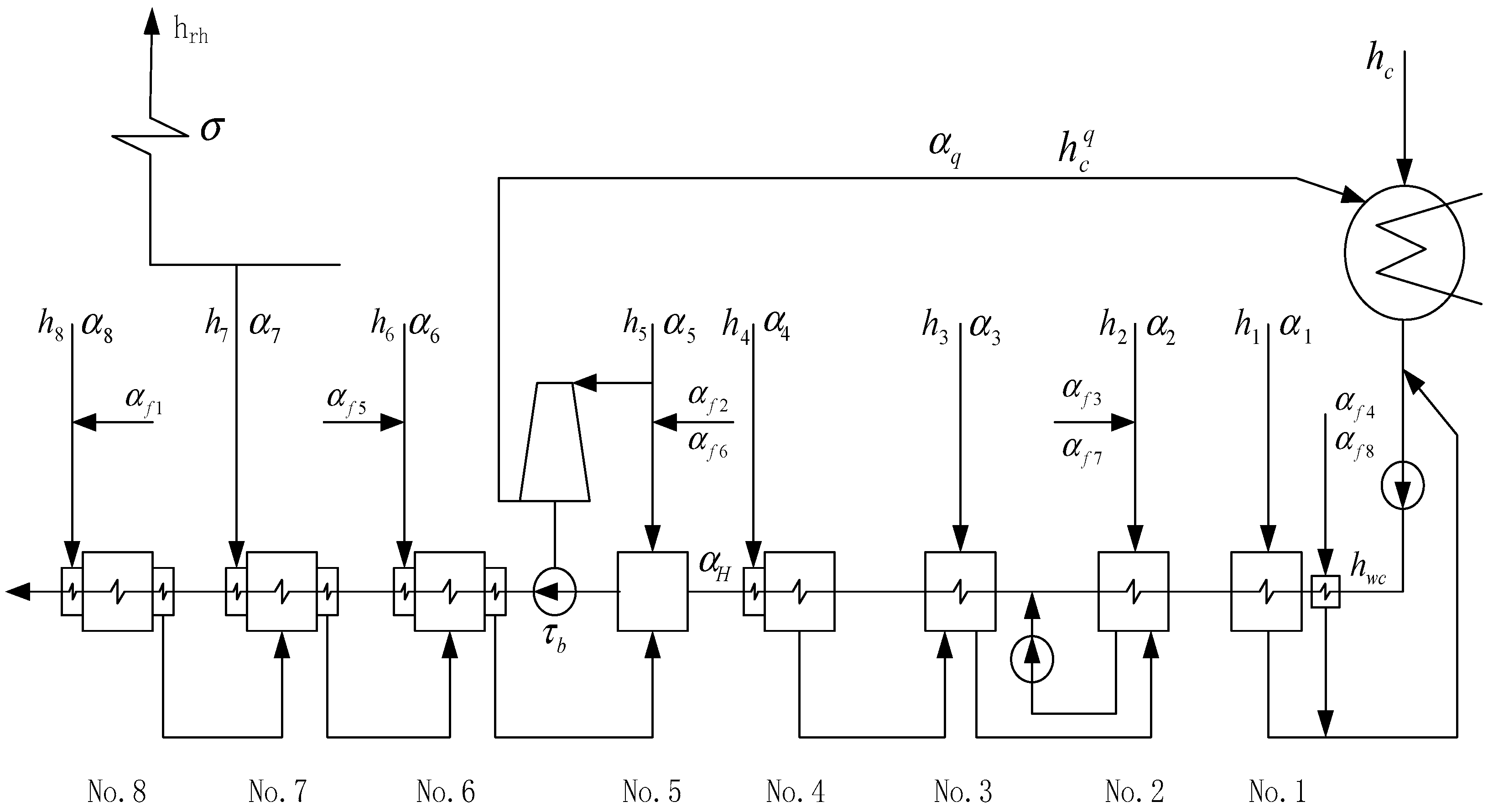
2.3. Characteristic Model of the Heater

2.3.1. Change in Inlet and Outlet Parameters

For any stage heater in the thermal system, the outlet water temperature $t_{w,j}$, the specific enthalpy $h_{w,j}$, the inlet water temperature $t_{w,j}^{\prime }$ and the inlet water specific enthalpy $h_{w,j}^{’}$ can be calculated in the following order:

$$p_{s,j}=p_j-\Delta p_j$$

(13)

$$t_{s,j}=f\left(p_{s,j}\right)$$

(14)

$$t_{w,j}=t_{s,j}-\sigma t$$

(15)

$$h_{w,j}=f\left(p_{w,j},t_{w,j}\right)$$

(16)

$$t_{w,j}^{’}=t_{w,j+1}$$

(17)

$$h_{w,j}^{’}=h_{w,j+1}$$

(18)

where $p_{s,j}$ is the saturation pressure in the heater after the working conditions change, MPa; $t_{s,j}$ is the saturation temperature in the heater after the working conditions change, °C; and $\sigma t$ is the upper terminal temperature difference in the heater, given constant, °C.

Formula (16) uses the principle of terminal difference invariance before and after the change in working conditions.

2.3.2. Extraction Enthalpy and Temperature Calculation

For a heater without a drain cooler, the specific enthalpy of drain water $h_{d,j}$ is equal to the specific enthalpy of saturated water under the heater $\mathrm{pressure} h_{s,j}$:

$$h_{d,j}=h_{s,j}$$

(19)

The heater inlet difference can also be expressed in the form of specific enthalpy:

$$\delta h_1=h_{d,j}-h_{w,j}^{’}$$

(20)

Because the pressure change at the steam and water sides of the heater is very small, $\delta h_1$ can also be regarded as a constant under variable working conditions. Therefore, the specific enthalpy of drain water $h_{d,j}$ after variable working conditions can be calculated directly with $\delta h_1$ = constant (the original working conditions are given). The $h_{d,j}$ after changing the working conditions is as follows:

$$h_{d,j}=h_{w,j}^{’}+\delta h_1$$

(21)

2.4. Characteristic Model of the Condenser

The condenser and circulating water system are important components of the thermal system. When the input parameters of thermal system change, the pressure of the condenser also change. It is therefore necessary to simulate the characteristics of the condenser to determine the condenser pressure after the input changes. Condenser pressure is affected by exhaust steam flow, exhaust steam enthalpy, circulating water flow and circulating water inlet temperature. A change in each parameter changes the condenser pressure.

2.4.1. Condenser Pressure Calculation

Many factors affect condenser condensation pressure in the actual process, including the circulating water inlet water temperature, the circulating water pump operation mode, unit load, etc. The purpose of studying the condenser variable operating conditions is to determine the variation law of the condenser condensation pressure under these influencing factors. The saturation temperature corresponding to the condenser pressure is approximately equal to the steam condensation temperature in the condenser’s main condensation area [35,36,37,38]. The steam condensation temperature in the main condensation zone at a certain cooling area is:

$$t_s=t_{w1}+\Delta t+\delta t$$

(22)

where t_s is the saturation temperature of the exhaust (°C); $t_{w1}$ is the circulating water inlet temperature (°C); $\Delta t$ is the temperature rise in the circulating water (°C); and $\delta t$ is the condenser’s terminal temperature difference (°C).

The circulating water temperature rise $\Delta t$ can be obtained from the heat balance between the heat release of the exhaust steam and the heat absorption of the circulating water:

$$\Delta t=\frac{D_c\cdot \left(h_c-h_{c\prime }\right)}{D_w\cdot c_w}=\frac{\left(h_c-h_{c\prime }\right)}{c_w}\cdot \frac{1}{m}=\frac{2177}{4.187\cdot m}\approx \frac{520}{m}$$

(23)

where $D_c$ is the exhaust volume into the condenser (t/h); $D_w$ is the circulating water flow (t/h); $c_w$ is the specific heat capacity of the circulating cooling water (kJ/(kg·K)); h_c − h_c′ is the latent heat of vaporization when 1 kg of exhaust vapor condenses in the condenser, 2177 (kJ/kg); and $m=D_w/D_c$ is the cooling multiplier of the condenser.

The condenser heat transfer terminal temperature difference is $\delta t$, derived from the heat transfer equation:

$$\delta t=\frac{\Delta t}{\exp (\frac{K_c\cdot F_c}{D_w\cdot c_p})-1}$$

(24)

where $F_c$ is the heat transfer area of the condenser (m²) and $K_c$ is the condenser heat transfer coefficient ($\mathrm{kJ}/{\mathrm{m}}^2\cdot \mathrm{h}\cdot \mathrm{K}$).

From Equations (22)–(24), the condenser condensation pressure can be finally determined under variable working conditions. From these equations, it can be seen that the heat transfer terminal temperature difference $\delta t$ is affected by $K_c$, $F_c$, $D_c$ and $D_w$. For a particular condenser, the area $F_c$ is a fixed value. Therefore, the main factors influencing the heat transfer differential $\delta t$ are the overall heat transfer coefficient $K_c$, the amount of circulating water $D_w$ and the turbine discharge $D_c$.

2.4.2. Determination Method of the Overall Heat Transfer Coefficient of the Condenser

The overall heat transfer coefficient K_c is generally calculated based on empirical formulas. One of these formulas, derived by the Behrman formula (BTИ), is as follows:

$$K_c=14650\cdot \phi \cdot {\phi }_w\cdot {\phi }_t\cdot {\phi }_z\cdot {\phi }_d$$

(25)

$${\phi }_w={\left(\frac{1.1\cdot c_w}{\sqrt[4]{d_1}}\right)}^{0.12\cdot \phi \cdot \left(1+1.5\cdot t_{w1}\right)}$$

(26)

$${\phi }_t=1-\frac{0.42\cdot \sqrt{\phi }}{1000}\cdot {\left(35-t_{w1}\right)}^2$$

(27)

$${\phi }_z=1+\frac{Z-2}{10}\cdot \left(1-\frac{t_{w1}}{35}\right)$$

(28)

where φ is the cleanliness factor. For open water supply systems, φ = 0.8~0.85; for closed water supply systems, when the water is changed frequently, φ = 0.75~0.8; and when the cooling water is not clean, φ = 0.6~0.75. φ_w is the correction coefficient for the cooling water flow rate and pipe diameter; c_w is the flow rate of the cooling water in the pipe (m/s), generally selected as 1.5~2.5 (m/s); d₁ is the inner diameter of the cooling water pipe (mm); φ_t is the correction coefficient of the cooling water inlet temperature; φ_z is the correction coefficient of the cooling water flow number Z; φ_d is the correction coefficient of the condenser per area of steam load, d_c.

3. Results with Analysis

3.1. Model Validation

The performance prediction model is verified using the test data of a 300 MW unit. The thermodynamic system diagram of the unit is shown in Figure 2.

The main steam enthalpy of the unit h₀ is 3435.8 kj/kg, the enthalpy of reheat steam h_rh is 3566.0 kj/kg, the enthalpy of exhaust steam h_c is 2394.4 kj/kg, the heat absorption of reheat σ is 493.9 kj/kg, the steam consumption share of the small steam turbine α_q is 0.043173, and the feed water enthalpy rise τ_b is 27.7 kJ/kg. There are nine auxiliary steams in total, of which the first to fourth auxiliary steams are generated before reheating the cold section. The other thermal parameters of the unit are shown in

Table 2. Unit thermal parameters.

Number	Heater Parameters					Auxiliary Steam Parameters
	hj	hwj	hdj	qj	αfk	hfk	qfk
	kJ/kg	kJ/kg	kJ/kg	kJ/kg	/	kJ/kg	kJ/kg
1	2604.4	220.9	232.9	2465.1	0.006006	3383.7	2310.1
2	2725.8	375.2	387.3	2504.9	0.0082827	3319.6	2693.7
3	2932.1	532.5	540.6	2391.5	0.0015956	3151.9	2931.0
4	3050.6	625.9	625.6	2425.0	0.00024491	3435.7	3296.4
5	3153.0	697.0	-	2527.1	0.00027072	3508.6	2760.2
6	3331.6	835.3	748.4	2583.2	0.0010685	3565.9	2940
7	3072.1	1038.5	862.6	2209.5	0.0014263	3445.2	3224.3
8	3155.4	1145.9	1073.6	2081.8	0.0009401	1581.4	1442.1

.

The test data were collected using the IMP (isolated measurement pods) system in a power plant of the China Huadian Corporation. For each working condition, the stability time is 1 h, the collection time is 1 h and the collection interval is 5 min. Finally, the value of each parameter is taken as the average value of all data points after excluding bad data points.

The 90%, 80% and 60% load conditions are selected for calculation and verification. The extraction pressure and exhaust pressure of the steam turbine are important parameters reflecting the turbine’s state, and the performance indexes of the unit are correlated with the extraction pressure. Therefore, the load rate, unit efficiency, extraction pressure and exhaust pressure of the original working condition and the predicted working condition are listed in

Table 3. Performance prediction model validation.

	Load Rate	Pel (MW)	p0 (MPa)	p8 (MPa)	p7 (MPa)	p6 (MPa)	p5 (MPa)	p4 (MPa)	p3 (MPa)	p2 (MPa)	p1 (MPa)	pc (kPa)	ηi
TestData	100%	299.9	16.71	6.052	3.674	1.704	0.945	0.547	0.281	0.135	0.095	9.169	0.414
	90%	269.6	16.69	5.322	3.319	1.538	0.854	0.494	0.255	0.132	0.096	8.650	0.411
	80%	239.6	16.79	4.751	2.930	1.351	0.748	0.433	0.224	0.125	0.094	6.899	0.411
	70%	209.7	16.79	4.184	2.596	1.193	0.659	0.381	0.198	0.121	0.094	7.691	0.408
	60%	179.9	10.29	3.609	2.225	1.022	0.577	0.332	0.173	0.117	0.094	5.968	0.407
	50%	150.0	10.78	3.012	1.879	0.859	0.482	0.277	0.145	0.112	0.095	6.414	0.402
Prediction Data	90%	270.1	16.70	5.352	3.401	1.553	0.855	0.505	0.260	0.135	0.098	8.890	0.411
	Error (%)	0.2	0.1	0.6	2.5	1.0	0.1	2.2	2.1	2.6	2.6	2.8	−0.1
	80%	240.2	16.75	4.851	2.981	1.332	0.768	0.422	0.234	0.121	0.097	6.651	0.411
	Error (%)	0.2	−0.2	2.1	1.7	−1.4	2.7	−2.6	4.6	−3.4	2.8	−3.6	0.05
	60%	180.1	10.43	3.622	2.238	1.051	0.598	0.321	0.178	0.119	0.095	6.138	0.406
	Error (%)	0.1	1.3	0.4	0.6	2.8	3.7	−3.2	3.1	2.0	0.7	2.9	−0.2

. It can be seen from Table 2 that the error between the data given by the prediction model and the corresponding working conditions in the test is very small; the maximum relative error is generally less than ±5%, and most of the relative errors are within ±1%. The relative error of the unit thermal efficiency, calculated according to the prediction model, is within ±0.2%. The calculation results show that the prediction model can be verified by the actual unit test data, with high accuracy.

3.2. Simulation of Performance Prediction Model under Parameter Disturbance

When the unit participates in deep peak shaving, a prediction model is used to analyze the influence of the deviation from various disturbance factors in the unit, and the variation in the unit work and the relative deviation of the unit thermal efficiency caused by the deviation in various factors are calculated.

The rated load of the unit is 300 MW (100% load) for a unit participating in deep peak shaving, and the 90%, 80%, 75%, 50%, 40% and 30% load conditions are selected for calculation; the minimum load of the unit is 90 MW (30% load). The disturbance factors include the main steam pressure, main steam temperature, reheat steam temperature, heater terminal temperature difference, and high-pressure cylinder efficiency.

Based on the above-mentioned analysis model, the thermal economy indexes of the unit under variable power loads and operating parameters can be obtained.

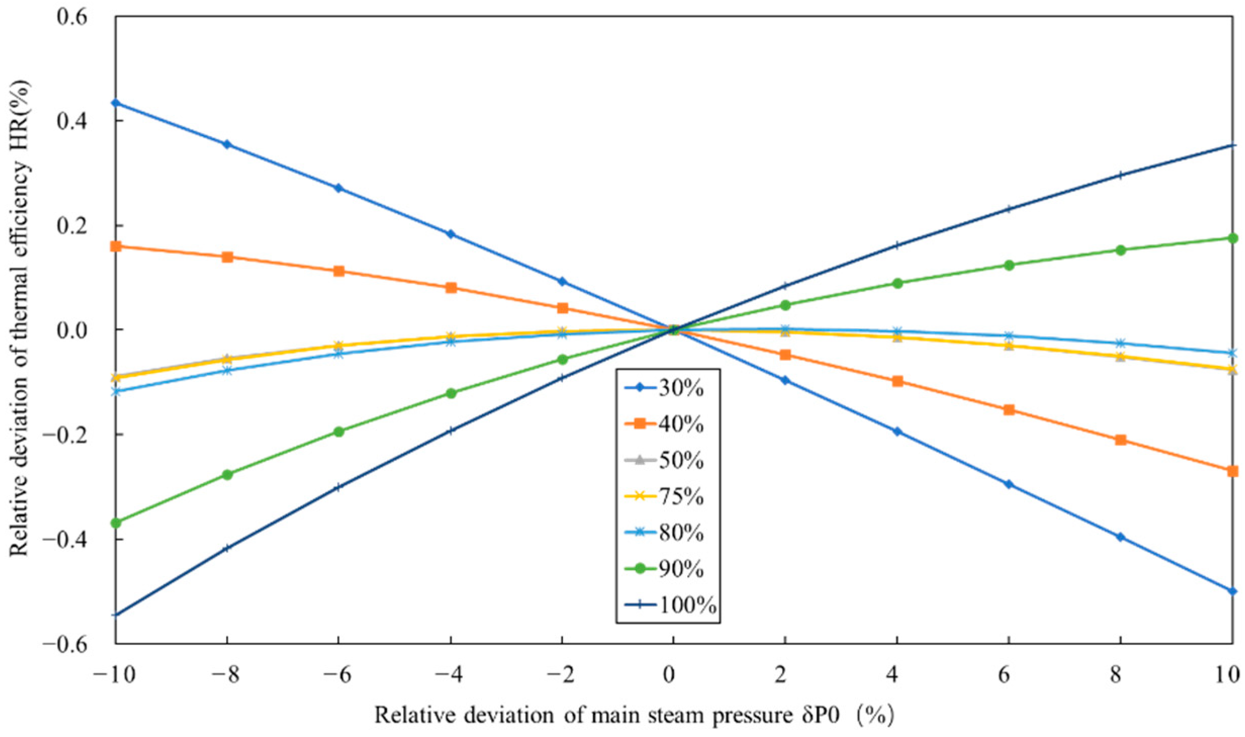
3.2.1. Main Steam Pressure Disturbances

The main steam pressure is based on the optimal sliding pressure in a typical season, and the disturbance range is −10% to 10%, with an interval of 2%.

Figure 3 shows the variation in the relative deviation of thermal efficiency with the disturbance of the main steam pressure under different output power loads. For a unit at its rated load, the unit efficiency increases with the increase in the main steam pressure: if the main steam pressure increases by 10%, then the unit thermal efficiency increases by 0.353%, or if the main steam pressure decreases by 10%, then the unit thermal efficiency decreases by 0.545%.

For a unit participating in deep peak shaving, when the main steam pressure increases compared with the reference working condition, the unit thermal efficiency decreases with the decrease in unit load; when the main steam pressure decreases compared with the reference working condition, the unit thermal efficiency increases with the decrease in unit load. When the unit is at 30% load, if the main steam pressure increases by 10%, then the unit thermal efficiency decreases by 0.499%, or if the main steam pressure decreases by 10%, then the unit thermal efficiency increases by 0.434%.

3.2.2. Main Steam Temperature Disturbances

The reference value of the main steam temperature is 540 °C and the disturbance range is −10 °C to 10 °C, with an interval of 2 °C.

Figure 4 shows the variation in the relative deviation of thermal efficiency with the disturbance of the main steam temperature under different output power loads. For a unit at its rated load, the unit thermal efficiency increases with the increase in the main steam temperature: if the main steam temperature increases by 10 °C, then the unit thermal efficiency increases by 0.253%, or if the main steam temperature decreases by 10 °C, then the unit thermal efficiency decreases by 0.258%.

For a unit participating in deep peak shaving, the change tendency is almost the same for different output power loads. When the unit is at 30% load, if the main steam temperature increases by 10 °C, then the unit thermal efficiency increases by 0.228%, or if the main steam temperature decreases by 10 °C, then the unit thermal efficiency decreases by 0.232%.

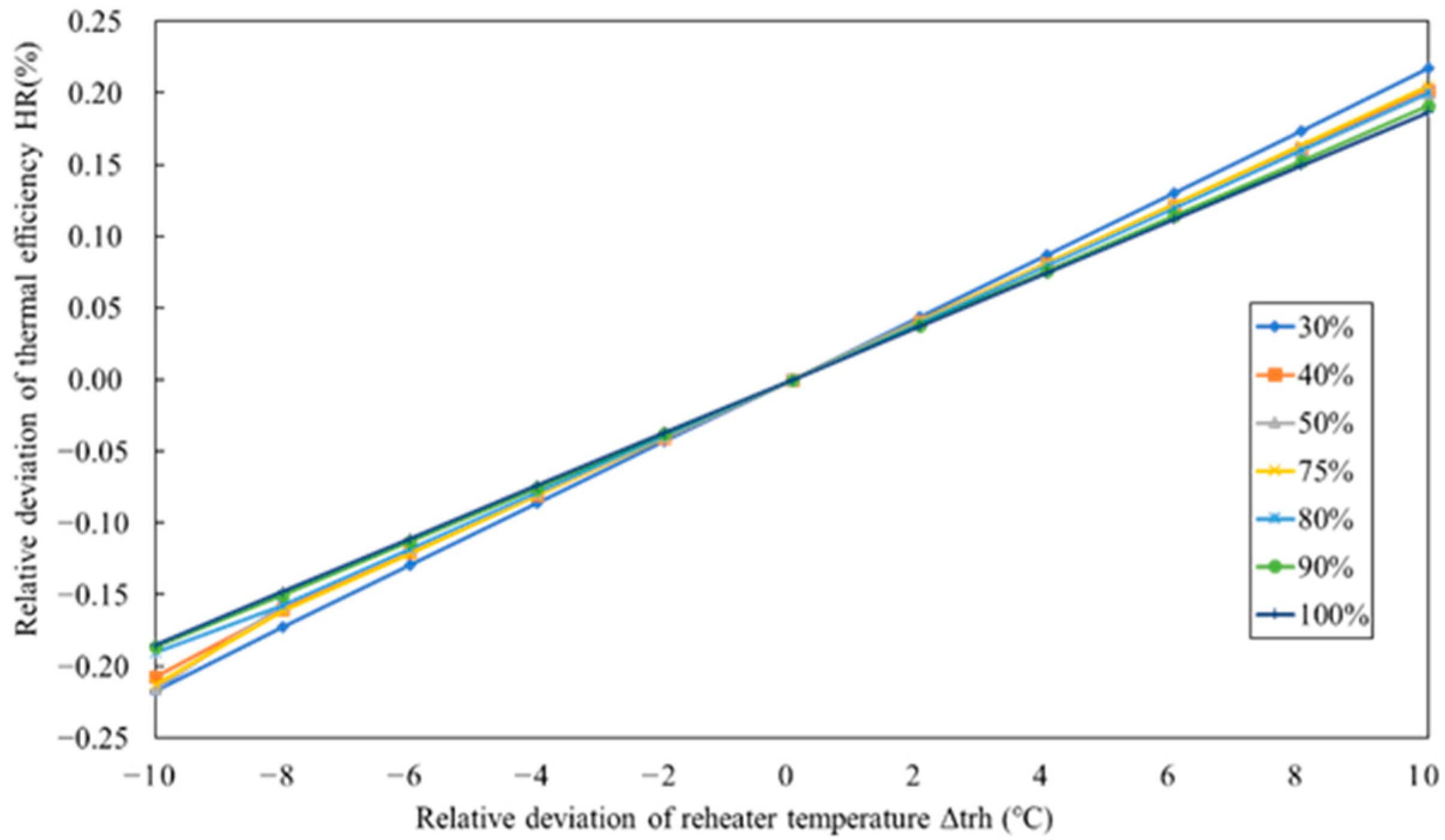
3.2.3. Reheated Steam Temperature Disturbances

The reference value of the reheated steam temperature is 540 °C and the disturbance range is −10 °C to 10 °C, with an interval of 2 °C.

Figure 5 shows the variation in the relative deviation of thermal efficiency with reheated steam temperature disturbance under different output power loads. For a unit at its rated load, the unit thermal efficiency increases with the increase in reheated steam temperature: if the reheated steam temperature increases by 10 °C, then the unit thermal efficiency increases by 0.187%, or if the reheated steam temperature decreases by 10 °C, then the unit thermal efficiency decreases by 0.185%.

For a unit participating in deep peak shaving, the change tendency is almost the same for different output power loads. When the unit is at 30% load, if the reheated steam temperature increases by 10 °C, then the unit thermal efficiency increases by 0.217%, or if the reheated steam temperature decreases by 10 °C, then the unit thermal efficiency decreases by 0.216%.

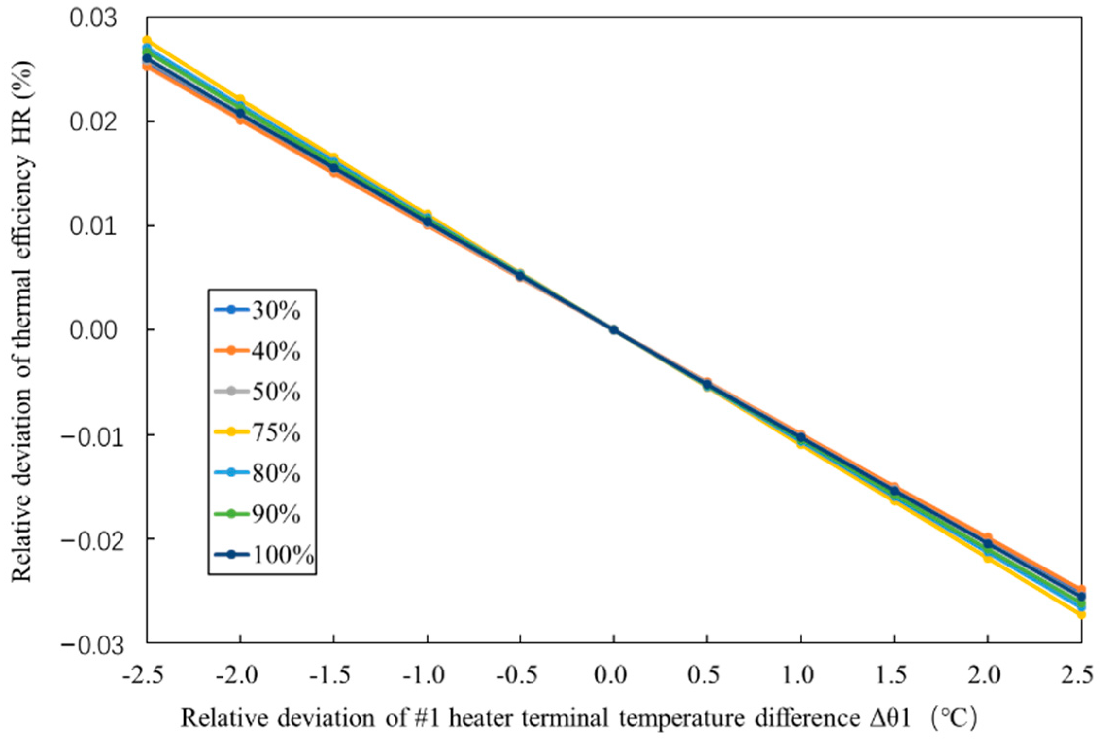
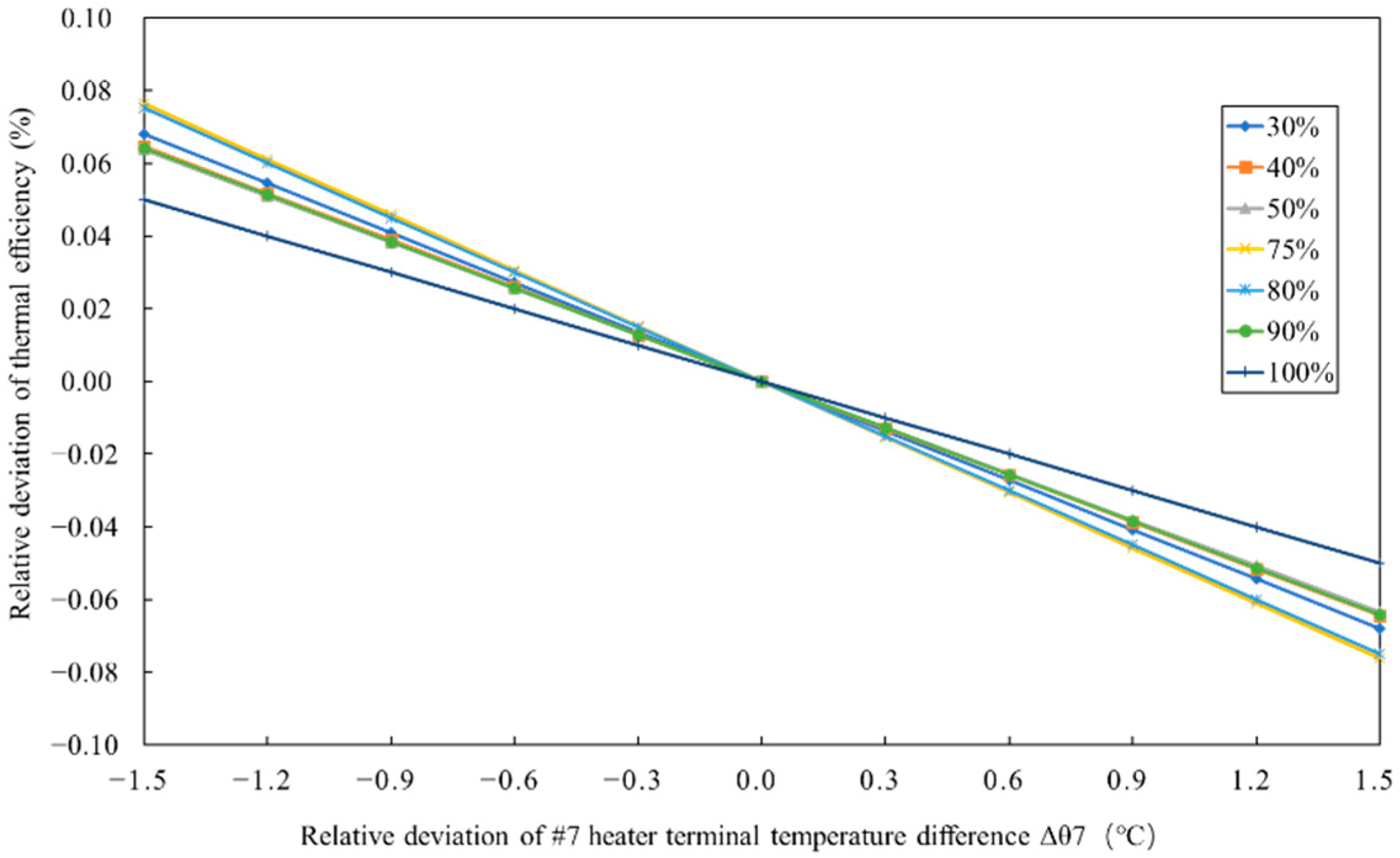
3.2.4. Heater Terminal Temperature Difference Disturbance

Generally speaking, the changes in the terminal temperature in the first and last heater stages have the greatest influence on the efficiency of the unit. Therefore, the terminal temperature differences in the #1 and #7 heaters are selected for study. The base value of the #1 heater terminal temperature difference is 3 °C, and the disturbance range is −2.5 °C~2.5 °C, with an interval of 0.5 °C. The reference value of the #7 heater terminal temperature difference is 2 °C, and the disturbance range is −1.5 °C~1.5 °C, with an interval of 0.3 °C.

Figure 6 and Figure 7 show the variation in the relative deviation of thermal efficiency with a disturbance in the heater terminal temperature difference under different output power loads. For a unit at its rated load, the unit thermal efficiency decreases with the increase in heater terminal temperature difference: the #1 heater terminal temperature difference increases by 1.5 °C, and the unit thermal efficiency decreases by 0.0154%; the #7 heater terminal temperature difference increases by 1.5 °C, and the unit thermal efficiency decreases by 0.05%; the #1 heater terminal temperature difference decreases by 1.5 °C, and the unit thermal efficiency increases by 0.0156%, and the #7 heater terminal temperature difference decreases by 1.5 °C, and the unit thermal efficiency increases by 0.05%.

For a unit participating in deep peak shaving, the change tendency is almost the same for different output power loads. When the unit is at 30% load, the #1 heater terminal temperature difference increases by 1.5 °C, and the unit thermal efficiency decreases by 0.0152%; the #7 heater terminal temperature difference increases by 1.5 °C, and the unit thermal efficiency decreases by 0.0679%; the #1 heater terminal temperature difference decreases by 1.5 °C, and the unit thermal efficiency increases by 0.0154%; and the #7 heater terminal temperature difference decreases by 1.5 °C, and the unit thermal efficiency increases by 0.0682%.

It is found from the above analysis that the #7 heater terminal temperature difference has a greater impact on the unit thermal efficiency than the #1 heater terminal temperature difference.

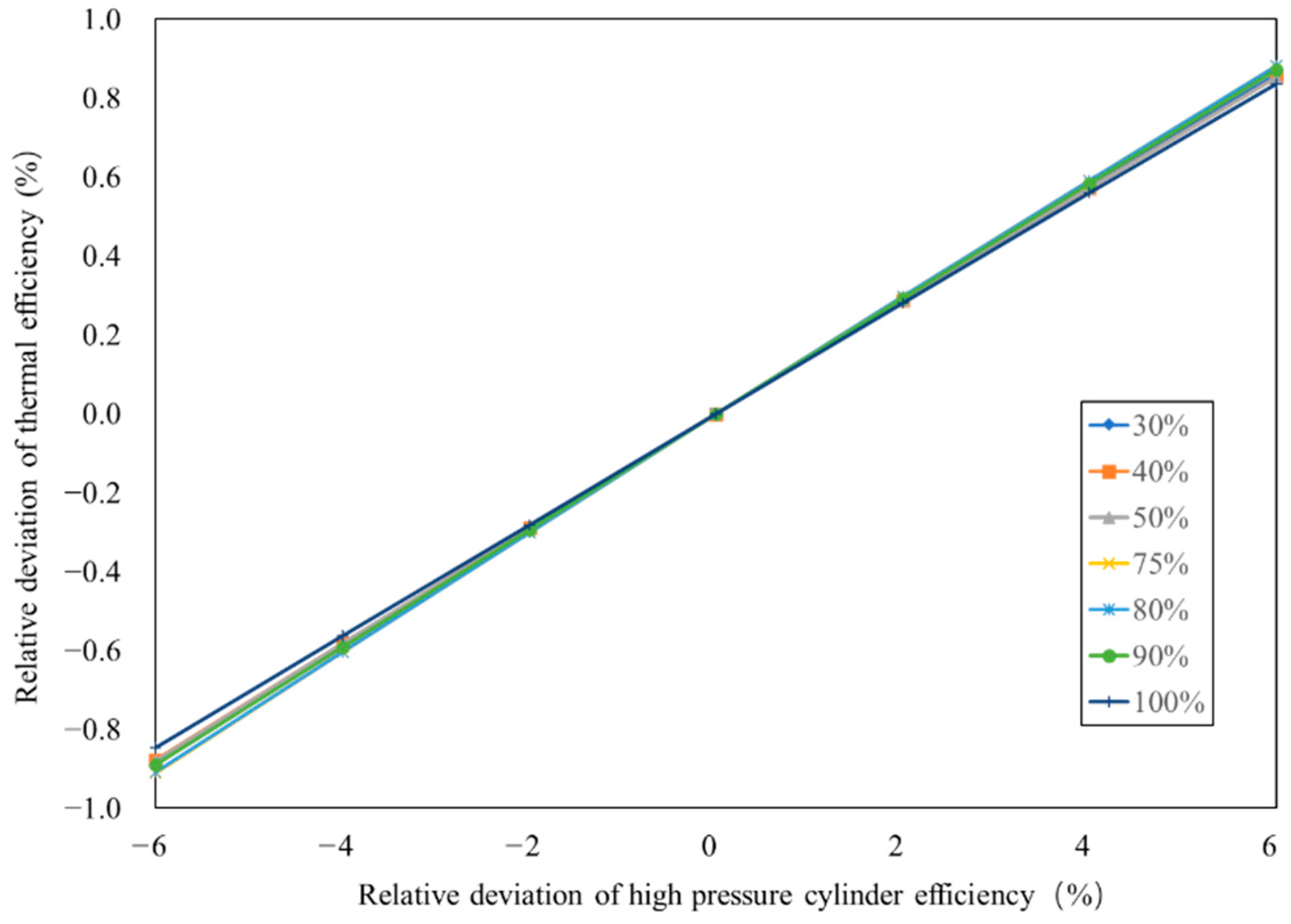
3.2.5. High-Pressure Cylinder Efficiency Disturbances

With regard to the efficiency of each cylinder of a steam turbine, the change in efficiency of medium- and low-pressure cylinders is small and has little impact on unit thermal efficiency. This is because the reheat temperature is essentially fixed during operation, so the working medium parameters at the inlet of medium- and low-pressure cylinders change little under various load conditions, and the change in efficiency is also small. The high-pressure cylinder changes greatly with load and initial parameters, which has a considerable impact on unit thermal efficiency. Therefore, the efficiency of a high-pressure cylinder is selected for study. The disturbance range is −6% to 6%, and the interval is 2%.

Figure 8 shows the variation in the relative deviation of thermal efficiency with a disturbance in the high-pressure cylinder efficiency under different output power loads. For a unit at its rated load, the unit thermal efficiency increases with the increase in high-pressure cylinder efficiency: if the high-pressure cylinder efficiency increases by 6%, then the unit thermal efficiency increases by 0.836%, or if the high-pressure cylinder efficiency decreases by 6%, then the unit thermal efficiency decreases by 0.846%.

For a unit participating in deep peak shaving, the change tendency is almost the same for different output power loads. When the unit is at 30% load, if the high-pressure cylinder efficiency increases by 6%, then the unit thermal efficiency increases by 0.86%, or if the high-pressure cylinder efficiency decreases by 6%, then the unit thermal efficiency decreases by 0.889%.

4. Conclusions

For a unit participating in deep peak shaving, a performance prediction model for the whole thermal system of a thermal power unit, including the steam turbine, heater and condenser, is established. Under operation parameter disturbance, the iterative method is adopted to realize the output of the overall state parameters and performance indexes. The following conclusions can be obtained:

(1)

The proposed prediction model is verified, with 90%, 80% and 60% load conditions selected for calculation and verification. The relative error of the unit thermal efficiency, calculated according to the prediction model, is within ±0.2%. The calculation results show that the prediction model can be verified by the actual unit test data, with high accuracy;

(2)

The rated load of the unit is 300 MW (100% load) for a unit participating in deep peak shaving, and the 90%, 80%, 75%, 50%, 40% and 30% load conditions are selected for calculation; the minimum load of the unit is 90 MW (30% load). Under each determined output power load, with an increase in the main steam temperature, reheater temperature, and high-pressure cylinder efficiency, the unit thermal efficiency increases accordingly. The unit thermal efficiency shows a downward trend with the increase in the heater end difference;

(3)

For a unit participating in deep peak shaving, when the main steam pressure in-creases compared with the reference working condition, the unit thermal efficiency decreases with the decrease in unit load; when the main steam pressure decreases compared with the reference working condition, the unit thermal efficiency increases with the decrease in unit load;

(4)

For a unit participating in deep peak shaving, the #7 heater terminal temperature difference has a greater impact on the unit thermal efficiency than the #1 heater terminal temperature difference.

References

1. Wang, J.J.; Zhang, S.; Huo, J. Dispatch optimization of thermal power unit flexibility transformation under the deep peak shaving demand based on invasive weed optimization. J. Clean. Prod. 2021, 5, 128047. [Google Scholar] [CrossRef]
2. Wu, X.; Xi, H.; Ren, Y.; Lee, K.Y. Power-Carbon Coordinated Control of BFG-Fired CCGT Power Plant Integrated with Solvent-based Post-Combustion CO2 Capture. Energy 2021, 226, 120435. [Google Scholar] [CrossRef]
3. Jiang, L.; Wang, C.; Huang, Y.; Pei, Z.; Xin, S.; Wang, W.; Brown, T. Growth in wind and sun integrating variable generation in China. IEEE Power Energy Manag. 2015, 13, 40–49. [Google Scholar] [CrossRef]
4. Chen, X.; Wu, X.; Lee, K.Y. The mutual benefits of renewables and carbon capture: Achieved by an artificial intelligent scheduling strategy. Energy Convers. Manag. 2021, 233, 113856. [Google Scholar] [CrossRef]
5. Wu, X.; Wang, M.; Liao, P.; Shen, J.; Li, Y. Solvent-based post-combustion CO2 capture for power plants: A critical review and perspective on dynamic modelling, system identification, process control and flexible operation. Appl. Energy 2020, 257, 113941. [Google Scholar] [CrossRef]
6. Mingaleeva, G.; Afanaseva, O.; Nguen, D.T.; Pham, D.N.; Zunino, P. The Integration of Hybrid Mini Thermal Power Plants into the Energy Complex of the Republic of Vietnam. Energies 2020, 13, 5848. [Google Scholar] [CrossRef]
7. Kubik, M.L.; Coker, P.J.; Barlow, J.F. Increasing thermal plant flexibility in a hig renewables power system. Appl. Energy 2015, 154, 102–111. [Google Scholar] [CrossRef] [Green Version]
8. Frew, B.A. Flexibility mechanisms and pathways to a highly renewable US electricity future. Energy 2016, 101, 65–78. [Google Scholar] [CrossRef] [Green Version]
9. Wu, X.; Shen, J.; Li, Y.; Wang, M.; Lawal, A. Flexible operation of post-combustion solvent-based carbon capture for coal-fired power plants using multi-model predictive control: A simulation study. Fuel 2018, 220, 931–941. [Google Scholar] [CrossRef] [Green Version]
10. Kwon, P.S.; Ostergaard, P. Assessment and evaluation of flexible demand in a Danish future energy scenario. Appl. Energy 2014, 134, 309–320. [Google Scholar] [CrossRef]
11. Kopiske, J.; Spieker, S.; Tsatsaronis, G. Value of power plant flexibility in power systems with high shares of variable renewables: A scenario outlook for Germany 2035. Energy 2017, 137, 823–833. [Google Scholar] [CrossRef]
12. Ye, X.; Wang, C.; Li, Q.; Shi, Z.; Liu, X.; Liu, Y. Research on optimal operation strategy with ancillary services of flexible thermal power units. In Proceedings of the 2018 Chinese Automation Congress, Xi’an, China, 30 November–2 December 2018; pp. 2990–2995. [Google Scholar]
13. Cruz, M.R.; Fitiwi, D.Z.; Santos, S.F.; Catalão, J.P. A comprehensive survey of flexibility options for supporting the low-carbon energy future. Renew. Sustain. Energy Rev. 2018, 97, 338–353. [Google Scholar] [CrossRef]
14. Eser, P.; Singh, A.; Chokani, N.; Abhari, R.S. Effect of increased renewables generation on operation of thermal power plants. Appl. Energy 2016, 164, 723–732. [Google Scholar] [CrossRef]
15. Batalla-Bejerano, J.; Trujillo-Baute, E. Impacts of intermittent renewable generation on electricity system costs. Energy Pol. 2016, 94, 411–420. [Google Scholar] [CrossRef] [Green Version]
16. Brouwer, A.S.; Van Den Broek, M.; Seebregts, A. Impacts of large-scale Intermittent Renewable Energy Sources on electricity systems, and how these can be modeled. Renew. Sustain. Energy Rev. 2014, 33, 443–466. [Google Scholar] [CrossRef]
17. Ye, L.C.; Lin, H.X.; Tukker, A. Future scenarios of variable renewable energies and flexibility requirements for thermal power plants in China. Energy 2019, 167, 708–714. [Google Scholar] [CrossRef]
18. Rodriguez, R.A.; Becker, S.; Andresen, G.B.; Heide, D.; Greiner, M. Transmission needs across a fully renewable European power system. Renew. Energy 2014, 63, 467–476. [Google Scholar] [CrossRef] [Green Version]
19. Çetin, B. Comparative energy and exergy analysis of a power plant with super-critical and sub-critical. J. Therm. Eng. 2018, 4, 2423–2431. [Google Scholar] [CrossRef]
20. Clay, J.; Mathias, J. Energetic and exergetic analysis of a multi-stage turbine, coal-fired 173 MW power plant. Int. J. Exergy 2018, 27, 419–436. [Google Scholar] [CrossRef]
21. Kumar, S.; Kumar, D.; Memon, R.A.; Wassan, M.A.; Ali, M.S. Energy and exergy analysis of a coal fired power plant. Mehran Univ. Res. J. Eng. Technol. 2018, 37, 611–624. [Google Scholar] [CrossRef]
22. Oyedepo, S.O.; Fakeye, B.A.; Mabinuori, B.; Babalola, P.O.; Leramo, R.O.; Kilanko, O.; Oyebanji, J.A. Thermodynamics analysis and performance optimization of a reheat–regenerative steam turbine power plant with feed water heaters. Fuel 2020, 280, 118577. [Google Scholar] [CrossRef]
23. Wang, Z.; Liu, M.; Zhao, Y.; Wang, C.; Chong, D.; Yan, J. Flexibility and efficiency enhancement for double-reheat coal-fired power plants by control optimization considering boiler heat storage. Energy 2020, 201, 117594. [Google Scholar] [CrossRef]
24. Zhou, J.; Ling, P.; Su, S.; Xu, J.; Xu, K.; Wang, Y.; Xiang, J. Exergy analysis of a 1000 MW single reheat advanced supercritical carbon dioxide coal-fired partial flow power plant. Fuel 2019, 255, 115777. [Google Scholar] [CrossRef]
25. Zhao, H.; Li, B.; Wang, X.; Lu, H.; Li, H. Evaluating the performance of China’s coal-fired power plants considering the coal depletion cost: A system dynamic analysis. J. Clean. Prod. 2020, 275, 122809. [Google Scholar] [CrossRef]
26. Naserabad, S.N.; Mehrpanahi, A.; Ahmadi, G. Multi-objective optimization of feed-water heater arrangement options in a steam power plant repowering. J. Clean. Prod. 2019, 220, 253–270. [Google Scholar] [CrossRef]
27. Mohammed, M.K.; Al Doori, W.H.; Jassim, A.H.; Ibrahim, T.K.; Al-Sammarraie, A.T. Energy and Exergy Analysis of the Steam Power Plant Based on Effect the Numbers of Feed Water Heater. J. Adv. Res. Fluid Mech. Therm. Sci. 2019, 56, 12. [Google Scholar]
28. De Meulenaere, R.; Maertens, T.; Sikkema, A.; Brusletto, R.; Barth, T.; Blondeau, J. Energetic and Exergetic Performances of a Retrofifitted, Large-Scale, Biomass-Fired CHP Coupled to a Steam-Explosion Biomass Upgrading Plant, a Biorefifinery Process and a High-Temperature Heat Network. Energies 2021, 14, 7720. [Google Scholar] [CrossRef]
29. Wu, T.; Wei, H.; Ge, Z.; Yang, L.; Du, X. Cooling water mass flow optimization for indirect dry cooling system of thermal power unit under variable output load. Int. J. Heat Mass Transf. 2019, 133, 1–10. [Google Scholar] [CrossRef]
30. Shen, S. Turbine Theory; China Electric Publisher: Beijing, China, 1998. [Google Scholar]
31. Elhelw, M.; Al Dahma, K.S.; Attia, A.E.H. Utilizing exergy analysis in studying the performance of steam power plant at two different operation mode. Appl. Therm. Eng. 2019, 150, 285–293. [Google Scholar] [CrossRef]
32. Zhao, Z.; Su, S.; Si, N.; Hu, S.; Wang, Y.; Xu, J.; Jiang, L.; Chen, G.; Xiang, J. Exergy analysis of the turbine system in a 1000 MW double reheat ultra-supercritical powerplant. Energy 2017, 119, 540–548. [Google Scholar] [CrossRef] [Green Version]
33. McBean, I. Steam turbine retrofifitting for power increase and effificiency enhancement. In Advances in Steam Turbines for Modern Power Plants; Woodhead Publishing: Sawston, UK, 2017. [Google Scholar]
34. Kotas, T.J. The Exergy Method of Thermal Plant Analysis; Krieger Publishing Company: Malabar, FL, USA, 1995. [Google Scholar]
35. Wei, H.; Wu, T.; Ge, Z.; Yang, L.; Du, X. Entransy analysis optimization of cooling water flow distribution in a dry cooling tower of power plant under summer crosswind. Energy 2019, 166, 1229–1240. [Google Scholar] [CrossRef]
36. Wang, W.; Zhang, H.; Liu, P.; Li, Z.; Lv, J.; Ni, W. The cooling performance of a natural draft dry cooling tower under crosswind and an enclosure approach to cooling efficiency enhancement. Appl. Energy 2017, 186, 336–346. [Google Scholar] [CrossRef]
37. Liu, S.; Shen, J.; Wang, P.H. Multi-parameter joint optimization based on steam turbine thermal system characteristic reconstruction model. In Proceedings of the IOP Conference Series: Earth and Environmental Science, Macao, China, 21–24 July 2019. [Google Scholar]
38. Wang, W.; Zhang, H.; Li, Z.; Lv, J.; Ni, W.; Li, Y. Adoption of enclosure and windbreaks to prevent the degradation of the cooling performance for a natural draft dry cooling tower under crosswind conditions. Energy 2016, 116, 1360–1369. [Google Scholar] [CrossRef]
Figure 1. Logical flowchart of the performance prediction model.
Energies 15 03171 g001
Figure 2. N300-16.5/550/550-unit thermal system.
Energies 15 03171 g002
Figure 3. Variation in the relative deviation of thermal efficiency with main steam pressure disturbance under different output power loads.
Energies 15 03171 g003
Figure 4. Variation in the relative deviation of thermal efficiency with main steam temperature disturbance under different output power loads.
Energies 15 03171 g004
Figure 5. Variation in the relative deviation of thermal efficiency with reheated steam temperature disturbance under different output power loads.
Energies 15 03171 g005
Figure 6. Variation in the relative deviation of thermal efficiency with #1 heater terminal temperature difference disturbance under different output power loads.
Energies 15 03171 g006
Figure 7. Variation in the relative deviation of thermal efficiency with #7 heater terminal temperature difference disturbance under different output power loads.
Energies 15 03171 g007
Figure 8. Variation in the relative deviation of thermal efficiency with high-pressure cylinder efficiency disturbance under different output power loads.
Energies 15 03171 g008