Steady State Modeling and Performance Analysis of a Wind Turbine-Based Doubly Fed Induction Generator System with Rotor Control

Abstract

The utilization of renewable energy sources aids in the economic development of a country. Among the various renewable energy sources, wind energy is more effective for electricity production. The doubly fed induction generator is an extensively known wind turbine generator for its partially rated power converters and dynamic performance. The doubly fed induction generator assists the wind turbine to function with a wide speed range. Hence, the steady-state performance analysis of a doubly fed induction generator helps enable it to operate efficiently at a specific wind turbine speed. In this paper, a 2 MW variable speed pitch regulated doubly fed induction generator with a speed range of 900—2000 rpm was opted for steady-state analysis. This was followed by the design and modelling of a doubly fed induction generator in Matlab/Simulink environment, and the analyses were performed using mathematical equations computed via Matlab coding. The steady-state magnitudes were calculated with rotor magnetization i_dr = 0. The closed-loop stator flux-oriented vector control is applied to the rotor side converter for controlling the designed doubly fed induction generator model. The simulation results were compared with computational values to establish a workable model with less than 10% error. The simulation model can be used for predicting the performance of the machine, fault analysis, and validation of existing DFIG at a steady state.

1. Introduction

Energy plays a vital role in the day-to-day existence of human life. A major part of energy generation comes from burning fossil fuels, such as coal and natural gas. With increasing concern over the emission of greenhouse gases and the reducing capacities of non-renewable resources, increased attention is being paid to the consumption of renewable energy sources. Renewable energy sources have a positive impact on the improvement in the economy of a country. Amid the different types of renewable energies, wind power has been extensively used for its low impact on the environment, reduced cost, and other benefits [1,2,3]. In general, the wind system tends to have fixed speed or variable speed wind turbine (WT) generators. The variable speed WT is the most popular among them for extracting the maximum energy from the wind [4]. Customary variable speed WT generators do not allow frequency regulation resulting in changes in grid frequency, and this highlights the necessity for frequency regulation technologies in WTs [4,5,6].

The doubly fed induction generator (DFIG) stands out to be one of the most sought-after systems as WT generators. In DFIG, the stator windings are directly coupled to the grid, while the rotor windings are connected through slip-rings and back-to-back voltage source converters [7]. The converter at the grid side is termed grid side converter (GSC) and at the rotor side as rotor side converter (RSC). These are coupled by DC-link, which assists to retain the voltage deviations within an acceptable range. Such a structure offers several advantages such as fixed frequency power generation under variable wind speeds, decoupled control of active and reactive power, and different operating modes. In addition, the DFIG has the choice of small converter ratings, and consequently fewer losses with better efficiency and reduced cost. At present, the DFIG structure contributes to approximately 50% of the wind power market [8]. The RSC control embraced robust stator flux-oriented vector control (FoC) as it is the most comprehensive and proven one. The purpose of the vector control is to make the AC machine behave like a DC machine, which includes carrying out a decoupling between the flux and torque components. In DFIG, the FoC allows to decouple the active and reactive powers effectively, and hence it is employed for analyzing the DFIG under a steady state (SS). Similarly, the main function of GSC control is to keep the DC-link voltage almost constant and to provide reactive power when required as per the grid codes. The control technique adopted for it is the grid voltage-oriented vector control. It also maintains the output frequency fixed on the other hand the output voltage will be adjusted in order to facilitate the active and reactive power exchange.

1.1. Literature on DFIG Steady-State Analysis (SSA)

Many attempts have been made to carry out the SSA of DFIG due to its ever-increasing popularity. However, a comprehensive SSA along with a computer simulation model and performance analysis would provide a detailed understanding of the DFIG wind turbine’s operational characteristics. With this viewpoint, the present work was carried out and the relevant literature is presented. In 2018, a SS mathematical model of DFIG was derived using the spatial vector technique under different operation zones of the wind turbine [9]. This method allows determining the operating points of any wind turbine by knowing the data and parameters of the wind turbine. In the same year, the stator flux-oriented vector control of DFIG-based wind turbines using space vector pulse width modulation was carried out and their performances were studied in [10] and found to be more effective. Later, in 2019, a computer simulation of DFIG and a vector control implementation for GSC and RSC were carried out to provide active power to the grid [11]. Subsequently, the stator field-oriented control (SFOC) of DFIM was discussed in [12], which is based on the sliding mode flux observer algorithm and the strategy is found to be effective under parameter variations. In 2020, the SSA of DFIG is presented with different magnetizing strategies for specific operating wind turbine modes [13]. This work discusses the mathematical modelling of DFIG in SS using stator flux-oriented vector control which is found too effective. In 2021, simplified SS modelling of DFIG with its operational features in a stand-alone wind energy conversion system with rotor control is discussed in [14]. Later, an SS solution to synchronous DFIG (sDFIG) orientated by references of the rotor flux for RSC and stator voltage for GSC is suggested. The analysis is summarized, and it is concluded that the sDFIG performs well when wind speed is lower than its critical value [15]. Another recent article on DFIM rotor flux orientation vector control with machine modelling for a wide speed range application is discussed in [16]. In 2022, the computation of SS values of DFIG using an accurate method for calculation is proposed in [17]. The simulation time domain results summarize that the SS values are matching with initialization values. As stated above, a comprehensive work of SS performance analysis with a working computer simulation model could be a promising work.

1.2. Significance of the Paper

The SSA of DFIG can be implemented in a global optimization environment to design the DFIG converters associated with the wind turbine. The analytical technique is a useful tool for minimizing the non-linear optimization process, which may be time-consuming and inefficient for handling digital issues. A single solution for the rotor control variables V_r and ψ exists for each SS operating point. This helps to derive the SS characteristics from a given torque-speed array emulating a three-blade wind turbine. Proper SS conditions prevent the system from numerical instability. A computer simulation study of the DFIG generation system makes it possible to create an adequate model description. The design purpose is an interpretation of the physical nature of work processes as well as the developer systems’ competency needs. The developed computer simulation shall be used to investigate the DFIG in a wide speed range of 900 to 1800 rpm. The SSA under certain operating modes provides information about the syst-em’s behavior including stator and rotor active power, power losses, current variations, and voltage variations. The overall paper structure is as follows: initially, a literature review on the present work is briefly presented with the paper’s significance in Section 1. Section 2 describes the SS mathematical modelling, MATLAB simulation and the control of a doubly fed induction generator is presented. In Section 3, the steps for implementing and analyzing the DFIG’s SS performance are presented along with the results. In Section 4, the validation of the system design with SS plots is carried out with relevant results and a comparative analysis is presented. Finally, the findings are concluded in Section 5.

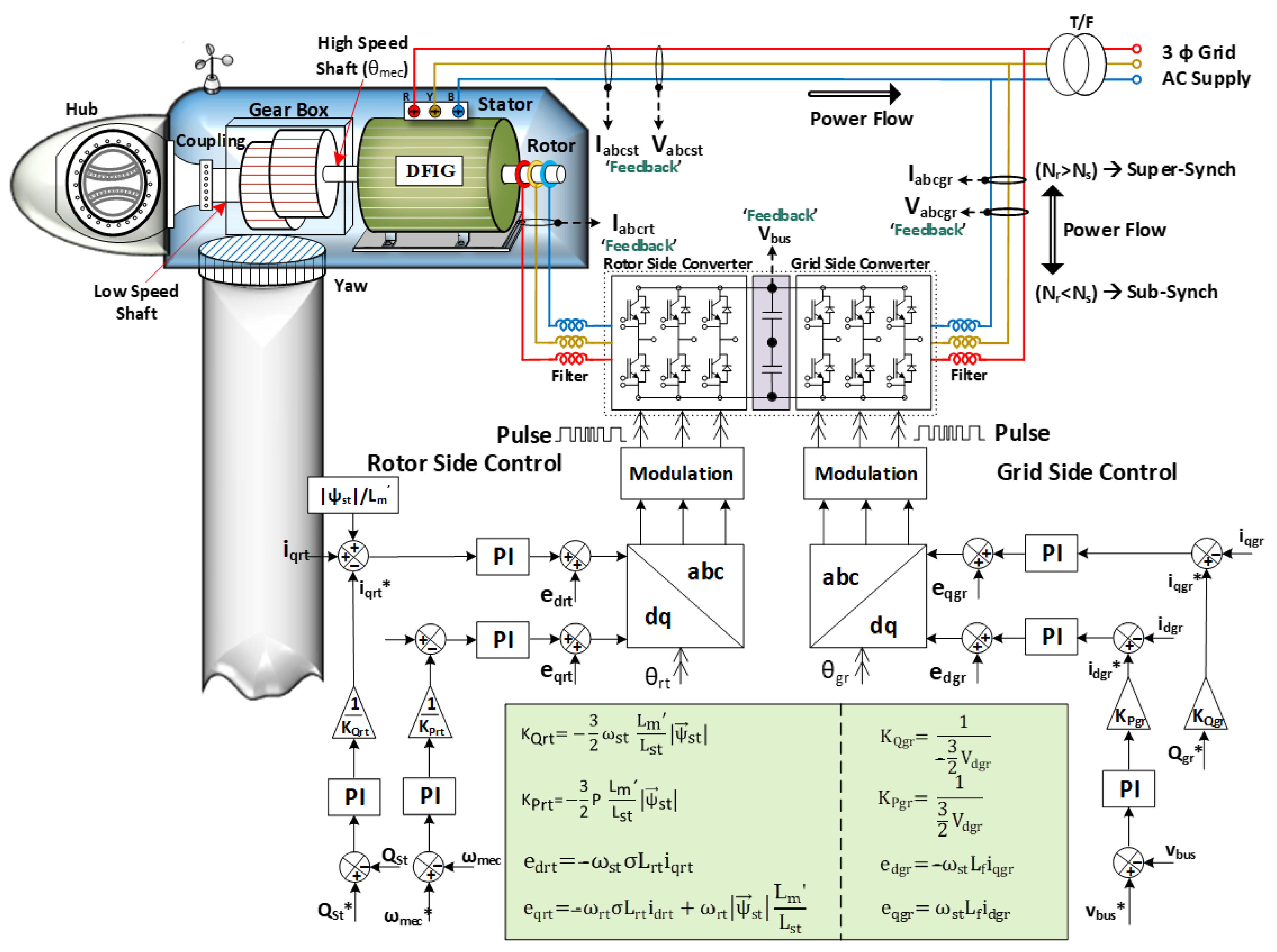
2. Modelling, Simulation, and Control of DFIG

In the wind power sector, the DFIG based wind turbine with a variable speed variable-pitch control scheme is the most prevalent wind power generator. This machine may be used as a grid-connected or stand-alone unit. To optimally extract the power from the wind and precisely predict its performance, a complete insight of the modelling, control, and SSA of this machine in both operation modes is required. In this paper, the author design and examine three-phase PWM voltage source converter models defined in the ABC and DQO synchronous reference frames, as well as their control strategies. Furthermore, utilizing Matlab/Simulink software, a DFIG-based wind turbine model coupled to a constant voltage and frequency grid is designed, as well as its associated generator control framework. This control mechanism, as well as the SS behavior of the wind plant, are clearly outlined. Figure 1 shows the DFIG models as well as the three-phase two-level PWM voltage source converter models. The control schemes are also necessary to achieve optimum output power from the wind turbine. The RSC control and the GSC control are two of these control techniques. The GSC controller is used to keep the voltage across the capacitor constant and ensure that the grid operates at a unity power factor. The torque, active power, and reactive power are all controlled by the rotor-side converter controller. As the most complete and established RSC control, it is coupled with powerful stator flux-oriented vector control. The vector control’s goal is to make the AC machine act like an independently stimulated DC machine, which involves decoupling the flux and torque components.

2.1. SS Model of DFIG

The model comprises a DFIG specifically a wound rotor induction generator which has a power converter connected to the sliprings of the rotor. The stator is directly coupled to the grid. The various parameters of the machine are defined in

Table A1. Parameters of the proposed DFIG.

Parameters	Ratings
Machine stator frequency in Hz	*fsm = 50
Machine stator power in watts	*Psm = 2 × 106
Machine rated speed in rpm	*Nm = 1500
Machine stator voltage in volts	*Vsm = 690
Machine stator current in amps	*Ism = 1760
Machine torque in Nm	*Tem = 12,732
Poles	p = 4
turns ratio (stator to rotor)	u = 1/3
Machine rotor voltage in volts	*Vrm = 2070
Slip (max)	Smax = 1/3
Machine rotor voltage referred to stator	Vrm_stator = (Vrm*smax)*u
Stator resistance in ohms	Rst = 2.6 × 10−3
Leakage inductance (stator/rotor) in Henry	Llsr = 0.087 × 10−3
Magnetizing inductance in Henry	Lm’ = 2.5 × 10−3
Rotor resistance referred to stator in ohm	Rrt = 2.9 × 10−3
Stator inductance in Henry	Lst = Lm’ + Llsr
Rotor inductance in Henry	Lrt = Lm’ + Llsr
DC bus voltage referred to stator in volts	Vbus = Vrm_stator × √2
* rated value of the machine

. For deriving the SS magnitudes of DFIG by magnetizing the machine through a rotor with i_dr = 0, the step-by-step procedure is as follows [13]. By assuming SS and the alignment of the stator flux with the d-axis, it is possible to obtain the following sets of the equation:

$${\mathrm{i}}_{\mathrm{dst}}=\frac{\left|{\overrightarrow{\mathsf{\psi }}}_{\mathrm{st}}\right|}{{\mathrm{L}}_{\mathrm{st}}}$$

(1)

$${\mathrm{i}}_{\mathrm{qst}}=-\frac{{\mathrm{L}}_{\mathrm{m}}\prime }{{\mathrm{L}}_{\mathrm{st}}}{ \mathrm{i}}_{\mathrm{qrt}}$$

(2)

$${\mathrm{v}}_{\mathrm{dst}}{=\mathrm{R}}_{\mathrm{st}}{ \mathrm{i}}_{\mathrm{dst}}$$

(3)

$${\mathrm{v}}_{\mathrm{qst}}{=\mathrm{R}}_{\mathrm{st}}{\mathrm{i}}_{\mathrm{qst}}{+\mathsf{\omega }}_{\mathrm{st}}\left|{\overrightarrow{\mathsf{\psi }}}_{\mathrm{st}}\right|$$

(4)

$${\left|\overrightarrow{{\mathrm{v}}_{\mathrm{st}}}\right|}^2{=\mathrm{v}}_{ \mathrm{dst}}^2{+\mathrm{v}}_{\mathrm{qst} }^2$$

(5)

$${\mathrm{T}}_{\mathrm{em}1}=-\frac{3}{2}\mathrm{p} \frac{{\mathrm{L}}_{\mathrm{m}}\prime }{{\mathrm{L}}_{\mathrm{st}}}\left|{\overrightarrow{\mathsf{\psi }}}_{\mathrm{st}}\right| {\mathrm{i}}_{\mathrm{qrt}}$$

(6)

First, it is necessary to calculate the stator flux amplitude of the machine. From these six sets of equations, it is easy to compute the stator flux using Equations (7)–(10). For the calculation of stator flux, we only need the parameters of the machine, stator voltages, stator currents, and torque.

$$\left|{\overrightarrow{\mathsf{\psi }}}_{\mathrm{st}}\right|=\sqrt{\frac{-\mathrm{B}\prime \pm \sqrt{\mathrm{B}\prime {}^2-4\mathrm{A}\prime \mathrm{C}\prime }}{{2\mathrm{A}}^{\prime }}}$$

(7)

$$\mathrm{A}\prime ={\left(\frac{{\mathrm{R}}_{\mathrm{st}}}{{\mathrm{L}}_{\mathrm{st}}}\right)}^2+{\mathsf{\omega }}_{\mathrm{st}}^2$$

(8)

$$\mathrm{B}\prime =\frac{4}{3} \frac{{\mathrm{R}}_{\mathrm{st}}{\mathrm{T}}_{\mathrm{em}1}{\mathsf{\omega }}_{\mathrm{st}}}{\mathrm{p}}-{\left|{\mathrm{v}}_{\mathrm{st}}\right|}^2$$

(9)

$$\mathrm{C}\prime ={\left(\frac{2}{3}\frac{{\mathrm{R}}_{\mathrm{st}}{\mathrm{T}}_{\mathrm{em}1}}{{\mathrm{pL}}_{\mathrm{m}}\prime }\right)}^2$$

(10)

Once the flux is obtained, the remaining SS magnitudes can be calculated using the below equations in a step-by-step manner. The rotor current is derived using the following three equations.

$${\mathrm{i}}_{\mathrm{drt}}=0$$

(11)

$${\mathrm{i}}_{\mathrm{qrt}}=\frac{{\mathrm{T}}_{\mathrm{em}1}}{-\frac{3}{2}\mathrm{p}\frac{{\mathrm{L}}_{\mathrm{m}}{}^{\prime }}{{\mathrm{L}}_{\mathrm{st}}} \left|{\overrightarrow{\mathsf{\psi }}}_{\mathrm{st}}\right|}$$

(12)

$${\left|\overrightarrow{{\mathrm{i}}_{\mathrm{rt}}}\right|}^2{=\mathrm{i}}_{ \mathrm{drt}}^2{+\mathrm{i}}_{\mathrm{qrt} }^2$$

(13)

The magnitude of the stator currents,

$${\left|\overrightarrow{{\mathrm{i}}_{\mathrm{st}}}\right|}^2{=\mathrm{i}}_{ \mathrm{dst}}^2{+\mathrm{i}}_{\mathrm{qst} }^2$$

(14)

The rotor speed and slip using the following two equations

$${\mathsf{\omega }}_{\mathrm{rt} }{=\mathsf{\omega }}_{\mathrm{st}} {- \mathsf{\omega }}_{\mathrm{mec}}$$

(15)

$$\mathrm{s}=\frac{{\mathsf{\omega }}_{\mathrm{rt}}}{ {\mathsf{\omega }}_{\mathrm{st}}}$$

(16)

The rotor voltages from the following three equations.

$${\mathrm{v}}_{\mathrm{drt}}{=\mathrm{R}}_{\mathrm{rt}}{\mathrm{i}}_{\mathrm{drt}}{ - \mathsf{\omega }}_{\mathrm{rt}}{\mathsf{\sigma }\mathrm{L}}_{\mathrm{rt}}{\mathrm{i}}_{\mathrm{qrt}}$$

(17)

$${\mathrm{v}}_{\mathrm{qrt}}{=\mathrm{R}}_{\mathrm{rt}}{\mathrm{i}}_{\mathrm{qrt}}{+\mathsf{\omega }}_{\mathrm{rt}}{\mathsf{\sigma }\mathrm{L}}_{\mathrm{rt}}{\mathrm{i}}_{\mathrm{qr} }{+\mathsf{\omega }}_{\mathrm{rt}}\frac{{\mathrm{L}}_{\mathrm{m}}\prime }{{\mathrm{L}}_{\mathrm{st}}}\left|{\overrightarrow{\mathsf{\psi }}}_{\mathrm{st}}\right|$$

(18)

$${\left|\overrightarrow{{\mathrm{v}}_{\mathrm{rt}}}\right|}^{2 }{=\mathrm{v}}_{ \mathrm{drt}}^2{+\mathrm{v}}_{\mathrm{qrt} }^2$$

(19)

The rotor fluxes using,

$${\mathsf{\psi }}_{\mathrm{drt}}{=\mathrm{L}}_{\mathrm{m}}{\prime \mathrm{i}}_{\mathrm{dst}}{+\mathrm{L}}_{\mathrm{rt}}{\mathrm{i}}_{\mathrm{drt}}$$

(20)

$${\mathsf{\psi }}_{\mathrm{qrt} }{=\mathrm{L}}_{\mathrm{m}}{\prime \mathrm{i}}_{\mathrm{qst} }{+\mathrm{L}}_{\mathrm{rt}}{\mathrm{i}}_{\mathrm{qrt}}$$

(21)

$${\left|\overrightarrow{{\mathsf{\psi }}_{\mathrm{rt}}}\right|}^2{=\mathsf{\psi }}_{ \mathrm{drt}}^2{+\mathsf{\psi }}_{\mathrm{qrt} }^2$$

(22)

The active powers of the machine, stator, and rotor by

$${\mathrm{P}}_{\mathrm{mec}}{=\mathrm{T}}_{\mathrm{em}1}\frac{{\mathsf{\omega }}_{\mathrm{mec}}}{\mathrm{p}}$$

(23)

$${\mathrm{P}}_{\mathrm{st}}=\frac{3}{2}{(\mathrm{v}}_{\mathrm{dst}}{\mathrm{i}}_{\mathrm{dst}}{+\mathrm{v}}_{\mathrm{qst}}{\mathrm{i}}_{\mathrm{dst}})$$

(24)

$${\mathrm{P}}_{\mathrm{rt}}=\frac{3}{2}\left({\mathrm{v}}_{\mathrm{drt}}{\mathrm{i}}_{\mathrm{drt}}{+\mathrm{v}}_{\mathrm{qrt}}{\mathrm{i}}_{\mathrm{drt}}\right)$$

(25)

The reactive powers of the stator and rotor

$${\mathrm{Q}}_{\mathrm{st}}=\frac{3}{2}{(\mathrm{v}}_{\mathrm{qst}}{\mathrm{i}}_{\mathrm{dst} }{+\mathrm{v}}_{\mathrm{dst}}{\mathrm{i}}_{\mathrm{qst}})$$

(26)

$${\mathrm{Q}}_{\mathrm{rt}}=\frac{3}{2}{(\mathrm{v}}_{\mathrm{qrt}}{\mathrm{i}}_{\mathrm{drt} }{+\mathrm{v}}_{\mathrm{drt}}{\mathrm{i}}_{\mathrm{qrt}})$$

(27)

The efficiency for motoring mode using Equation (28) and generator mode using Equation (29).

$$\left.{\mathsf{\eta }}_{\mathrm{DFIM}}=\frac{{\mathrm{P}}_{\mathrm{mec}}}{{\mathrm{P}}_{\mathrm{st}}{+\mathrm{P}}_{\mathrm{rt}}} \right|If, P_{\mathit{mec}}> 0$$

(28)

$$\left.{\mathsf{\eta }}_{\mathrm{DFIM}}=\frac{{\mathrm{P}}_{\mathrm{st}}{+\mathrm{P}}_{\mathrm{rt}}}{{ \mathrm{P}}_{\mathrm{mec}}} \right|If, P_{\mathit{mec}}< 0$$

(29)

where, i_dst, i_qst, v_dst, v_qst, i_drt, i_qrt, v_drt, v_qrt, Ψ_drt, and Ψ_qrt are the current, voltages, and flux alignment in the d-axis and q-axis. $\left|{\overrightarrow{\mathsf{\psi }}}_{\mathrm{st}}\right|$,$\left|{\overrightarrow{\mathsf{\psi }}}_{\mathrm{rt}}\right|, \left|{\overrightarrow{\mathrm{v}}}_{\mathrm{st}}\right|,\left|{\overrightarrow{\mathrm{v}}}_{\mathrm{rt}}\right|, \left|{\overrightarrow{\mathrm{i}}}_{\mathrm{st}}\right|, \mathrm{and} \left|{\overrightarrow{\mathrm{i}}}_{\mathrm{rt}}\right|$ are the magnitudes of flux, current, and voltage. T_em1, ω_st, ω_rt, ω_mec, s, P_mec, P_st, P_rt, Q_st, and Q_rt is the torque, speed, slip, active, and reactive powers of the machine. ${\mathsf{\eta }}_{\mathrm{DFIM}}$ is the efficiency of the machine.${ \mathrm{L}}_{\mathrm{m}}\prime$,${ \mathrm{L}}_{\mathrm{st}}$,${ \mathrm{L}}_{\mathrm{rt}}$, R_st, and R_rt are the self, mutual inductances, resistances of the stator, and rotor windings. The subscript notation st and rt is used to indicate the stator and rotor.

2.2. Simulation of DFIG

The overall simulation model of the electrical system, which comprises the DFIG, is shown in Figure 2. An asynchronous machine was used to represent the DFIG model with its rotor parameters referred to as the stator side. The stator was connected to a three-phase programmable voltage source. The rotor was connected to a power electronic converter RSC implemented by a universal bridge with three arms and ideal switches. We used a two-level PWM generator to control the RSC. The control signal for the PWM generator (V_{abc_ref}) came from the RSC control block. Instead of a GSC, a DC voltage source was used to simplify the system. Zero-order hold was used at the input for the control block for I_r, V_s, θ, and ω_m to make the system work as close to reality as possible. All the elements presented a constant sample time 1/f_sw. The DC voltage source had the same value as bus voltage. In the RSC control block, a field-oriented control for current loops was considered for controlling the RSC. It is discussed in the next subsection.

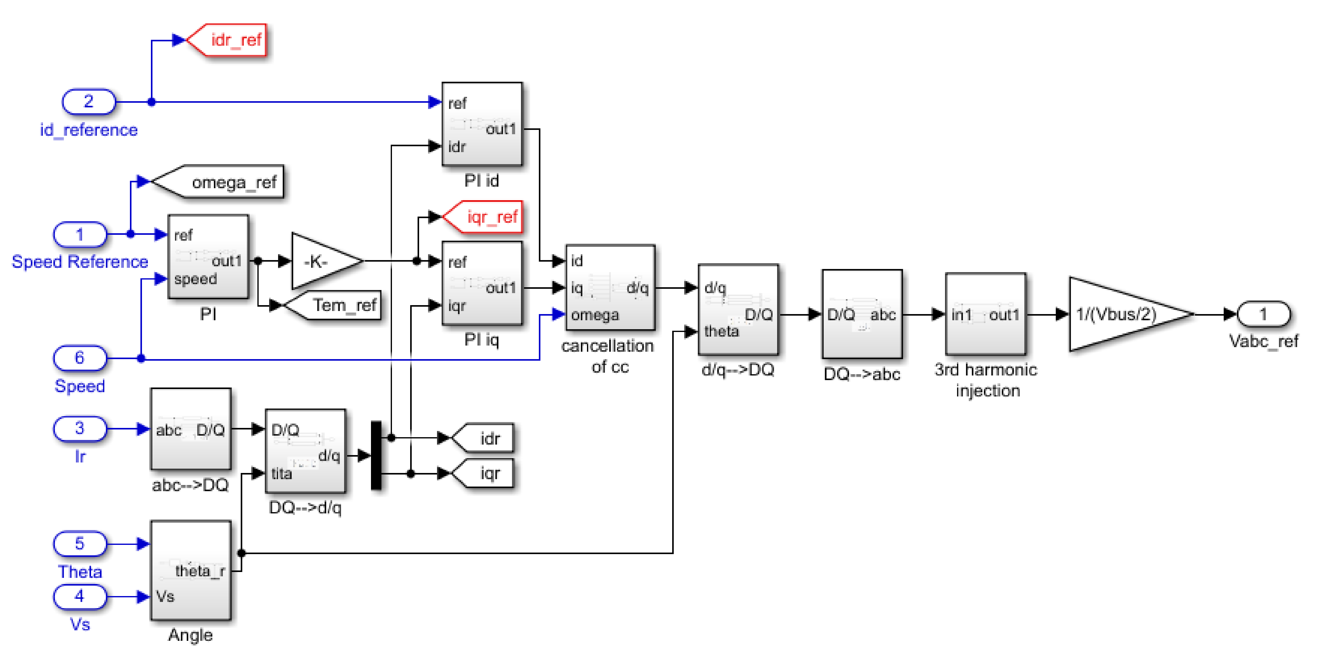
2.3. Implementation of RSC Control

The control block implemented the DFIG vector control in the synchronous reference frame as shown in Figure 3. The id reference and speed reference were initially set to zero. I_r and vs. were obtained from the three-phase measurements block and ω_m were obtained from the measurement signals output of the DFIG model.

The two inner current control loops use the transformation blocks dq to DQ, DQ to abc, abc to DQ, and DQ to dq. The PWM generator used a normalized triangular wave (−1 to 1), so the control block output was also normalized using the gain block with value 1/(V_bus/2). A third harmonic injection at the control output was used to extract more voltage for a given dc–dc bus voltage. It allowed the output voltage to be improved by 15%. The transformation angle θ_r was obtained from the stator voltages angle thetas and rotor angle θ_m. It was given as inputs to the transformation blocks. In the outer loop, a speed PI regulator was implemented to control the speed of the machine. The upper and lower limits were defined by T_em. In the inner loop, two PI regulators were required to control the id and i_q currents according to the reference values. The k_p and k_i values were found using the transfer function of the designed system. The upper and lower limits were defined by V_bus/sqrt (3). The cross-coupling terms were cancelled using the cancellation of cc block. The i_dr and i_qr were obtained from the output of transformation blocks of the rotor current Ir. The output of the speed PI regulator was multiplied by the gain to give the i_{qr_ref}. Thus, the stator flux-oriented vector control was implemented.

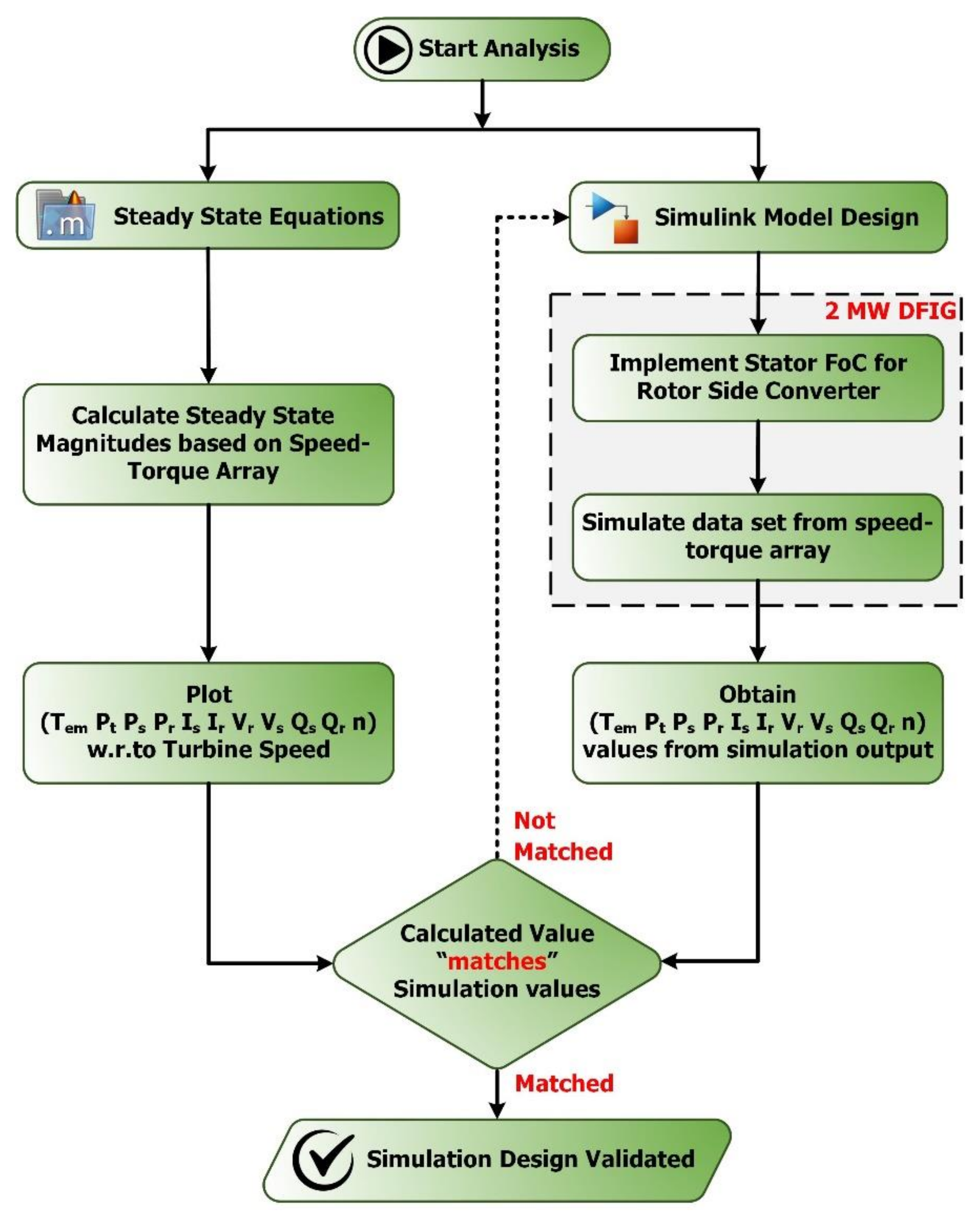
3. SS Performance Analysis of DFIG

The DFIG’s working characteristics are influenced by both the applied stator voltage and the injected rotor voltage. The direct and quadratic components of the injected rotor voltage are defined as proportional to the stator voltage for simulation purposes and are varied to observe the effect of changes in the active and reactive powers, copper losses, electromagnetic torque, power factor, and fluxes characteristics. In this article, the different operational points are used to depict DFIG’s behavior. For analyzing the performance of DFIG under SS operating conditions, the following steps are involved in the programming:

Step 1:

Start executing the program.

Step 2:

Initialize the DFIM parameters (Table A1) and read the torque-speed array for emulating a 3-blade wind turbine.

Step 3:

Check for condition, if the slip is equal to the maximum slip.

Step 4:

If true, go to step 10; Otherwise, go to step 5.

Step 5:

Calculate the stator and rotor parameters along with the mechanical parameters under each operating point extracted from the torque-speed array.

Step 6:

Determine the operating mode with mechanical torque value; go to step 7, if torque is positive; go to step 8, if torque is negative.

Step 7:

Calculate the efficiency for doubly fed induction motor; then go to step 3.

Step 8:

Calculate the efficiency for doubly fed induction generator; then go to step 3.

Step 9:

Plot the results; stator and rotor current (I_s and I_r), stator and rotor power (P_r and P_s | Q_s and Q_r), electromagnetic torque (T_em) and speed (n), and efficiency.

Step 10:

Program executed.

The SSA is mainly about the representative magnitudes of the DFIG model. The torque-speed data array as an input that emulates a 3-blade WT obtained from a 2 MW “Mitsubishi-MWT 92” wind turbine datasheet. The obtained parameters are provided in Table A1. During the execution, the SS magnitudes from a minimum speed of 900 rpm to a maximum speed of 1800 rpm are calculated. Further, through the MATLAB program, the parameters are calculated for different rotor speeds and plotted as per the Equations (1)–(29). Figure 4 shows the rotor generation strategy, that makes the d-axis rotor current zero (I_dr = 0).

Here in Figure 4a, the torque (Tem) is negative so the machine in this case operates as a generator. In Figure 4b, we have the mechanical power (Pt), which is nothing but the product of torque and speed. Then in Figure 4c, we have the active power of the rotor and stator (Pr and Ps). The maximum active power is around 2 MW. Max rotor power is around 400 kW. The active power of the rotor is negative and positive depending on the rotational speed. In Figure 4d,e, we have the stator (Is) and rotor currents (Ir). The rotor current is bigger than the stator current. Accordingly, in Figure 4g,h, we have the stator reactive power (Qs) and rotor reactive power (Qr). We can see that Qs increase with the rise in rotor speed whereas Qr decreases with a rise in rotor speed. Then, in Figure 4f we have the stator (Vs) and rotor voltages (Vr). We can see that the stator is directly connected to the grid, so the stator voltage amplitude is always constant. Whereas the rotor voltage magnitudes depend on the speed. At synchronous speed, it is minimum. At the two extremes, we have high voltages. We are working with a rotor referred to as the stator, so these magnitudes are not real magnitudes. If we convert to the rotor side and work, we will have the voltages very near to stator voltages. Finally, in Figure 4i we have the efficiency of the DFIG at a SS.

Here, we have the mechanical power (P_m), which is nothing but the product of torque and speed. Then we have the active power of the rotor and stator (P_r and P_s). The stator active power is much bigger than the rotor active power. The maximum active power is around 2 MW. Max rotor power is around 400 kW. The active power of the rotor is negative and positive depending on the rotational speed: the stator currents, red Q_r = 0 and blue for I_dr = 0. When we make Q_r = 0, the I_s is lower than when I_dr = 0. On the contrary, for the rotor current, we see that with I_dr = 0, the rotor current is lower. Then we have the stator and rotor voltages. We can see that the stator is directly connected to the grid, so the stator voltage amplitude is always constant. Whereas the rotor voltage magnitudes depend on the speed. At synchronous speed, it is minimum. At the two extremes, we have high voltages. We are working with a rotor referred to as the stator, so these magnitudes are not real magnitudes. If we convert to the rotor side and work, we will have the voltages very near to stator voltages. Then we have the reactive power. With I_dr = 0, we have high reactive power, and with the other generation strategy, which has 0 reactive power. Finally, rotor reactive power behavior in both cases, and finally, we have the efficiency.

The steps followed for the analysis using SS equations are discussed as a flowchart in Figure 5. The left branch discusses the computational method using mathematical equations. The right branch discusses the performance analysis of DFIG using the MATLAB/Simulink model. In the end, the results are compared to validate the simulation.

4. Results and Discussion

The developed model is simulated in the following procedure for obtaining the results,

Step 1:

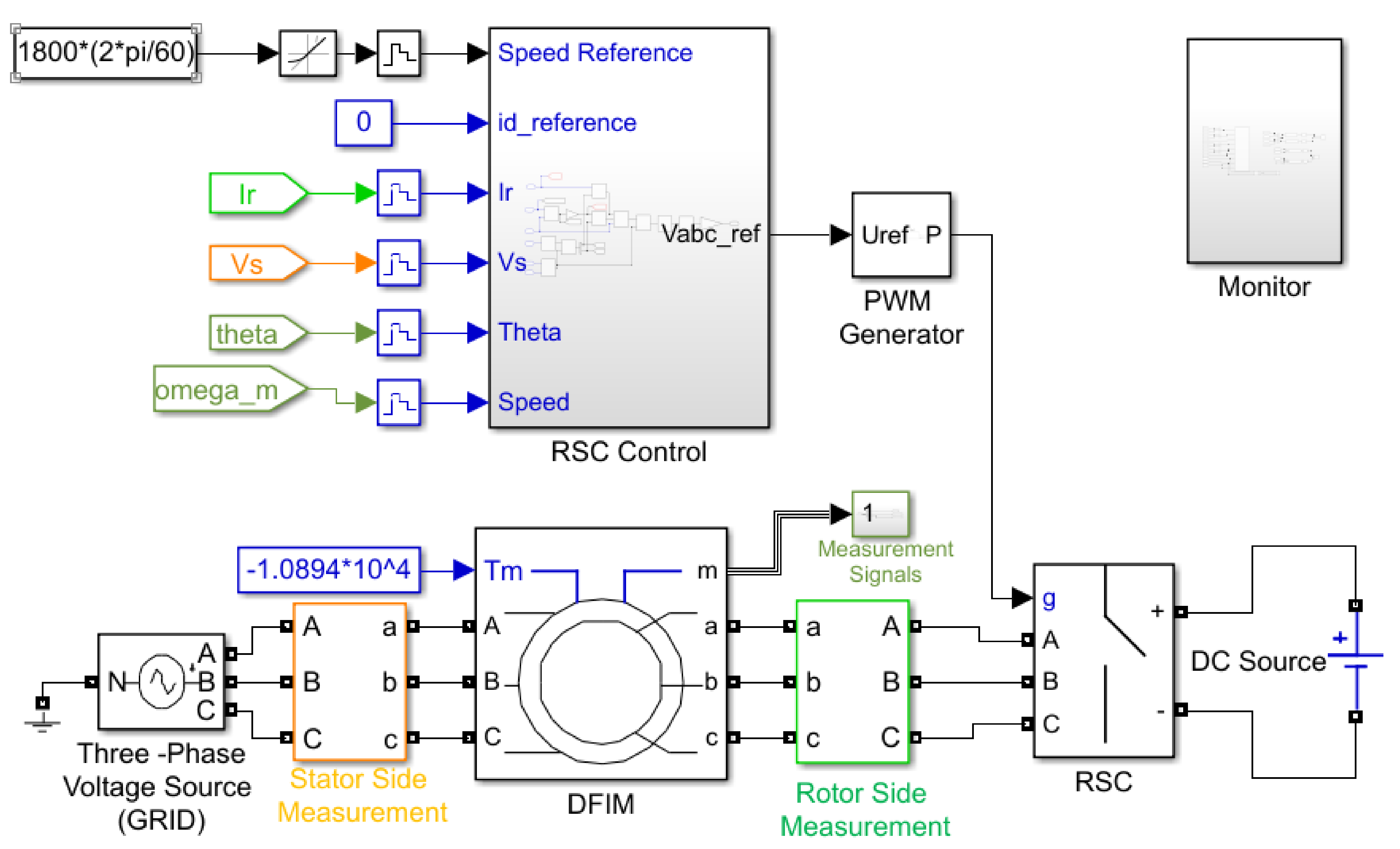
From the SS graph, the values are selected corresponding to the speed, of 1800 rpm. Thus, the speed reference is given as 1800*(2*pi/60).

Step 2:

The rate limiter for speed variation is set with the slew rate of 100 radians per second (100/1).

Step 3:

Set the load torque of simulation to −10,894 Nm corresponding to the speed of 1800 rpm. The negative torque signifies generator mode.

Step 4:

The time constant of the speed PI regulator is reduced to 1/4th of its value to make the speed regulator work four times faster.

Step 5:

Strong perturbation is caused because the machine is directly connected to the grid, which is not done in practical situations. The startup transient is ignored as the focus of this work to analyze the machine under SS.

Step 6:

Run the simulation.

4.1. Simulation Results

The simulation results of SSA at two different operating points of 1800 rpm with load torque of −10,894 and 1273.21 rpm with a torque of −5285, can be seen in Figure 6a,b. The change in operating point is initiated at a time instant of 6 s through a step signal. For a smooth transition, a rate limiter has been used with a rate of 100/seconds. The model is run with a reference speed of 1273.21 rpm and torque of −5285 Nm and at 6 s, the rotor reference speed is changed to 188.4 rad/s ((1364 rev/min × 2π rad/rev)/(60s/min) = 188.4 rad/s) corresponding to 1800 rpm. The operating point shifts from subsynchronous mode to super-synchronous mode. The synchronous speed of the machine is 1500 rpm. The new SS is reached at 6.5 s. The speed controller tracks the reference value for both subsynchronous and super-synchronous modes. The machine operates in subsynchronous mode and later switches to super-synchronous speed as per the reference. The rotor and stator currents have the value corresponding to the specific operating point in Figure 5 corresponding to a rotational speed of 1273.2 rpm and 1800 rpm with rotor magnetizing technique (idr = 0). The rotor voltages (sqrt(Vdr^2 + Vqr^2)) also follow the same. The absolute active power and reactive powers of the system will be obtained with correct voltages and currents.

The I_dref (Figure 5e) is maintained at 0, as we maintain reactive power at zero during a SS. The I_q current (Figure 5d) varies from 1176 A to 2103 A, to reach the new operating point corresponding to a speed-torque (1800 rpm & −10,602 Nm). I_q is responsible for controlling the torque. The current controllers work properly as the d and q component currents follow the reference. The rotor voltages V_d and V_q (Figure 5g,h) vary in such a way that along with the rotor current, the generator generates the required real power of approximately 130 kw and 323 kw. The stator voltage in Figure 5c is constant with a peak amplitude of 563 V as no variation is made at the stator. The stator current in Figure 5f changes from 1362 A to 2079 A as the stator of the generator nearing synchronous speed draws less power. The rotor current in Figure 5i changes from 1174.5 A corresponding to a SS of 133 rad/sec and during synchronous speed, the frequency of rotor current becomes zero (DC). After crossing synchronous speed, the generator operates at super synchronous speed with a rotor current of 2019 peak amplitude. The machine operates as a conventional 3 phase synchronous generator.

4.2. Comparative Analysis

The steps followed for the analysis using SS equations are discussed in the flowchart, depicted in Figure 6. The left branch discusses the computational method using mathematical equations. The right branch discusses the performance analysis of DFIG using the MATLAB/Simulink model. In the end, the results are compared to validate the simulation.

Figure 6. Process of DFIG’s SS performance analysis.

Figure 6. Process of DFIG’s SS performance analysis.

The most representative SS magnitudes of DFIG and they are compared to the calculated SS values available in Figure 5 corresponding to Idr = 0 for a rotational speed of 1800 rpm and 1273.21 rpm. It is observed that the SS magnitudes both computed and simulated are similar in Figure 7, Figure 8, Figure 9, Figure 10, Figure 11, Figure 12, Figure 13 and Figure 14. The results are tabulated for further analysis. The SS magnitudes obtained through programming for two different operating points corresponding to a speed of 1800 rpm and 1273.21 rpm are shown in Figure 7a, Figure 8a, Figure 9a, Figure 10a, Figure 11a, Figure 12a, Figure 13a and Figure 14a. The simulation model is run for these two operating points from 0 s to 6 s for a speed of 1273.21 rpm and from 6 s to 10 s for a speed of 1800 rpm. The most significant magnitudes are shown in Figure 7b, Figure 8b, Figure 9b, Figure 10b, Figure 11b, Figure 12b, Figure 13b and Figure 14b. The values of stator current are calculated to be 1200.52 A, which is similar to the simulated SS value of 1362.82 A for a speed of 1273.21 rpm. Again, for a speed of 1800 rpm, the calculated value of stator current is 2124.85 A and the SS value of 2079.7 A is within comparable limits. Figure 7a,b show the values for comparison.

Figure 7. (a) Calculated stator current; (b) Stator current of the designed system.

Figure 7. (a) Calculated stator current; (b) Stator current of the designed system.

The values of rotor current are calculated to be 1011.98 A, which is similar to the simulated SS value of 1214.42 A for a speed of 1273.21 rpm. Again, for a speed of 1800 rpm, the calculated value of stator current is 2076.2 A and the SS value of 2114.37 A is within comparable limits. Figure 8a,b show the values for comparison.

Figure 8. (a) Calculated rotor current; (b) Rotor current of the designed system.

Figure 8. (a) Calculated rotor current; (b) Rotor current of the designed system.

The values of stator voltage are calculated to be 563.383 V, which is similar to the simulated SS value of 563.382 V for all operating points as the stator voltage remains constant. Figure 9a,b show the values for comparison.

Figure 9. (a) Calculated stator voltage; (b) Stator voltage of the designed system.

Figure 9. (a) Calculated stator voltage; (b) Stator voltage of the designed system.

The values of rotor voltages are calculated to be 86.0158 V, which is similar to the simulated SS value of 87.1958 V for a speed of 1273.21 rpm. Again, for a speed of 1800 rpm, the calculated value of stator current is 106.294 V and the SS value of 104.47 V is within comparable limits. Figure 10a,b show the values for comparison.

Figure 10. (a) Calculated rotor voltage; (b) Rotor voltage of the designed system.

Figure 10. (a) Calculated rotor voltage; (b) Rotor voltage of the designed system.

The stator real power in Figure 11b, varies from 824.698 kW to 1693.45 kW corresponding to a speed of 133.33 rad/sec (1273.21 rpm) to 188.5 rad/sec (1800 rpm) and is comparable with the calculated value of −824.545 kW and −1693.620 kW as shown in Figure 11a. The stator real power in Figure 12b, varies from 824.698 kW to 1693.45 kW corresponding to a speed of 133.33 rad/sec (1273.21 rpm) to 188.5 rad/sec (1800 rpm). With a transition peak of 261.395 kW. The stator reactive power in Figure 13b, remains constant at 589.357 kVAR. The rotor real power in Figure 11b varies from 130.217 kW to 319.068 kW corresponding to a speed of 133.33 rad/sec (1273.21 rpm) to 188.5 rad/sec(1800 rpm). The rotor reactive power in Figure 13b changes from 14.067 kVAR to −64.57 kVAR to meet the reactive power demands during subsynchronous and super-synchronous conditions.

Figure 11. (a) Calculated stator real power; (b) Stator real power of the designed system.

Figure 11. (a) Calculated stator real power; (b) Stator real power of the designed system.

Figure 12. (a) Calculated rotor real power; (b) Rotor real power of the designed system.

Figure 12. (a) Calculated rotor real power; (b) Rotor real power of the designed system.

The stator reactive power in Figure 13b, varies from 589.357 kVAR to 590.238 kVAR for change in speed from 1273.21 rpm to 1800 rpm. This is similar to the calculated values of 591.097 kVAR and 596.696 kVAR in Figure 13a.

Figure 13. (a) Calculated stator reactive power; (b) Stator reactive power of the designed system.

Figure 13. (a) Calculated stator reactive power; (b) Stator reactive power of the designed system.

The rotor reactive power in Figure 14b changes from 14.067 kVAR to −64.57 kVAR to meet the reactive power demands during subsynchronous and super-synchronous conditions. The values are comparable to the calculated values of 12.4827 kVAR and −69.5111 kVAR in Figure 14a.

Figure 14. (a) Calculated rotor reactive power; (b) Rotor reactive power of the designed system.

Figure 14. (a) Calculated rotor reactive power; (b) Rotor reactive power of the designed system.

The values of I_s, I_r, V_s, V_r, P_s, P_r, Q_s, and Q_r obtained through computation and simulation for the specific operating point are tabulated in

Table 1. Comparison of SS magnitudes.

SS Magnitudes	Nr = 1273.21 rpm/T = −5285 Nm			Nr = 1800 rpm/T = −10,894 Nm
	Computed Values	Simulated Values	Error (%)	Computed Values	Simulated Values	Error (%)
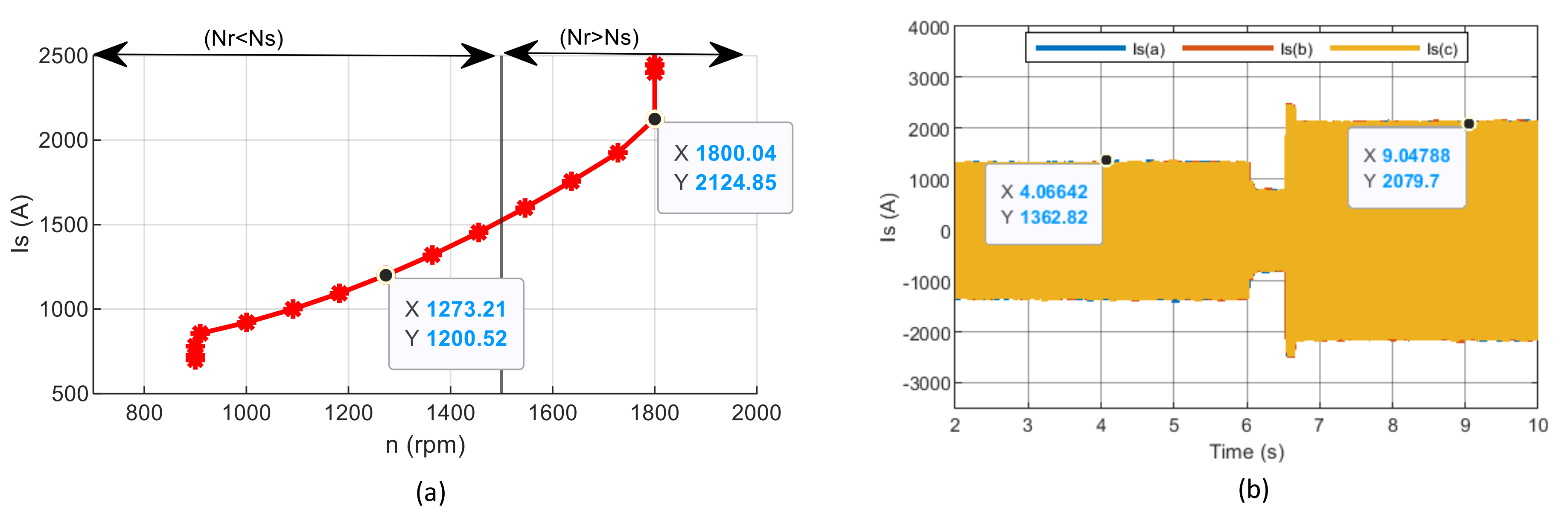
Stator Current (Is) (A)	1200.52	1362.82	13.51 ↑↑	2124.85	2079.7	2.12 ↓↓
Rotor Current (Ir) (A)	1011.98	1194.6	18.04 ↓↓	2076.2	2114.37	1.83 ↑↑
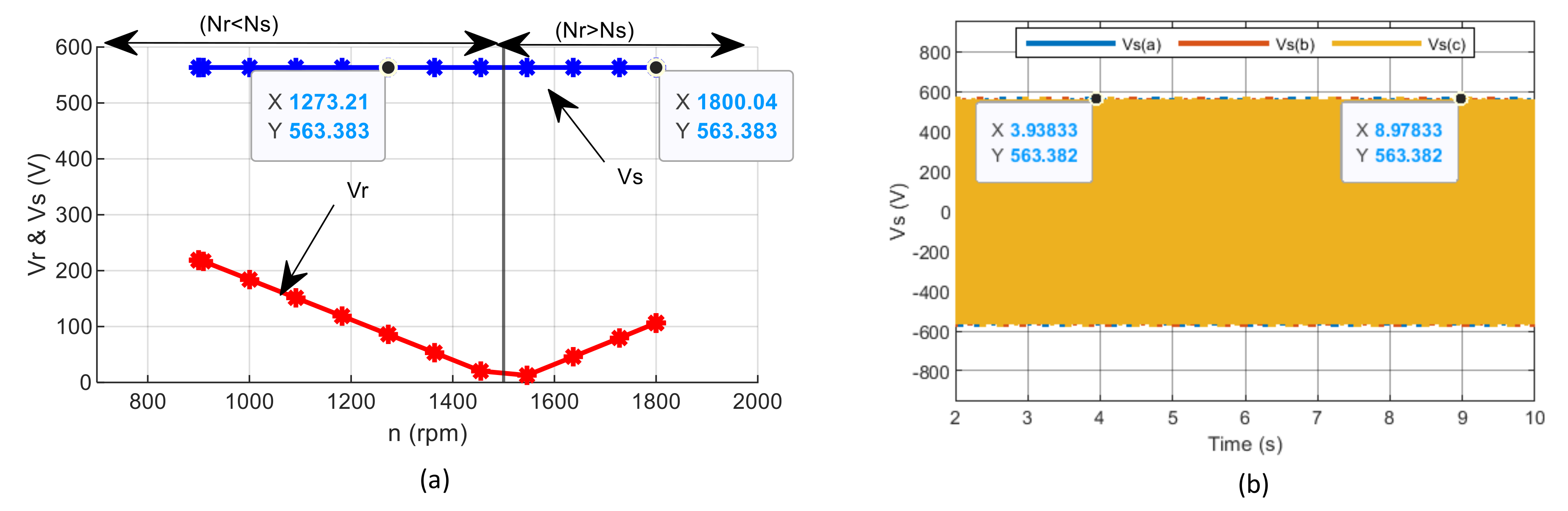
Stator Voltage (Vs) (V)	563.383	563.382	--	563.383	563.382	--
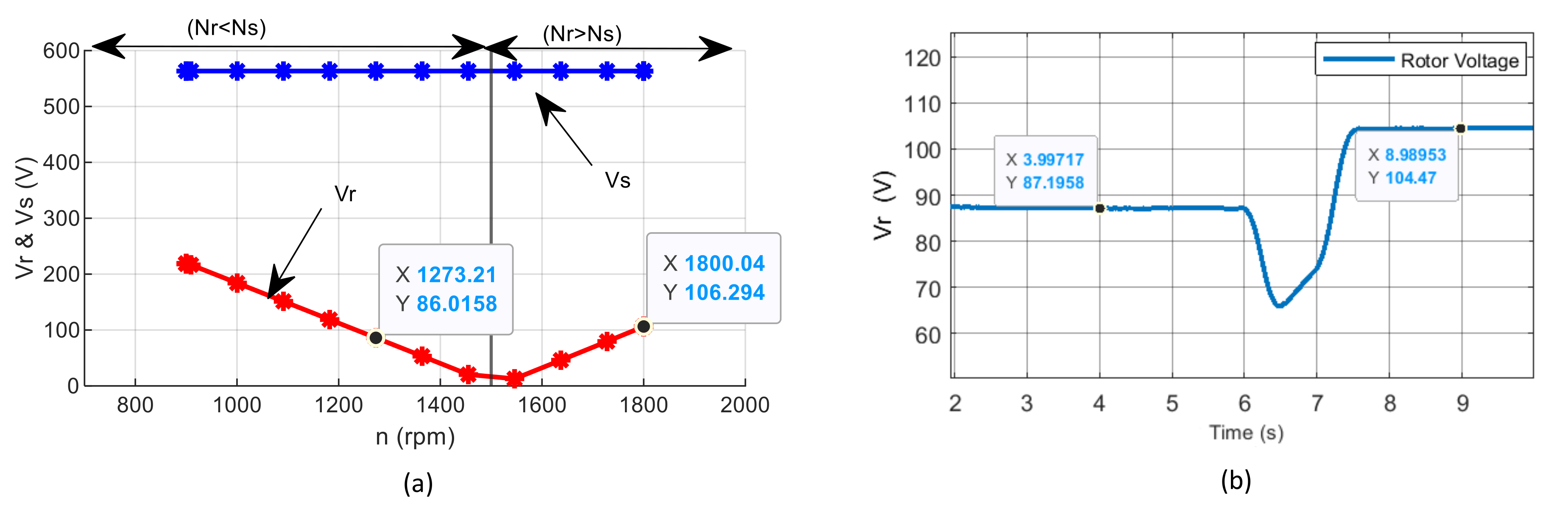
Rotor Voltage (Vr) (V)	86.0158	87.1958	1.37 ↑↑	106.294	104.47	1.71 ↓↓
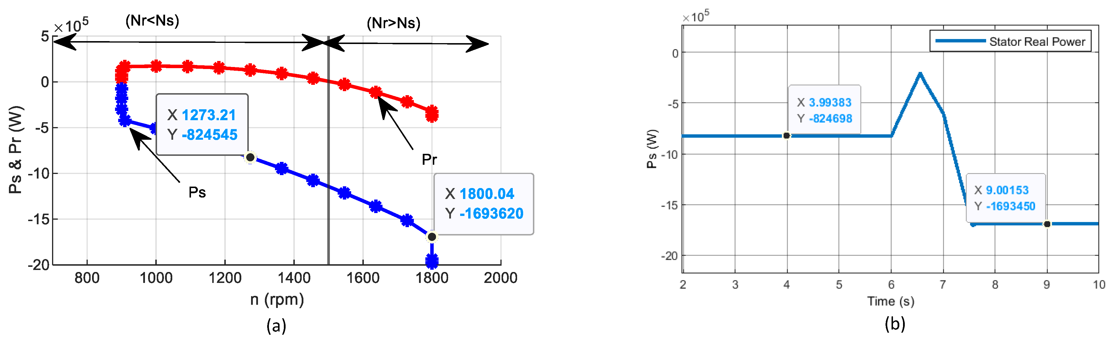
Stator Real Power (Ps) (W)	−824,545	−824,698	--	−1,693,620	−1,693,450	--
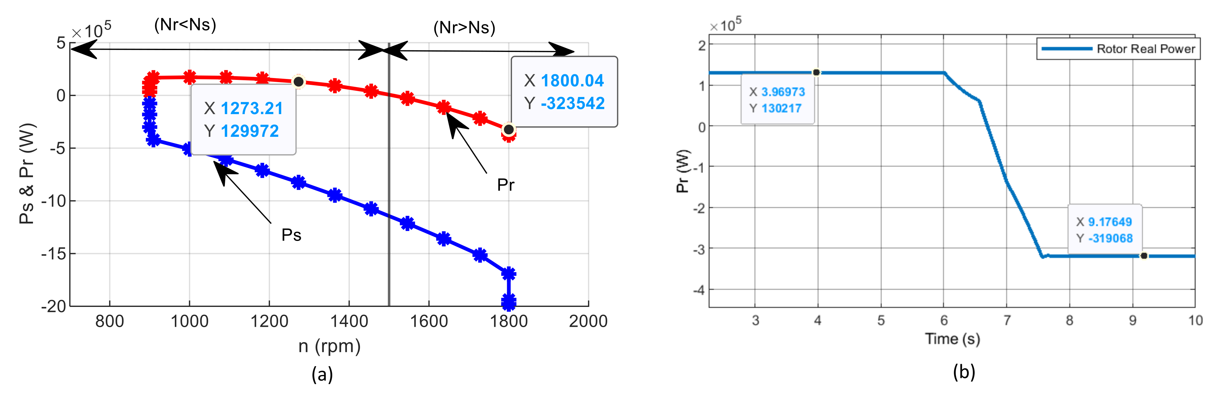
Rotor Real Power (Pr) (W)	129,972	130,217	0.18 ↑↑	−323,542	−319,068	1.38 ↓↓
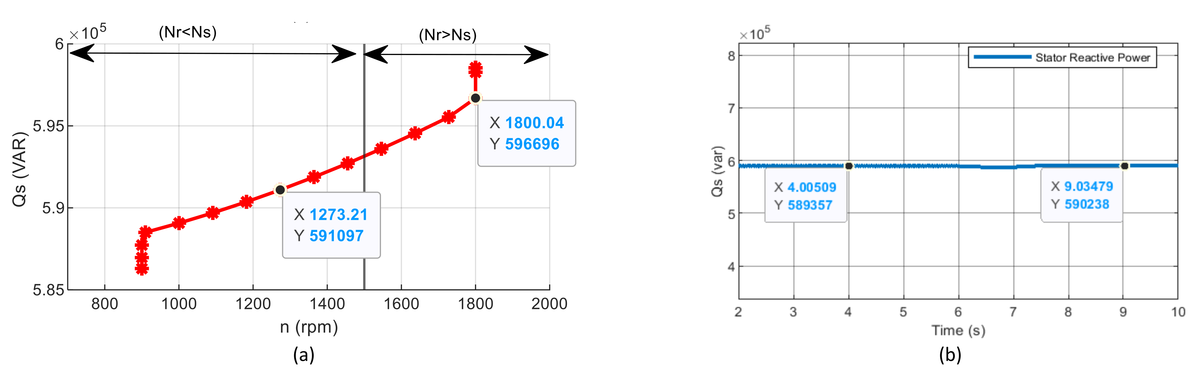
Stator Reactive Power (Qs) (VAR)	591,097	589,357	0.29 ↓↓	596,696	590,238	1.08 ↓↓
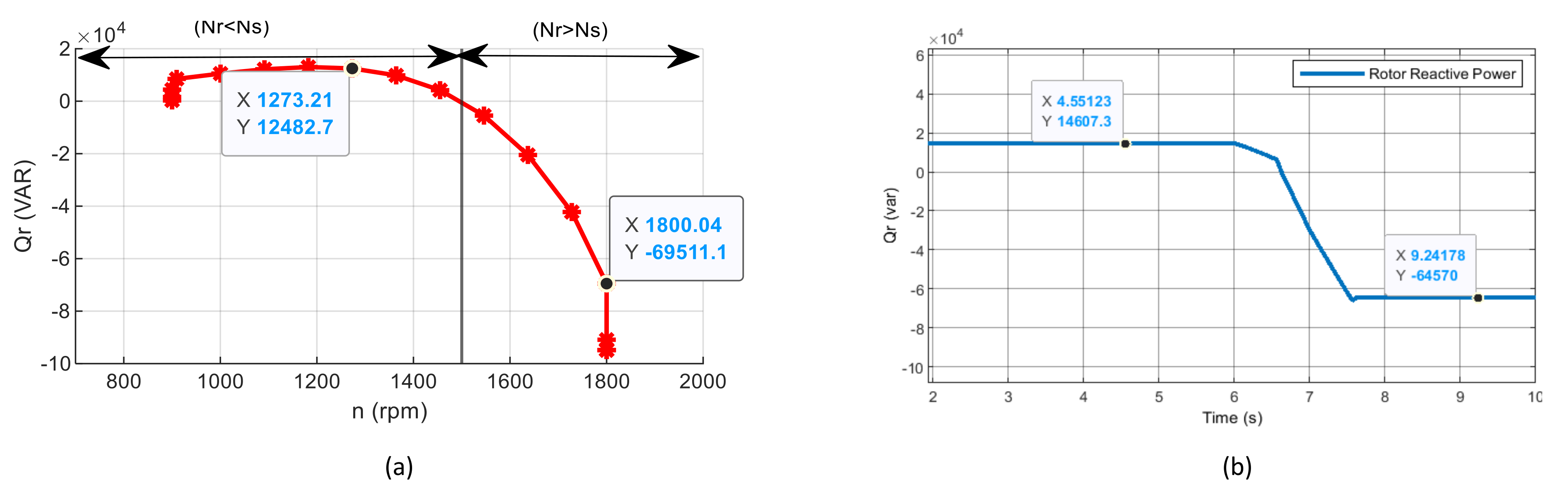
Rotor Reactive Power (Qr) (VAR)	12,482.7	14,607.3	17.02 ↑↑	−69,511.1	−64,570	7.10 ↓↓

↑↑ indicates percentage increased from computed value; ↓↓ percentage decreased from the computed value.

. The error between the computed and simulated values are calculated and it is found that an overall error of less than 10% is observed for a speed of 1800 rpm and an error of less than 20% is observed for an operating speed of 1273.21 rpm. Hence, it is established from the acquired results that the designed system is working properly and can be used for future analysis.

5. Conclusions

In this paper, the SS performance analysis of the DFIG based WT with rotor magnetizing strategy I_dr = 0 and the DFIG system design in MATLAB/Simulink is presented. For the analysis, a 2 MW DFIG WT was chosen with torque-speed datasets of an MWT 92 Mitsubishi WT design. The SS magnitudes of the DFIG were computed based on SS equations and the values were plotted. These SS values were further used for the validation of the designed system for a specific operating mode corresponding to a rotor speed of 1800 rpm. The simulation results were, in turn, compared with the calculated value and the overall error in SS magnitudes was found to be less than 10% which shows the acceptable performance of the designed system. The designed system can be used by the scientific community for a detailed study of the wind turbine based DFIG such as WT behavior under fault, performance under various test conditions, and for further research on the topic.

References

- Ntanos, S.; Skordoulis, M.; Kyriakopoulos, G.; Arabatzis, G.; Chalikias, M.; Galatsidas, S.; Batzios, A.; Katsarou, A. Renewable Energy and Economic Growth: Evidence from European Countries. Sustainability 2018, 10, 2626. [Google Scholar] [CrossRef] [Green Version]
- Sawant, M.; Thakare, S.; Rao, A.P.; Feijóo-Lorenzo, A.E.; Bokde, N.D. A Review on State-of-the-Art Reviews in Wind-Turbine- and Wind-Farm-Related Topics. Energies 2021, 14, 2041. [Google Scholar] [CrossRef]
- Javadi, M.A.; Ghomashi, H.; Taherinezhad, M.; Nazarahari, M.; Ghasemiasl, R. Comparison of Monte Carlo Simulation and Genetic Algorithm in Optimal Wind Farm Layout Design in Manjil Site Based on Jensen Model. In Proceedings of the 2021 7th Iran Wind Energy Conference (IWEC2021), Shahrood, Iran, 17–18 May 2021. [Google Scholar]
- Artigao, E.; Martín-Martínez, S.; Honrubia-Escribano, A.; Gómez-Lázaro, E. Wind turbine reliability: A comprehensive review towards effective condition monitoring development. Appl. Energy 2018, 228, 1569–1583. [Google Scholar] [CrossRef]
- Li, Q.; Cherian, J.; Shabbir, M.S.; Sial, M.S.; Li, J.; Mester, I.; Badulescu, A. Exploring the Relationship between Renewable Energy Sources and Economic Growth. The Case of SAARC Countries. Energies 2021, 14, 520. [Google Scholar] [CrossRef]
- Dao, C.; Kazemtabrizi, B.; Crabtree, C. Wind turbine reliability data review and impacts on levelised cost of energy. Wind. Energy 2019, 22, 1848–1871. [Google Scholar] [CrossRef] [Green Version]
- Justo, J.J.; Mwasilu, F.; Jung, J.W. Doubly-fed induction generator-based wind turbines: A comprehensive review of fault ride-through strategies. Renew. Sustain. Energy Rev. 2015, 45, 447–467. [Google Scholar] [CrossRef]
- Hossain, M.E. A new approach for transient stability improvement of a grid-connected doubly fed induction genera-tor–based wind generator. Wind Eng. 2017, 41, 245–259. [Google Scholar] [CrossRef]
- Quispe, M.I.C.; Cárdenas, F.V.C.; Quispe, E.C. A Method for Steady State Analysis of Doubly Fed Induction Generator. In Proceedings of the 2018 IEEE ANDESCON, Santiago de Cali, Colombia, 22–24 August 2018. [Google Scholar]
- Nora, Z.; Nadia, B.; Nadia, B.S.A. Contribution to PI Control Speed of a Doubly Fed Induction Motor. In Proceedings of the 2018 6th International Conference on Control Engineering & Information Technology (CEIT), Istanbul, Turkey, 25–27 October 2018. [Google Scholar]
- Nam, N.H. Modeling, Algorithm Control And Simulation Of Variable-Speed Doubly-Fed Induction Generator In Grid Connected Operation. In Proceedings of the 2019 26th International Workshop on Electric Drives: Improvement in Efficiency of Electric Drives (IWED), Moscow, Russia, 30 January–2 February 2019. [Google Scholar]
- Zerzeri, M.; Jallali, F.; Khedher, A. Robust FOC Analysis of a DFIM using an SMFO: Application to Electric Vehicles. In Proceedings of the 2019 International Conference on Signal, Control and Communication (SCC), Hammamet, Tunisia, 16–18 December 2019. [Google Scholar]
- Naveed, I.; Zhao, G.; Yamin, Z.; Gul, W. Steady State Performance Analysis of DFIG with Different Magnetizing Strategies in a Pitch-Regulated Variable Speed Wind Turbine. In Proceedings of the 2020 4th International Conference on Power and Energy Engineering (ICPEE), Xiamen, China, 19–21 November 2020. [Google Scholar]
- Sharawy, M.; Shaltout, A.A.; Abdel-Rahim, N.; Youssef, O.E.M.; Al-Ahmar, M.A. Simplified Steady State Analysis of Stand-Alone Doubly Fed Induction Generator. In Proceedings of the 2021 22nd International Middle East Power Systems Conference (MEPCON), Assiut, Egypt, 14–16 December 2021. [Google Scholar]
- Li, S.; Li, L. Steady-state Solution and Evaluation Indices of DFIG Operating at Synchronous Speed (sDFIG). In Proceedings of the 2021 IEEE Sustainable Power and Energy Conference (iSPEC), Nanjing, China, 23–25 December 2021. [Google Scholar]
- Arjun, G.T.; Jyothi, N.S.; Neethu, V.S. Vector Control of Doubly fed Induction Machine for an Electric Vehicle Application. In Proceedings of the 2021 International Conference on Recent Trends on Electronics, Information, Communication & Technology (RTEICT), Bangalore, India, 27–28 August 2021. [Google Scholar]
- Karthik, D.R.; Kotian, S.M.; Manjarekar, N.S. An Accurate Method for Steady State Initialization of Doubly Fed Induction Generator. In Proceedings of the 2022 IEEE International Conference on Power Electronics, Smart Grid, and Renewable Energy (PESGRE), Trivandrum, India, 2–5 January 2022. [Google Scholar]