Study on the Dynamic Ice Load of Offshore Wind Turbines with Installed Ice-Breaking Cones in Cold Regions

Abstract

The dynamic ice load of conical offshore wind turbines (OWTs) in cold regions is unclear. The ice force period is the key parameter used to establish an ice force model for conical structures. To obtain ice load data, a field monitoring system was installed on an OWT in a cold region in China. Based on the monitoring data, a new formula for calculating the ice force period of conical structures was established. By comparing the period calculated with this formula and the measured ice force period, it was found that the calculated data generally agreed with the measured data. Then, a random dynamic ice force model for conical OWTs can be established. Based on this ice force model, the ice-induced vibration of an OWT was analyzed with the ANSYS finite element software. The results are in good agreement with the measured data obtained from the OWT in the time and frequency domains. Therefore, the random dynamic ice force model established in this paper can be used to evaluate the ice resistance performance of conical OWTs in cold regions.

1. Introduction

Marine wind energy resources have greatly expanded in recent years. Excellent progress has also been made in the design, construction and installation of large and superlarge offshore wind turbine (OWT) structures. Complex marine environmental loads are the main factors that affect the structural safety of OWTs, especially for wind farms built in ice-covered sea areas. Wang et al. analyzed the influence of ice-induced vibrations (IIVs) on OWTs in the Bohai Sea through a numerical method, and found that the acceleration response at the top of the OWT was significantly caused by IIV [1]. Lou analyzed and compared the fatigue damage caused by IIVs and the fatigue damage caused by wind load on OWTs in the Bohai Sea, and found that they were equivalent [2]. Based on the Matlock model and the Määttänen model, Ye et al. simulated the IIVs on OWTs, and found that IIVs had a great impact on OWTs, especially for the tower [3]. Therefore, ice loads are one of the controlling loads for OWTs. Hendrikse et al. studied ice interactions between ice and vertical OWTs when the frequency lock-in phenomenon occurred [4]. Based on the existing theory, Seidel et al. established an evaluation method for the frequency lock-in phenomenon of OWTs [5]. At present, the ice load influences on OWTs and the ice-resistant design of OWTs have become key issues for wind farms in cold regions. When sea ice interacts with different types of structures, the breaking failure characteristics of sea ice can differ. According to the regulations of Q/HSn 3000-2002 [6], the design compression strength of sea ice in China’s sea areas is greater than the design bending strength, and most of the design compression strength is about three times greater than the design bending strength. Therefore, to reduce the influence of sea ice on vertical structures, a sloped plane or cone was installed on the vertical structure [7]. Installing a cone at the water level of an OWT may provide ice-resistant effects. However, the dynamic ice load is unclear for cones installed on OWT structures. Further research on the dynamic ice loads of OWTs is needed.

Studies of ice loads on conical structures began in the mid-1960s [8]. Based on theoretical analysis, a computational method for ice loads on cone structures was established by Crosdale and Ralston et al. [9,10]. Then, based on laboratory tests and field monitoring data, the ice load computational method for cone structures was established by Kato, Hirayama and Obara, and Yu et al. [11,12,13]. In laboratory tests, Sodhi and Frederking both obtained ice force time history data for cone structures [14,15]. Based on the ice force time history data obtained from field measurements of the JZ20-2MUQ platform in the Bohai Sea [16,17], a deterministic ice force function with three parameters was established by Yue et al. [18]. The relationships among the ice force periods of conical structures, ice velocities and ice thicknesses were obtained. The statistical characteristics of ice force amplitudes and ice force periods based on the measured data of ice forces obtained on ice-loaded panels were proposed by Qu et al. [19]. Based on the data obtained from field monitoring, Yue et al. [20] developed a random ice force spectrum of conical structures. The development of a discriminant method for narrow conical structures and the effect of ice-breaking cones (IBCs) on reducing ice loads and ice-induced vibrations was proposed by Xu [17]. At present, research on the dynamic ice loads of conical structures has been mainly based on jacket oil and gas platforms or lighthouse structures. The natural frequency of jacket structures is approximately 1~2 Hz, the height above the water level is generally 20 m and the diameter of ice-breaking cones is generally 4~6 m. However, the natural frequency of OWTs is generally 0.2~0.3 Hz, heights above the water level are generally above 60 m and the diameters of IBCs installed on OWTs are approximately 9 m. With the application of higher-power OWTs, tower diameters are increasing. As a result, IBC diameters are also increasing. Hence, interactions between sea ice and conical OWTs need to be studied, and the applicability of the existing ice load models of conical structures should be assessed.

In this paper, data on ice load and structural response were obtained from the field monitoring of conical OWTs in cold regions. The ice breaking features caused by different conical structures are analyzed. A new function for the periods of dynamic ice loads for conical structures is proposed, and a predictive ice load model suitable for conical OWTs is developed. The predicted ice load function is verified by field measurement data from OWTs. Finally, the ice resistance performance of conical OWTs is analyzed based on an ice force model, which can provide guidance for the development and design of wind farms in cold regions.

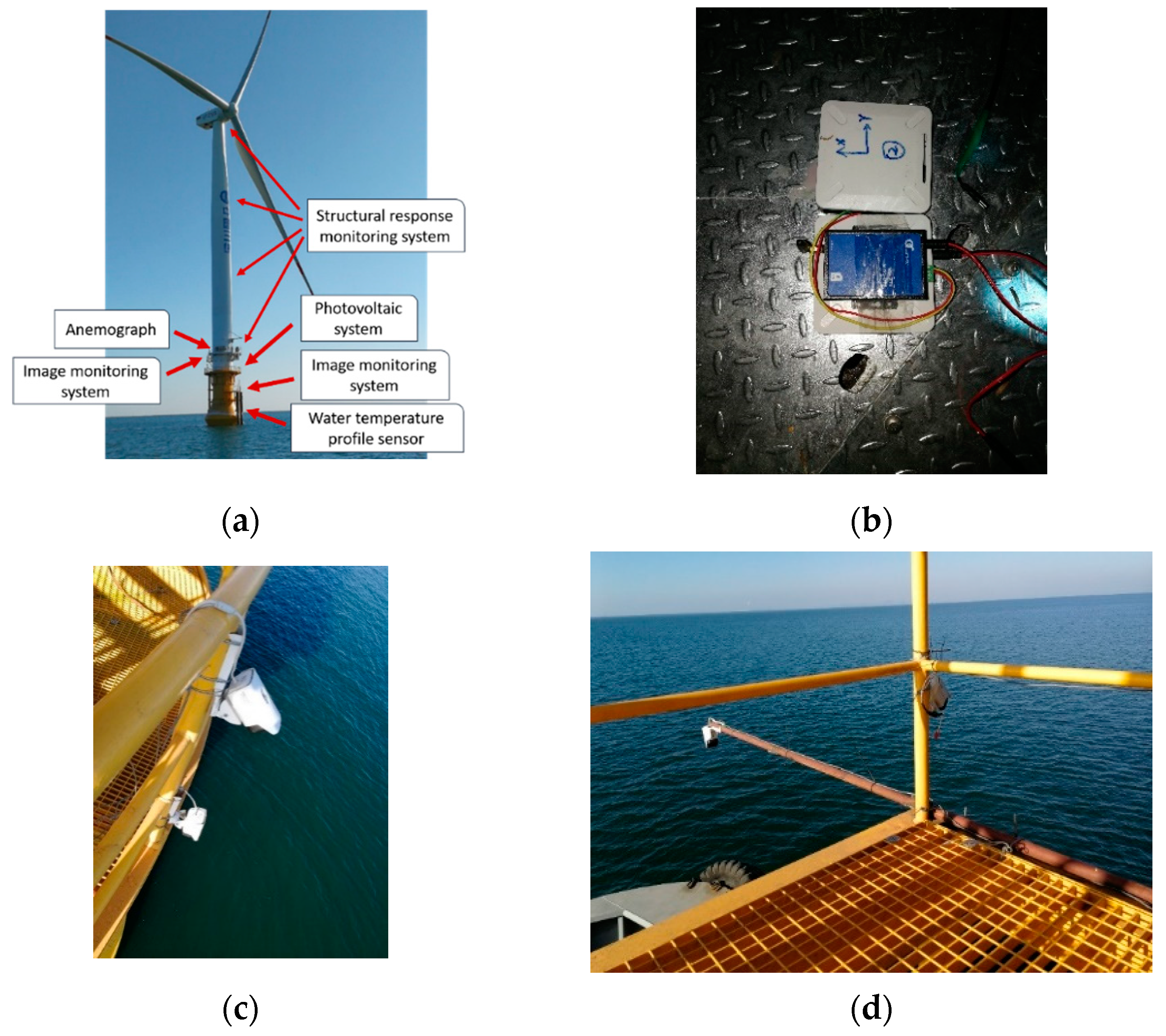
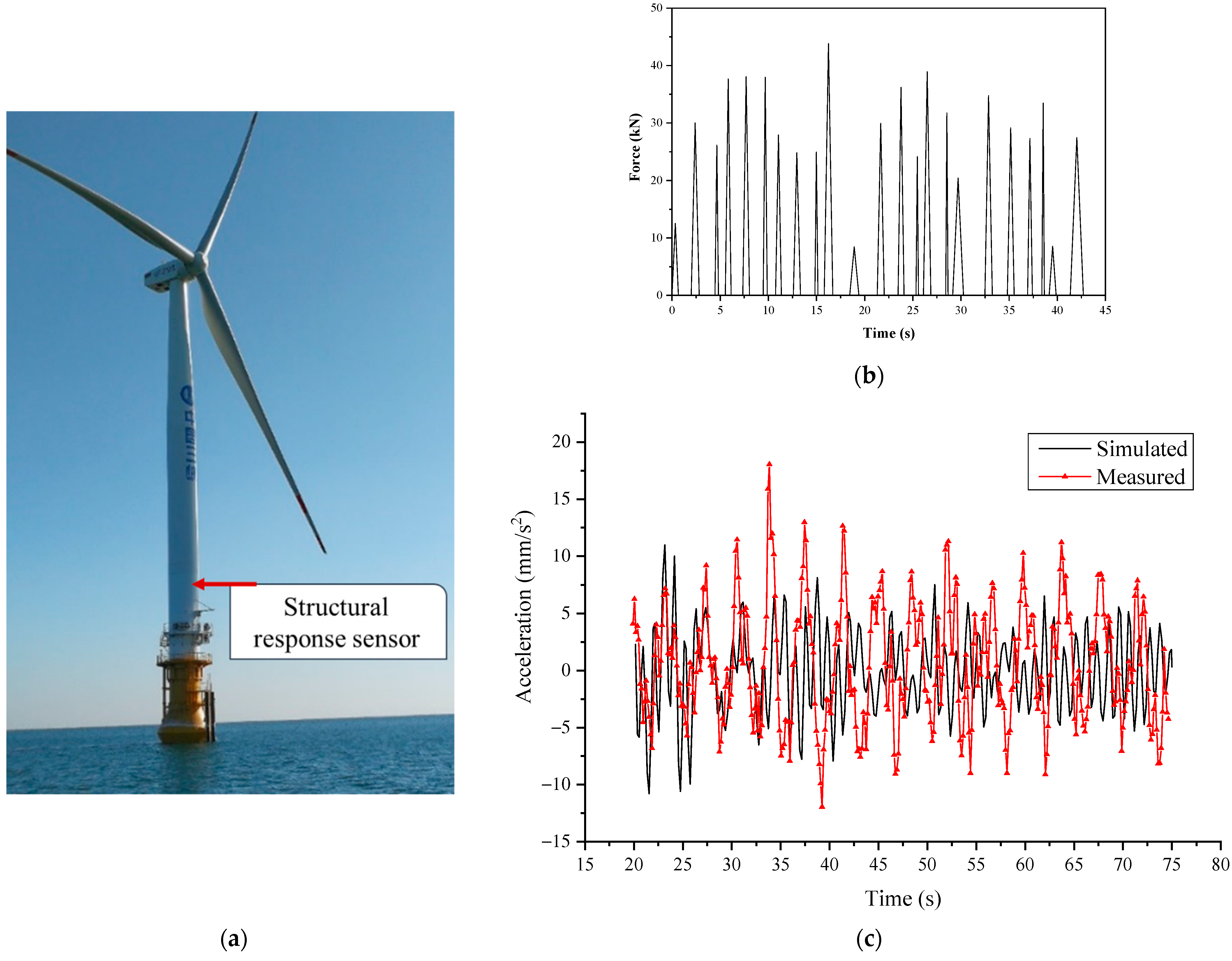
2. Field Monitoring of an OWT in Ice Regions

To obtain data on sea ice conditions, ice load, hydrology and structural response, a field monitoring system was installed on an OWT in the Zhuanghe sea area in the North Yellow Sea of China in the winter of 2017–2018 (39°32.5′ N, 123°19′ E). The structure is a monopile foundation OWT, and a forward and backward ice-breaking cone was installed at the waterline. Its basic properties are shown in

Table 1. Basic properties of the OWT structure.

OWT	Parameters
Top mass	218 t
Tower length	79 m
Tower thickness	0.014~0.039 m
Waterline Diameter	5.5 m
Foundation Thickness	0.065~0.07 m
Ice-breaking cone diameter	9.2 m
Water depth	19 m

. The field monitoring system (FMS) consists of structural-response monitoring system and a sea-ice-conditions monitoring system. The integrated monitoring system of OWT foundations is shown in Figure 1a.

The structural-response monitoring system consists of four sets of acceleration tilt sensors (Figure 1b), and the sea-ice-conditions monitoring system consists of two sets of ice-image cameras (Figure 1c,d, model number: DS-2CD2T86FWDV2-I5S). The cameras conform to the main current direction at 180-degree angles from each other. Each system includes two cameras: the first set for monitoring the ice speed and ice conditions, and the second set for monitoring the ice thickness and ice breaking.

The ice thickness and ice velocity data were obtained from the cameras based on the broken ice pieces that had turned over. The exposed section can be captured by a camera, as shown in Figure 2. The yellow part is the ice-broken cone of the OWT.

By calibrating the camera with fixed focal lengths with an object of a known size, the ratio n is obtained, which relates the length of the object being measured, S, to the pixel length on the image, s, as follows:

$$n=\frac{S}{s}$$

(1)

Then, the expression of the measured ice thickness h and ice speed v is obtained as follows:

$$h=n\times h\prime$$

(2)

$$v=\frac{L}{t}=\frac{n\times l}{t}$$

(3)

where L is the ice breaking length, $h\prime$ and l are the pixel length of ice thickness and ice breaking length on the image, and t is the time that ice takes to pass the breaking length.

During the monitoring period, the level ice lasted for 15 days. It began on 25 January and ended on 8 February of 2018. Only the images with level ice were selected for analysis. The sea ice thickness and sea ice velocity were obtained by collecting multiple sets of data on a group of images and taking the mean value. The maximum level ice thickness measured was 14.9 cm, and the maximum level ice velocity measured was 74.8 cm/s (as shown in Figure 3 and Figure 4).

3. Results

3.1. Deterministic Ice Force Function

Based on long-term monitoring of the Bohai conical jacket platform, Yue et al. established an ice load model for a cone-shaped structure, namely, a deterministic ice force function [16]. The ice force duration is simplified into the form of a right-angled trigonometric function of equal-period amplitudes (Figure 5). This load model assumes that sea ice has the same physical and mechanical properties in the loading section and simultaneously pulses the ice force in each cycle. The peak is used as the starting point of the cycle. In a very short loading time, the sea ice reaches its breaking strength, and the ice force then begins to gradually unload to zero. According to the conclusions obtained from the analysis of measured data of the Bohai oil and gas platform by Yue and Bi [16], as well as Ji and Yue [21], the unloading period of the ice force is 1/3 of the full ice force cycle.

According to experimental analysis, Li and Yue found that the bending fracture length of sea ice is mainly controlled by the sea ice thickness, and the two can be expressed as a linear relationship [22].

$$k=\frac{L}{h}$$

(4)

where L is the length of the sea ice break, h is the ice thickness and k is the ratio of the ice-break length to the ice thickness, which is referred to as the long-thickness ratio coefficient.

Through an analysis of the ice-image data obtained from this field monitoring system, the ice thickness h, length of the sea ice break L and the ratio k were calculated according to the method above. The main data are shown in

Table 2. The sea ice information measured from conical OWT.

h	L	k	h	L	k
cm	cm	-	cm	cm	-
5.41	62.26	11.51	8.49	93.69	11.03
5.87	40.11	6.83	8.51	101.64	11.94
6.51	62.55	9.61	8.84	94.51	10.69
6.52	68.53	10.51	9.18	100.39	10.94
6.76	65.31	9.66	9.23	83.54	9.05
6.87	52.81	7.69	9.37	68.25	7.28
7.14	88.96	12.47	9.76	107.33	10.99
7.17	81.37	11.35	9.82	65.91	6.71
7.17	64.26	8.96	9.82	68.31	6.96
7.17	71.91	10.03	10.01	93.95	9.39
7.20	73.84	10.26	10.01	116.97	11.69
7.24	83.33	11.50	10.01	82.01	8.20
7.31	63.26	8.66	10.44	75.53	7.24
7.39	66.78	9.04	10.44	112.82	10.81
7.47	79.56	10.66	10.47	87.00	8.31
7.84	65.24	8.32	10.57	75.52	7.14
7.84	60.53	7.72	10.57	105.21	9.95
7.95	84.71	10.66	10.64	70.65	6.64
7.95	61.46	7.73	11.21	122.11	10.89
7.95	50.55	6.36	11.72	71.82	6.13
8.11	79.50	9.80	12.80	98.24	7.68
8.28	70.35	8.49	14.90	123.67	8.30

.

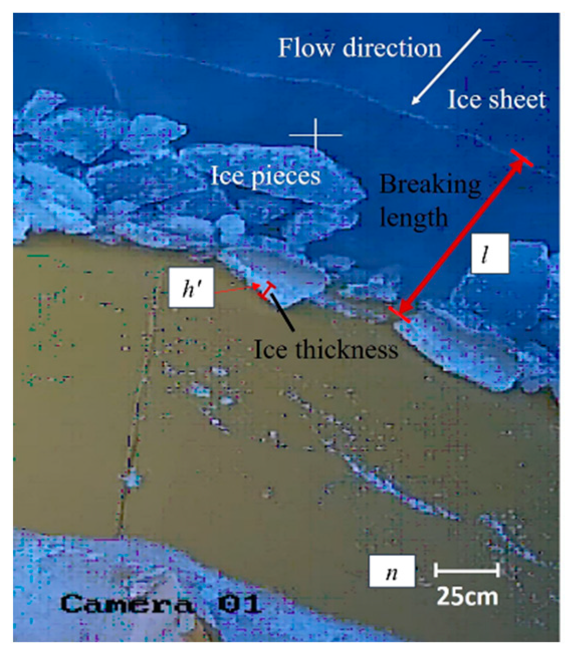
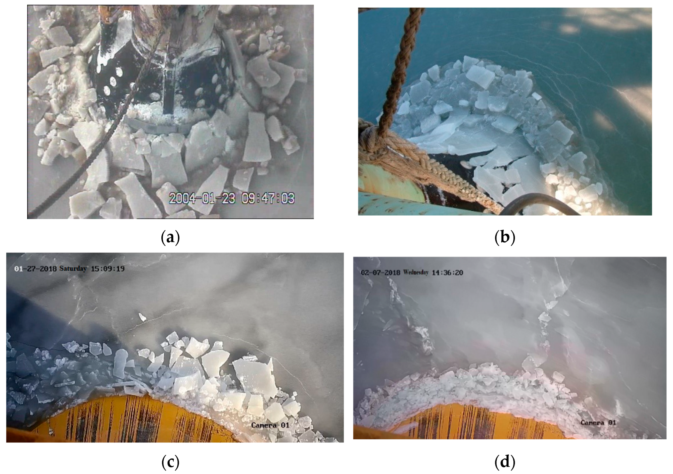
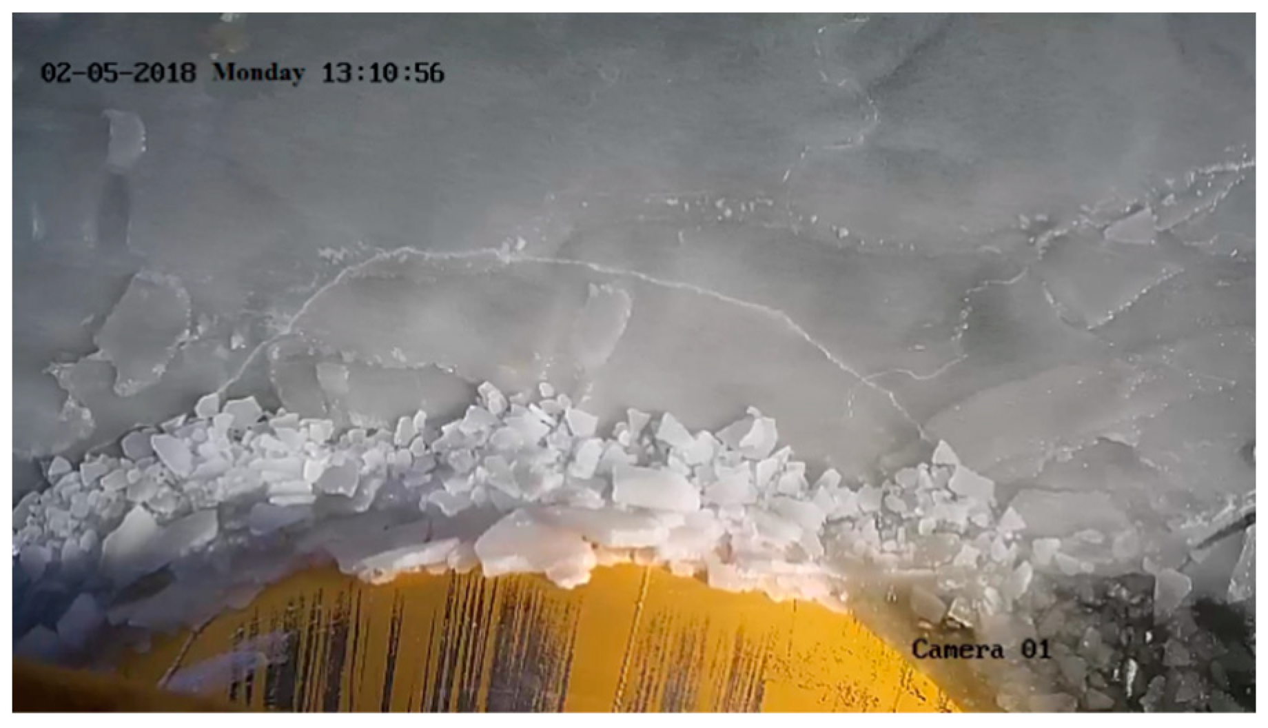
3.2. Sea Ice Breaking Characteristics of Conical Structure

Because the physical and mechanical properties of sea ice exhibit a certain degree of randomness, the fragmentation of sea ice is non-simultaneous on a wider cone structure. Additionally, the greater the width of a structure, and the thinner the sea ice, the more irregular broken ice is. As shown in Figure 6, when the ratio of the diameter of the cone structure to the ice thickness (the ratio of diameter to thickness) increases, the size of the sea ice fracture decreases, and sea ice breaking occurs more non-simultaneously (photos of a and b were taken from JZ20-2MUQ in the Bohai Sea [17], and photos of c and d were taken from an OWT in the Zhuanghe sea area). Therefore, to more accurately simulate ice forces on conical OWTs, it is necessary to analyze the randomness of the ice load.

From on-site image data processing of a conical OWT, sea ice breaking undergoes three stages during the bending failure process: sea ice from the contact cone to the stage of bending failure (ice loading stage), and the broken ice climbs along the cone due to pushing by the subsequent ice plates. The thrust of the subsequent ice plates on the broken ice becomes increasingly smaller (ice force unloading stage). At the same time, the surface on the cone is relatively smooth, and the friction is small. It can be considered that the ice force unloads to 0; the broken ice slides away from both sides of the cone, and the subsequent ice plate has not yet been in contact with the surface of the cone; the ice force is 0 during this period. The fracture characteristics of the sea ice in front of OWTs were the same as those of the sea ice in front of jacket structures in Bohai.

Based on the ice force measurement data of the pressure box of the Bohai conical jacket structure, Qu et al. proposed a model of the random ice force function which simplified the cone ice load into an isosceles triangle with random peaks and periodic distributions [19]. In this function, the time from loading to unloading of the ice forces is 1/3 of the entire period (as shown in Figure 7).

The ice force function throughout one cycle is defined by:

$$f_i(t)=\{\begin{array}{ll}\frac{6F_{0i}}{T_i}t& 0<t<\frac{T_i}{6}\\ 2F_{0i}-\frac{6F_{0i}}{T_i}t& \frac{T_i}{6}<t<\frac{T_i}{3}\\ 0& \frac{T_i}{3}<t<T_i\end{array}$$

(5)

where T_i is the i-th ice force cycle size and F_0i is the ice force amplitude in the cycle. On the basis of Equation (5), a random ice force function of any length of time can be extended:

$$F(t)={\displaystyle \sum _{i=1}^N{f}_i(t-t_i{}^0)}$$

(6)

where N represents the number of ice cycles that need to be established. When i = 0, $t_1{}^0=0$ and when i > 1, $t_i^0={\displaystyle \sum _{j=1}^{i-1}{T}_i}$. When the ice force period is expanded to N, the ice force amplitude is F_0i for each period, and the ice force period T_i constitutes two random series. To obtain a random ice force function that can be applied, it is necessary to calculate the ice force period and ice force amplitude of the real ice force and determine the random distribution of the ice force period and amplitude sequence used in Equation (1).

Based on the measured data of the Bohai platform, the statistical characteristics of the ice force amplitude and ice force period of the cone ice force were analyzed. It was found that both the ice force period and the ice force amplitude obeyed normal distributions, as shown in Figure 8 and Figure 9.

For the ice cycle sequence $T_i~N(\overline{T},{\sigma }_T^2)$, the probability density function can be expressed as:

$$p_T=f(T,\overline{T},{\sigma }_T)=\frac{1}{\sigma \sqrt{2\pi }}{e}^{-\frac{{(T-\overline{T})}^2}{2{\sigma }_T{}^2}}$$

(7)

For the ice force amplitude $F_i~N(\overline{F},{\sigma }_{{}_F}^2)$, the probability density function can be expressed as:

$$p_F=f(F,\overline{F},{\sigma }_F)=\frac{1}{\sigma \sqrt{2\pi }}{e}^{-\frac{{(F-\overline{F})}^2}{2{\sigma }_F{}^2}}$$

(8)

Based on the study by Qu et al. [19], the standard deviation of ice forces is usually 40 to 70% of the average value during the ice cycle. An average of 0.5 can be taken as the value of the standard deviation in the application.

$${\sigma }_T=0.5\overline{T}$$

(9)

At the same time, the coefficients of the variations in ice force amplitudes are randomly distributed between 0.2 and 0.6, and the average value is approximately 0.4. In this application, the standard deviation of the ice force amplitude was considered to be 0.4 times the average value of the ice force, as shown in Equation (10):

$${\sigma }_F=0.4\overline{F}$$

(10)

4. Discussion

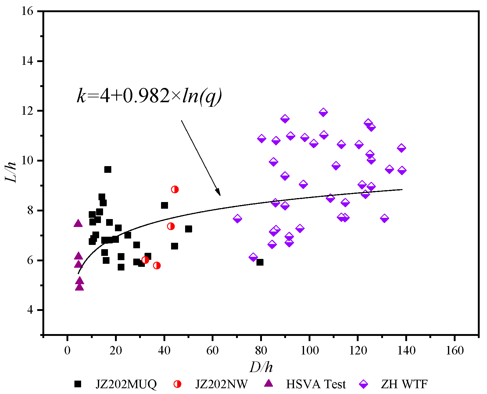
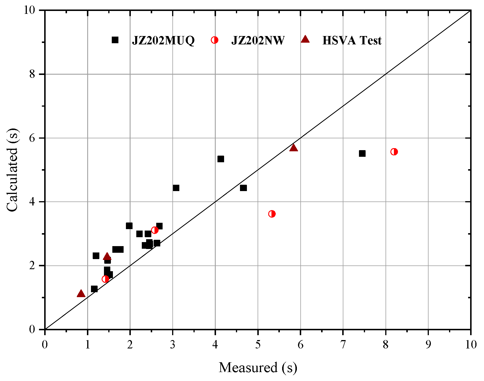
4.1. Average Period of Ice Force

To predict the ice load model suitable for conical OWT, the ice breaking features caused by different conical structures were analyzed. The ice force period, T, is the ratio of ice breaking length L to the ice speed v, which is expressed as follows:

$$T=\frac{L}{v}$$

(11)

Based on field-measured and laboratory test data (as shown in

Table 3. Structural characteristics of different anti-ice cones and their length–thickness ratios, k.

	FF (Hz)	WS (N·m−1)	MCD (m)	k
JZ20-2 MUQ	0.87	4.5 × 107	4	7.16
JZ20-2 NW	1	2.54 × 107	6	6.28
HSVA-Test	-	-	0.61	5.29
ZH-WTF	0.2–0.3	2.66 × 107	9.2	9.19

FF—first-order frequency; WS—waterline stiffness; and MCD—maximum cone diameter; k—length–thickness ratio.

), it can be seen that the aspect ratios of structures with different scales were different. Moreover, these ratios generally increased with increased cone diameters (Figure 10). This is because as the diameter of the cone increased, the linear width of the ice plate thickness increased. At the same time, the length of sea ice breaks and the dispersion of the length of the fracture increased (ice thicknesses were from 5 cm to 40 cm).

Since the cone width influences the length-to-thickness ratio coefficient obtained by fitting, Xu introduced a dimensionless parameter, the width-to-thickness ratio (D/h), in the analysis of ice cones (the ratio of diameter D of the cone at the sea ice to the thickness of sea ice h) [17]; the coefficient q = D/h; therefore, this coefficient was used to analyze the variation law of the aspect ratio. Through video data analysis, it was found that when sea ice acted on a wind-resistant anti-ice cone, when the ice thickness was less than 5 cm, the sea ice breakage length was more dispersed; multiple fractures occurred and were broken into small ice cubes, or splitting damage occurred. Therefore, the measurement data for q < 160 were selected for analysis.

Through an analysis of the data, it was found that coefficient k grew more rapidly with the aspect ratio when the width-to-thickness ratio q was smaller, and the width–thickness ratio grew more slowly when the aspect ratio q was larger (Figure 11). Therefore, the logarithmic form of the equation was used for analysis:

$$k=a+b\ln (q)$$

(12)

From the analysis of the measured data, it was found that the length–thickness ratio coefficient, k, was greater than 4, and the length–thickness ratio coefficient, k, on the cone, which is recommended in ISO19906 [23], ranged from 4~10. Therefore, we used a = 4 in the formula and obtained the relationship between the length–thickness ratio coefficient, k, and the width–thickness ratio coefficient, q, from the measured data; thus, the relationship between the average period of sea ice breaking and ice thickness and ice speed can be obtained:

$$k=4+0.982\ln (q)$$

(13)

$$\overline{T}=\frac{kh}{v}$$

(14)

Based on the ice thickness and ice speed data obtained from field measurements, the ice force cycle was calculated by using the above-described average ice force period relationship, and the measured ice force cycle was compared and analyzed (Figure 12). The overall calculated average period was slightly longer than the measured ice force period. Sea ice inhomogeneity and secondary fractures cause the extracted ice force cycle to be shorter. The measured ice force cycle was based on pressure box data analysis, and the ice thickness and ice velocity were obtained from ice-image cameras. During the climbing process of sea ice interacting on the conical structure, secondary fractures may occur. The period of secondary fracture is less than the primary failure period of sea ice. The period measured by the ice load measured panel includes the period of secondary fracture. Then, compared with the structural response caused by the primary fracture of sea ice, the structural response caused by the secondary fracture of sea ice climbing is small, and the fatigue damage to the structure is also small. The above expression was used to calculate the average ice force cycle to meet engineering needs.

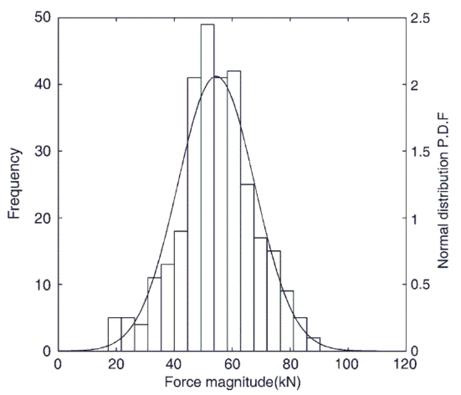
4.2. Ice Force Amplitude

The average ice force, $\overline{F}$, of sea ice is related to the extreme ice force. Qu et al. obtained $\overline{F}=F_{\max }/1.8$ from a statistical analysis of measured data. F_max is the extreme static force on the ice breaking cone [19]. Xu [17], Li and Yue [22], as well as Yu [24] and other scholars, studied the extreme static ice load model on conical structures and analyzed the applicability of the existing static ice load model on the conical platform in Bohai. By contrast, the empirical formula for the total horizontal component of ice breaking derived by Hirayama and Obara (1986) was applied to the narrower cone structure extreme ice load analysis [12]:

$$F_{\max }=B{\sigma }_f{h}^2{(\frac{D}{L_c})}^{0.34}$$

(15)

where ${\sigma }_f$ is the sea ice bending strength, the average bending strength is 750 kPa, h is the sea ice thickness, D is the diameter of the cone structure at the level of ice action and B is an empirical coefficient that takes 3.7 in this paper. L_c is the characteristic length of broken ice, $L_c={(\frac{E{h}^3}{12\rho g})}^{0.25}$; E is the elastic modulus, and its recommended value is 1.5 GPa; ρ is the seawater density, 1.025 kg·m⁻³; and g is the gravitational acceleration, 9.8 m·s⁻².

4.3. Dynamic Ice Load Analysis of Conical OWT

To further analyze the rationality of the ice load model, the OWT measured in the Zhuanghe sea area was simulated numerically. The structure is a monopile foundation OWT, and a forward and backward ice-breaking cone was installed at the waterline. Its basic properties are shown in Table 1. The results of the measurement and simulation were compared to clarify the applicability of the ice load model to OWTs.

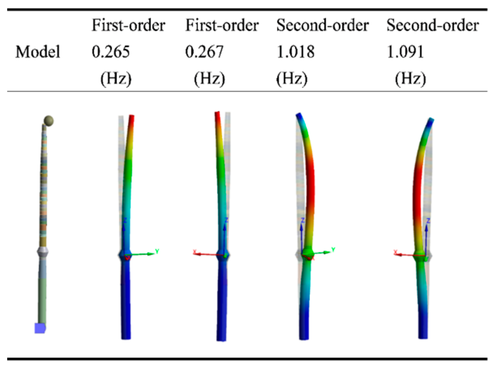
4.3.1. Characteristics of the OWT

According to the properties of the OWT structure in Table 1, a simplified OWT model was established based on the ANSYS finite element software. The tower and foundation were simulated by shell181 elements, and the turbine was simulated by an MASS21 element. By adjusting the model grid, the mesh size was 0.2 m, which can meet the requirements of calculation accuracy and efficiency. The equivalent embedded constraint was used to simulate the constraint of the foundation below mud surface of the OWT. The equivalent pile length of the FEM model is five times that of the pile diameter. The FEM model and modal analysis results of the OWT are shown in Figure 13.

The first-order mode of the OWT swings in the directions of the X-axis and Y-axis, and the natural frequency is approximately 0.265 Hz. The calculated first frequency was close to the actual frequency (0.26 Hz), and the second frequency was approximately 1.02 Hz.

The dynamic characteristics of a structure are determined by mass, stiffness and damping. However, it is difficult to determine the real damping characteristics of a complex structure. The equivalent viscous damping ratio ζ, with the same attenuation rate under free vibration, is typically used to represent structural damping. According to the measured attenuation curve of OWT free vibrations, the damping ratio of the structure calculated by the logarithmic reduction method was approximately 0.02. The Rayleigh damping model is often used in vibration analysis in ANSYS. It was assumed that the damping matrix of the structure was a linear combination of the mass matrix and stiffness matrix ($C=\alpha M+\beta K$). In this expression, α is the mass damping coefficient, and β is the stiffness damping coefficient. The i-th modal damping ratio ζ_i can be expressed as:

$${\mathsf{\zeta }}_i=\frac{C_i}{2\sqrt{M_i{K}_i}}=\frac{\alpha M_i+\beta K_i}{2\sqrt{M_i{K}_i}}=\frac{1}{2}(\frac{\alpha }{{\omega }_i}+\beta {\omega }_i)$$

(16)

Because the first-order vibration characteristics of OWTs are mainly considered under the action of sea ice, the first two natural frequencies were mainly analyzed. According to the analysis of the measured data, the damping ratio of the structure was 0.02. Then, the parameters α and β were calculated.

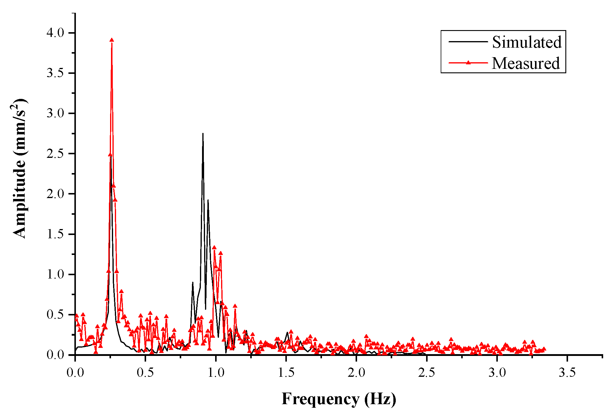
4.3.2. Verification of the Random Ice Load Model of the OWT

To measure the coupling effect between sea ice and other environmental loads, the structural-response monitoring system consisted of four sets of acceleration tilt sensors which were evenly distributed inside the tower from the top. The X-axes of the sensors were parallel to the main ice direction. For the monitoring of sea ice conditions and ice breaking, image monitoring methods using two sets of ice-imaging cameras were adopted. Through the analyses of the monitoring data, we extracted data from a day when the wind speed was low (lower than moderate breeze) and ice conditions were serious. At 13:10 on that day, the average ice thickness was 0.11 m, and the ice velocity was 0.51 m·s⁻¹ (Figure 14).

From the above analysis of ice periods and ice amplitudes, the random ice force of a conical OWT can be established. Based on the Monte Carlo method, a time history simulation of random ice forces on a conical OWT using the MATLAB software (Figure 15b) was conducted; the ice force time history data were applied to the ANSYS FEM of the OWT to analyze the structural response. An acceleration sensor was located in the tower and 14 m from the top of the foundation (Figure 15a). The acceleration response data of the structure corresponding to the sensor placement point in the FEM were extracted.

From the comparison between the measured acceleration and the simulated acceleration time history curves in Figure 15c, it was found that the measured values of the acceleration amplitudes were slightly larger than the simulated values. As shown in

Table 4. Acceleration and period comparison between simulation and measurement.

	astd (mm·s−2)	amax (mm·s−2)	Tave (s)	Tstd (s)
Simulated	3.61	10.98	1.52	0.35
Measured	4.91	11.30	1.88	0.36
Error (%)	26.6	2.8	19.1	2.8

a_std—standard deviation of acceleration; a_max—maximum acceleration; T_ave—average period; T_std—standard deviation of period.

, the maximum measured acceleration was 11.3 mm·s⁻², and that from the simulation was 10.98 mm·s⁻². The error between the two was 2.8%. In comparing the acceleration standard deviation of the measurement and the simulation, it is found that the error between them was 26.6%. By comparing the acceleration data, the maximum acceleration difference between the simulated value and the measured value was small, and the standard deviation had some errors. The average period of the simulated values was 1.52 s, and the average period of the measured values was 1.88 s. The error between them was 19.1%. The standard deviation error between the simulated value and the measured value was 2.8%. Because the influence of wind loads was not considered in the numerical simulation, the measured values were influenced by the wind load. Therefore, there were some errors between the amplitudes and the average periods in the measured and simulated values.

To further analyze the correlation between the measured and the simulated values and clarify the corresponding relationship between them in the frequency domain, the acceleration data were transformed with a Fourier transform. Fourier transforms can establish the conversion relationship between time-domain signals and frequency-domain signals and can reflect the proportion of signals at different frequencies. The fast Fourier transform (FFT) is a fast algorithm of the Fourier transform. The relationship between the amplitude and the frequency components of the acceleration data was obtained by FFT processing of the simulated and measured data. The comparative analysis results are shown in Figure 16.

Figure 16 shows that the simulated values and the measured data had similar amplitude–frequency relationship curves and that the amplitude responses were concentrated at approximately 0.25 Hz and 1.0 Hz. By comparing the frequencies corresponding to the first three highest peaks (as shown in

Table 5. Comparison of peak frequency between simulated value and measured value.

	First Peak Frequency (Hz)	Second Peak Frequency (Hz)	Third Peak Frequency (Hz)
Simulated	0.251	0.907	0.951
Measured	0.262	0.988	1.042
Error (%)	4.2	8.2	8.8

), the first peak frequency of simulation was 0.251 Hz, and that of measurement was 0.262 Hz. The error between the measured and the simulated value was 4.2%. In comparing the next two peak frequencies of the simulated value and the measured value, it was found that the errors between them were 8.2% and 8.8%. The errors were relatively small. The amplitude responses of the numerically simulated accelerations were similar at both frequencies. The amplitude response of the measured accelerations was mainly concentrated at 0.25 Hz, and there was a corresponding peak near 1.0 Hz. Different from the measured data, which were affected by other environmental conditions such as winds and currents, the numerical simulation only considered the influence of sea ice loads; there were thus some differences in the amplitude responses between the two, but the overall response trends were the same.

Based on the above analysis, the formulas for the average periodic ice forces and for random ice forces are suitable for conical OWT structures.

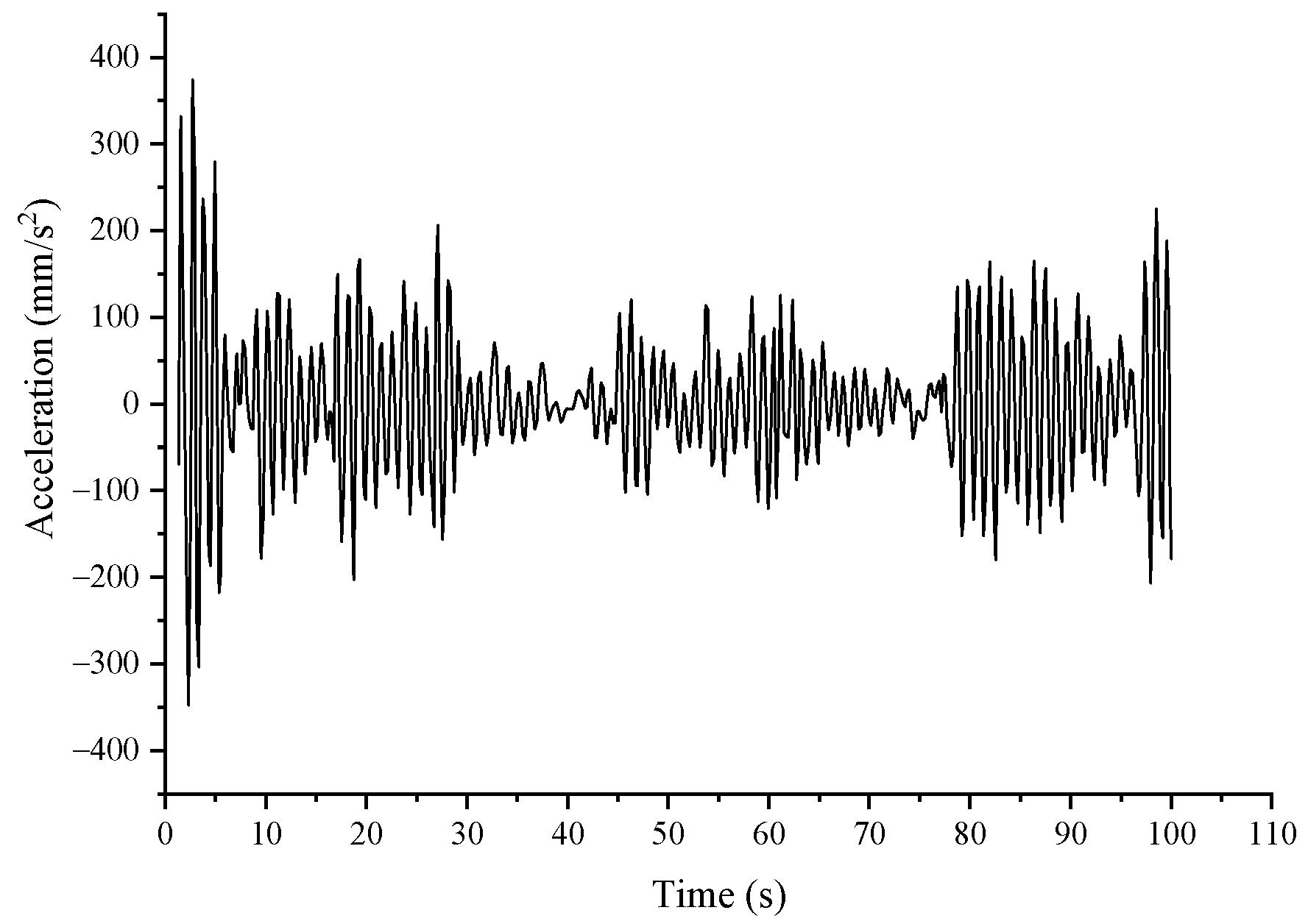
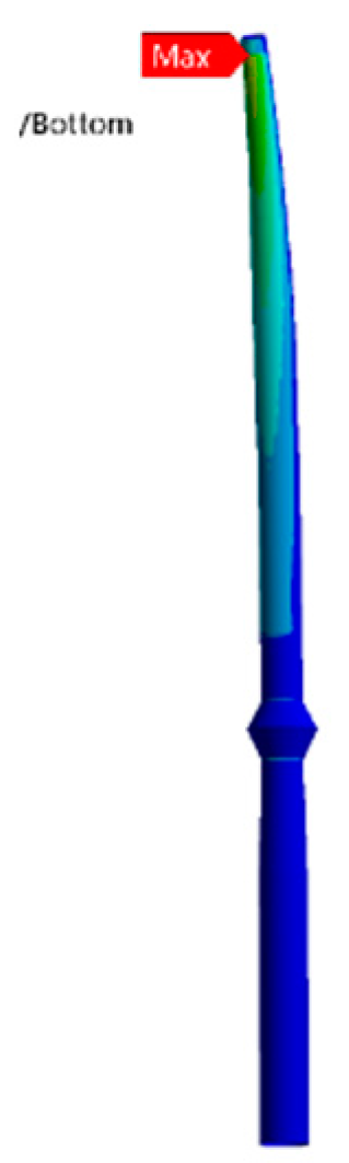
4.3.3. Ice-Induced Vibration of the OWT

The ultimate ice thickness in the wind farm was 0.32 m (50-year return period). Due to the lack of long-term distribution data for ice velocities, the ice speed data measured in that year were used as the analysis data for ice velocities. The measured maximum ice velocity was 0.75 m·s⁻¹. The ice load may induce resonance when the ice breaking period is close to the natural period of the structure where the natural period is 3.77 s. The ice velocity was 0.63 m·s⁻¹, which was calculated using Equations (13) and (14) in Section 4, when the ice thickness was 0.32 m. The numerical simulation of the structural response was based on the two ice conditions (as shown in

Table 6. The design ice load for the simulation.

IC	Thickness (m)	Velocity (m·s−1)	Period (s)
RIC	0.32	0.63	3.77
UIC	0.32	0.75	3.17

IC—ice conditions; RIC—resonant ice conditions; UIC—ultimate ice conditions.

).

The numerical simulation curves in Figure 17 and Figure 18 show that there was no resonance in the structural response curve at the hub when the average ice force period was equal to the first natural period of the structure, and the acceleration curve characteristics and amplitude were similar to those under ultimate ice conditions. On the one hand, because the ice velocities of the two were close and the ice velocity was relatively high, the ice force periods were relatively close, and the extreme ice forces of the two were the same; thus, the vibration responses of the structure were relatively close. On the other hand, when the ice force period was close to the structural period, the resonance amplification phenomenon of the structure response was not induced, and the vibration of the structure still presented randomness. Due to the nonuniformity of natural sea ice, the bending failure of the ice exhibited randomness.

The numerical simulation curves in Figure 19 and Figure 20 show that the acceleration response was random at the top of the foundation (ToF) and that the acceleration curve characteristics and amplitude were similar to those under ultimate ice conditions. The reason was the same as described above.

By comparing Figure 17, Figure 18, Figure 19 and Figure 20, it can be seen that the response at the ToF and at the hub for the two ice conditions exhibited the same trend. The difference was that the acceleration response frequency at the ToF was higher than that at the hub, and the acceleration response at the ToF was similar to that at the hub. However, the displacement response at the ToF was far less than that at the hub (as shown in

Table 7. The responses of the OWT under UIC and RIC.

IC	Hub		ToF
	MD (mm)	MA (mm·s−2)	MD (mm)	MA (mm·s−2)
RIC	253	319	32	374
UIC	237	323	27	313

IC—ice conditions; RIC—resonant ice conditions; UIC—ultimate ice conditions; MD—maximum displacement; and MA—maximum acceleration.

). The vibration acceleration at the ToF should be considered for OWTs in cold regions.

After transient analysis, the responses with large von Mises stress and the largest amplitude changes were defined as hot spot stress. It can be seen from the hot spot stress positions (Figure 21 and Figure 22) and stress curves (Figure 23 and Figure 24) that the hot spot stress position was the same under resonant ice conditions (RIC) and ultimate ice conditions (UIC); the maximum stress was 116.4 MPa under RIC, and the maximum stress was 116.1 MPa under UIC. The stress results were calculated using the rain flow counting method. These results showed that the maximum stress amplitude was 37.7 MPa and the corresponding average stress was 97.5 MPa under RIC; the maximum stress amplitude was 35.6 MPa and the corresponding average stress was 97.5 MPa under UIC (shown in

Table 8. OWT fatigue limits under ice conditions.

IC	Sa (MPa)	Sm (MPa)	Su (MPa)	S−1 (MPa)	FL (MPa)
RIC	37.7	97.5	600	44.8	37.3
UIC	35.6	97.5	600	42.5	37.3

S_a—stress amplitude; S_m—average stress; S_u—maximum strength; S_−l—equivalent fatigue stress; and FL—fatigue limit. All variables were 10⁸ cycles.

).

$$(S_a/S_{-1})+(S_m/S_u)=1$$

(17)

Based on the Goodman linear formula (Equation (17)), the corresponding fatigue limit can be calculated (as shown in Table 7). According to the S-N curve recommended in DNV-Os-J101 [25], the fatigue limit for 10⁸ cycles is 37.3 MPa. Fatigue damage to the structure can be caused by sea ice. It is necessary to evaluate fatigue damage to OWTs in cold regions.

5. Conclusions

Based on the monitoring of conical OWTs in cold regions, the length and characteristics of sea ice breaking on conical OWTs were obtained. Sea ice breaking on conical structures is random; therefore, the ice load is random. According to data analysis, the key parameters of dynamic ice loads are the average ice force period and the ice force amplitude.

It was determined that the mean ice force period and ice force amplitude obeyed normal distributions. Based on the analysis of the field measurement data of different-sized conical structures, the formula for the average ice force period was established. By comparing the measured period data with the calculated period data, it was found that the error between the two was small and could be used to calculate the ice force period.

A prediction model of ice forces for conical OWTs was established in this paper. By comparing the structural responses of the numerically simulated and measured data, it was found that both were consistent in the time and frequency domains. It was verified that the established ice force model is suitable for conical OWT structures.

When the average ice force period is equal to the natural period of the structure, the vibration response of the structure still presents random vibration characteristics without resonance amplification. The vibration acceleration at the ToF should be considered for OWTs in cold regions. Sea ice can cause fatigue damage to OWTs at the hot spot located in the upper part of the tower. It is necessary to evaluate ice-induced fatigue damage to OWTs.

References

1. Guojun, W.; Dayong, Z.; Chunjuan, L. Vibration analysis of offshore wind turbine foundation in ice zone. Ship Ocean Eng. 2016, 45, 109–113. [Google Scholar] [CrossRef]
2. Chunjuan, L. Study on the Design of Simple Offshore Wind Turbine Foundation; Dalian University of Technology: Dalian, China, 2017. [Google Scholar]
3. Ye, K.; Li, C.; Yang, Y.; Zhang, W.; Xu, Z. Research on influence of ice-induced vibration on offshore wind turbines. J. Renew. Sustain. Energy. 2019, 11, 1–19. [Google Scholar] [CrossRef]
4. Hendrikse, H.; Seidel, M.; Metrikine, A.; Løset, S. Initial results of a study into the estimation of the development of frequency lock-in for offshore structures subjected to ice loading. In Proceedings of the 24th International Conference on Port and Ocean Engineering under Arctic Conditions, Busan, Korea, 11–16 June 2017. [Google Scholar]
5. Seidel, M.; Hendrikse, H. Analytical assessment of sea ice-induced frequency lock-in for offshore wind turbine monopoles. Mar. Struct. 2018, 60, 87–100. [Google Scholar] [CrossRef] [Green Version]
6. Q/HSn 3000-2002; Regulations for Offshore Ice Condition & Application in China Sea. CNOOC: Beijing, China, 2002.
7. Yue, Q.; Xu, N.; Cui, H.; Ma, C.J. Effect of adding cone to mitigate ice-induced vibration. Ocean Eng. 2011, 29, 18–24. [Google Scholar] [CrossRef]
8. Lavoie, N.Y. Ice effects on structures in the Northumberland Strait crossing. In Ice Pressures against Structures, NRC Technical Memo No. 92; (NRC No. 985); Department of Fisheries and Oceans, Department of Transport: Ottawa, ON, Canada, 1966. [Google Scholar]
9. Croasdale, K.R.; Cammaert, A.B.; Metge, M. A method for the calculation of sheet ice loads on sloping structures. In Proceedings of the 12th International Symposium on Ice, Trondheim, Norway, 23–26 August 1994. [Google Scholar]
10. Ralston, T.D. Ice force design considerations for conical offshore structures. In Proceedings of the 4th International Conference on Port and Ocean Engineering under Arctic Conditions, St. John’s, NL, Canada, 26–30 September 1977. [Google Scholar]
11. Kato, K. Experimental studies of ice forces on conical structures. In Proceedings of the 8th IAHR Ice symposium, Iowa City, IA, USA, 18–22 August 1986. [Google Scholar]
12. Hirayama, K.; Obara, I. Ice forces on inclined structures. In Proceedings of the 5th International Offshore Mechanics and Arctic Engineering, Tokyo, Japan, 13–18 April 1986. [Google Scholar]
13. Yonghai, Y.; Qianjin, Y. Prediction methods of sheet ice load on conical structures. Acta Oceanol. Sin. 2000, 22, 74–85. (In Chinese) [Google Scholar] [CrossRef]
14. Sodhi, D.S.; Morris, C.E.; Cox, G.F.N. Dynamic analysis of failure modes on ice sheets encountering sloping structures. In Proceedings of the 6th International Conference on Offshore Mechanics and Arctic Engineering, Houston, TX, USA, 1 March 1987. [Google Scholar]
15. Frederking, R. Dynamic ice forces on an inclined structure. In Physics and Mechanics of Ice; Springer: Berlin/Heidelberg, Germany, 1980; pp. 104–116. [Google Scholar]
16. Qianjin, Y.; Xiangjun, B. Ice-induced jacket structure vibrations in Bohai Sea. J. Cold Reg. Eng. 2000, 14, 81–92. [Google Scholar] [CrossRef]
17. Xu, N. Research on Ice Force of Conical Offshore Structures; Dalian University of Technology: Dalian, China, 2011. [Google Scholar]
18. Qianjin, Y.; Xianjun, B.; Xiao, Y.; Zhongmin, S. Ice-induced vibration and ice force function of conical structure. China Civ. Eng. J. 2003, 36, 16–19. [Google Scholar] [CrossRef]
19. Yan, Q.; Qianjin, Y.; Xiangjun, B.; Tuomo, K. A random ice force model for narrow conical structures. Cold Reg. Sci. Technol. 2006, 45, 148–157. [Google Scholar] [CrossRef]
20. Qianjing, Y.; Yan, Q.; Xiangjun, B. Ice force spectrum on narrow conical structures. Cold Reg. Eng. 2007, 49, 161–169. [Google Scholar] [CrossRef]
21. Shunying, J.; Qianjin, Y. Monte-Carlo simulation of fatigue ice-load for offshore platform with ice-broken cone in the Liaodong Gulf. Acta Oceanol. Sin. 2003, 25, 114–119. [Google Scholar] [CrossRef]
22. Feng, L.; Qianjin, Y. Failure of ice sheet under simultaneously longitudinal and transverse load on slope structures. J. Hydraul. Eng. 2000, 31, 44–48. [Google Scholar] [CrossRef]
23. ISO 19906; Petroleum and Natural Gas Industries-Arctic Offshore Structures. International Standard Organization (ISO): Geneva, Switzerland, 2010.
24. Xiao, Y. Research on Ice Force of Conical Structures in Bohai; Dalian University of Technology: Dalian, China, 2001. [Google Scholar]
25. DNV-Os-J101; Design of Offshore Wind Turbine Structures. Det Norske Veritas: Bærum, Norway, 2014; pp. 129–130.
Figure 1. FMS implementation on an OWT foundation: (a) FMS implementation on an OWT foundation; (b) acceleration tilt sensors; (c) first set of ice-image cameras; (d) second set of ice-image cameras.
Energies 15 03357 g001
Figure 2. Image monitoring methods of sea ice factors.
Energies 15 03357 g002
Figure 3. The maximum level ice thickness measured per day in January and February 2018.
Energies 15 03357 g003
Figure 4. The maximum level ice velocity measured per day in January and February 2018.
Energies 15 03357 g004
Figure 5. Simplified deterministic ice force model of a conical structure.
Energies 15 03357 g005
Figure 6. Sea ice bending failure on cones of different scales: (a) diameter-to-thickness ratio is 20; (b) diameter-to-thickness ratio is 45; (c) diameter-to-thickness ratio is 90; (d) diameter-to-thickness ratio is 180.
Energies 15 03357 g006
Figure 7. Simplified random ice force model on the cone structure.
Energies 15 03357 g007
Figure 8. Normal distribution characteristics of ice periods.
Energies 15 03357 g008
Figure 9. Normal distribution characteristics of flat-ice force amplitudes.
Energies 15 03357 g009
Figure 10. Length–thickness ratios, k, of sea ice bending failures at different scales.
Energies 15 03357 g010
Figure 11. Length–thickness ratio, k, versus the width–thickness ratio, q.
Energies 15 03357 g011
Figure 12. Comparison between the calculated ice force periods and the measured ice force periods.
Energies 15 03357 g012
Figure 13. FEM model and modal analysis results for the OWT.
Energies 15 03357 g013
Figure 14. Bending failure phenomenon of ice on a conical OWT.
Energies 15 03357 g014
Figure 15. (a) Location point of the acceleration sensor; (b) time history curve of random ice forces under typical ice conditions; (c) simulated acceleration versus measured acceleration.
Energies 15 03357 g015
Figure 16. The measured data versus analysis result of acceleration after FFT transformation.
Energies 15 03357 g016
Figure 17. Response accelerations of the hub under resonant ice conditions (ice thickness was 0.32 m and ice velocity was 0.63 m·s−1).
Energies 15 03357 g017
Figure 18. Response accelerations of the hub under ultimate ice conditions (ice thickness was 0.32 m and ice velocity was 0.75 m·s−1).
Energies 15 03357 g018
Figure 19. Response accelerations at the ToF under resonant ice conditions (ice thickness was 0.32 m and ice velocity was 0.63 m·s−1).
Energies 15 03357 g019
Figure 20. Response accelerations at the ToF under ultimate ice conditions (ice thickness was 0.32 m and ice velocity was 0.75 m·s−1).
Energies 15 03357 g020
Figure 21. Hot spot under RIC (ice thickness was 0.32 m and ice velocity was 0.63 m·s−1).
Energies 15 03357 g021
Figure 22. Hot spot under UIC (ice thickness was 0.32 m and ice velocity was 0.75 m·s−1).
Energies 15 03357 g022
Figure 23. Stress at the hot spot under RIC (ice thickness was 0.32 m and ice velocity was 0.63 m·s−1).
Energies 15 03357 g023
Figure 24. Stress at the hot spot under UIC (ice thickness was 0.32 m and ice velocity was 0.63 m·s−1).
Energies 15 03357 g024