1. Introduction
As a result of HSPMSM’s inevitable benefits of high torque density, dynamic performance, and high efficiency [
1,
2,
3,
4], they have become crucial parts of micro-turbines [
5], equipment gas compressors [
6], flywheel energy storage [
7], spindle equipment [
8], turbo-molecular, and pumps [
9]. These reduce emissions and enhance combustion efficiency [
10]. In centrifugal blowers design optimization, the complement to achieving high precision, engineers have focused on developing a lightweight and more compact design with high efficiency and high torque density. An electric machine’s higher torque density is limited by three factors: mechanical, electromagnetic, and thermal limit [
11]. The mechanical constraint is linked with the strength of mechanical components like shafts and bearings. The magnetic saturation of the electrical steel used to manufacture both stator and rotor cores is connected to the electromagnetic limit. High-performance materials, e.g., high permeability, low-loss soft magnetic materials, and high strength bearings, are the only ways to solve both electromagnetic and mechanical limits.
The electric machine’s thermal limit is represented by the highest temperature rise that insulating materials sustain (i.e., thermal class) [
12]. However, HSPMSMs have special problems because of the high power density that is achieved by supplying a high-frequency current to the stator winding, which causes a significant increase in copper losses. Furthermore, due to the machine’s compact size, heat is concentrated rapidly [
13] without adequate cooling. It might lead to a temperature rise above the safe limit by increasing thermal stress on the electrical insulation of the windings [
14]. Therefore, appropriate heat management can alleviate this thermal constraint, such as forced liquid cooling [
15,
16], thus allowing a machine designer to choose an optimal cooling system.
Although forced radial air-cooling via radial winding holes can reduce winding local overheating and thus protect the winding insulation [
17], this method is more often used for large dissipation areas. The effectiveness of forced air cooling axial ventilation in uniformly distributing temperature via the PMSM axial direction was examined [
18]. However, this method was also useful in cooling the winding ends inside the slot winding.
In this study, in order to meet the requirements of lighter weight and more compact size with high torque density, high efficiency, and lower winding temperature rise for 225 kW HSPMSM to be used in an air suspension centrifugal blower application, an electromagnetic and thermal analysis is conducted considering the axial machine’s length minimization. Firstly, four different analytical models (A2–A5) in the electromagnetic analysis are derived by minimizing the initial machine’s (A1) axial length. The best among analytical models is chosen as the A4 model with lighter weight and more compact structure in addition to higher torque density than A1, A2, and A3 models, and higher efficiency than A1, A2, A3, and A5 models by HSPMSM’s, optimal geometric design, and optimal material choice, respectively. Secondly, LPTN is designed to predict the entire analytical model’s thermal behavior in the thermal analysis. Then, sensitivity analysis for the stator axial ventilation to the cooling performance is investigated, and the parameters scopes are determined. The optimal parameters which generate adequate heat distribution could be obtained by analyzing the effects of stator axial ventilation duct’s width and number on winding temperature rise. Analysis indicates that winding temperature rises from the A4 model is kept much lower than winding insulation via the obtainable optimal axial ventilation parameters. Finally, different analytical models are prototyped and tested. The comparisons between predicted electromagnetic performance, winding temperature rise, and test results were carried out, and results were found to agree with each other consistently.
The organization of this paper is as follows:
Section 1 introduces the literature on electromagnetic and thermal analysis of HSPMSM.
Section 2 gives detail on the electromagnetic analysis of HSPMSM.
Section 3 presents the proposed LPTN considering the airflow and heat transfer mechanisms of HSPMSM with FACAVS.
Section 4 validates experimentation and discussion, and in
Section 5 a conclusion is drawn.
2. Electromagnetic Analysis
2.1. Specification for the Design
An axial machine’s length of 210 mm is chosen as the initial design parameter to meet the needed performance. A single-layer distributed winding model is selected to meet the required factor for slot fill and minimum copper losses. Efficiency is maximized, and cogging torque is minimized.
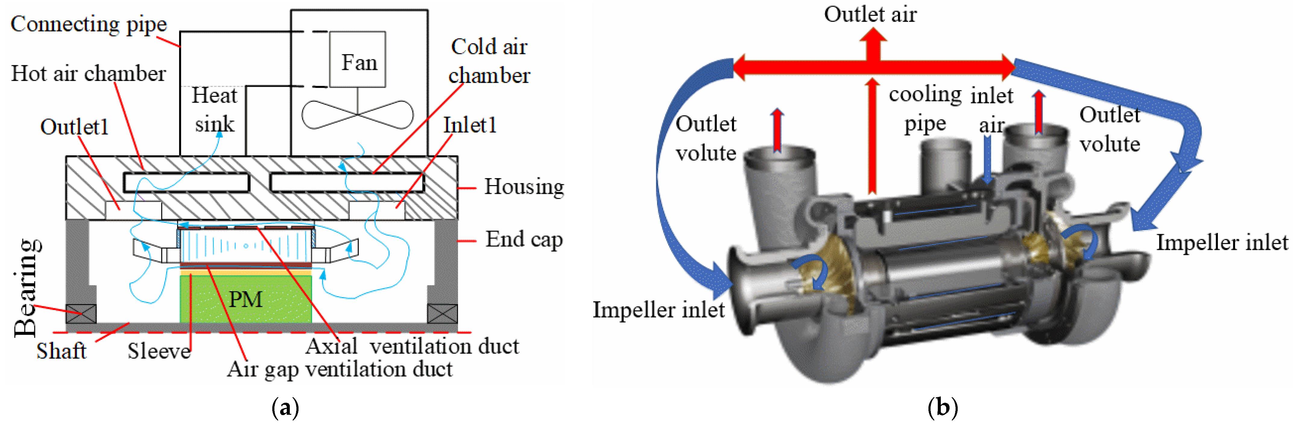
Figure 1 depicts the structure of the 225 kW HSPMSM with FACAVS, where
Figure 1a,b present the 2D cut view with two parallel ventilation ducts, and 3D cut view of the machine with air cooling’s passage, respectively, and
Table 1 presents the design specifications. The derivations of four analytical models are based on the initial model to enhance the performance and minimize the volume of the HSPMSM. The establishments of these models are achieved by minimizing the initial axial machine’s length to meet the design requirements of lighter weight and more compact structure with the following better performances as stated below:
Magnetic machine’s performance: All models should have the same power output. Moreover, torque density and efficiency must be higher or equal to the initial model.
The factor for slot’s fill: turn’s per slot under slot’s fill of less than 54% is increased to cater for an amount of power due to axial machine’s minimization.
Thermal performance: the best analytically derived model should have the highest winding temperature rise below winding’s insulation class (B) to improve the machine’s lifespan.
According to A1, with a 210 mm core length, four different models have been developed analytically (A2, A3, A4, and A5) and achieved turns per slot modification with the corresponding core length are 200 mm, 190 mm, 180 mm, and 170 mm for the A2–A5 models, respectively. An overhang was employed for the PM to maintain the power output of the A5 model. Analytical models are analyzed differently according to varying axial machine lengths; in the model with an overhang (A5), the coefficient of the overhang is taken into consideration by an increase in PM material remanence value that denotes the ratio of electromagnetic performance of an over-hang to non-over-hang. The depth for the A5 model is 170 mm, and
Figure 2a illustrates an analytical machine’s design model.
2.1.1. Optimal Selection of Material
Interior PM and surface-mounted rotors are two rotor alternatives for HSPMSMs. The latter is preferred because it can withstand large stress caused by high-speed rotor rotation. Many HSPMSMs use Sm-Co or Nd-Fe-B as PM material to minimize the influence of the air gap reluctance. The former can adopt higher temperature, but remanence is lower while the latter has better BH characteristics; therefore, it is selected in this paper. The basic HSPMSM’s material thermal properties are given in
Table 2.
Moreover, this study considers high-frequency stator and rotor lamination material to reduce iron losses. Thus, steel Amon 73.5% Si material with a thickness of 0.175 mm is used instead of traditional 0.35 M235-35 material; the comparison of these two-silicon materials is presented in
Table 3. A high-strength composite material for retaining sleeves is needed to protect surface-mounted PM against damage, including glass fiber, carbon fiber, or a special alloy including titanium. However, alloy generates an additional eddy current losses. Therefore, carbon fiber is chosen with the yielding deformation fatigue, high tensile strength, and endurance.
2.1.2. Determination of PM Thickness and Volume
The right electromagnetic load selection is made based on the economic performance and technical requirements of the designed HSPMSM. When the PM thickness is determined, load influence, demagnetization, and temperature must be considered during the heavy load operation of the HSPMSM. Equation (1) determines PM thickness as reported in [
19], and the nomenclature section contains definitions for all of the symbols involved in the equations.
where m is the number of phases,
is the RMS maximum current, N is the number of turn’s,
is the winding factor, P is the pole’s number, and
is the Coercive force.
Considering the maximum power output and volume ratio of the PM when HSPMSM operates at rated load, an analytical method is used to determine PM volume in [
19] by
where
is the demagnetization field intensity,
is the rated electric line load, and
is the density of the PM’s material.
2.1.3. Determination of HSPMSM Geometry
The geometric design of HSPMSM mainly consists of dimensioning the armature length
) and the diameter of the inner stator. The armature length is obtained analytically by taking torque (electromagnetic) and load into account, as presented in [
19]
where
is the maximum electromagnetic torque,
is the fundamental amplitu-de of the air gap’s flux, and
is the inner diameter of the stator.
The HSPMSM’s power and speed are determined according to the given specification’s index performance of electromagnetic load
. The actual dimension is chosen to obtain the actual HSMPM size. Based on dynamic response and electromagnetic load, the inner diameter of the stator is estimated [
19] as
where
is the time starting from linear zero speed to rated angular speed ω and
is the density of the stator’s core material.
The dimension of the stator yoke and teeth are designed to minimize the magnetic reluctance of the HSPMSM. According to the previously determined structure, the stator simplified model is obtained. Therefore, Equation (7) is derived to estimate the overall magnetic reluctance. It is shown in
Figure 3 that the flux becomes distributed symmetrically along bilateral direction inside the stator model, having the starting from the left half of each piece of upper teeth, then pass across the yoke and finally return to the lower teeth.
When we assume that all flux pass across the core, to determine a magnetic reluctance (average) for the teeth and yoke, it becomes compulsory to obtain a path of the flux, which is assumed to be the middle of the core that is drown with the red line as shown in
Figure 3. Equations (5)–(8) can be obtained by taking the magnetic core circuit equivalent to an electric circuit shown in
Figure 3 using the method presented in [
19]
where
is the stator yoke inner diameter,
is the outer diameter of the stator, x is the half-width of the tooth,
is the magnetic reluctance for teeth, and
is the magnetic reluctance for the yoke, and S is the slot’s number.
2.2. Analysis of Power Losses
The primary losses that lead to temperature rise inside HSPMSM are iron, copper, and PM eddy current losses. These losses must be carefully predicted for thermal analysis to accurately predict the temperature rise of HSPMSM’s critical components, such as the winding. The finite-element technique to determine the losses is recommended due to developments in computer processors and software platforms. Therefore, finite element analysis estimates the machine’s losses, including copper, iron, and eddy current losses for PM and sleeve, which serve as heat sources in the LPTN model.
2.2.1. Winding Losses
It is challenging to neglect the skin and proximity effects when estimating winding losses for HSPMSM whenever the current frequency is high; as a result, eddy winding current losses are taken into account; [
20] provides more information on the estimating methods for copper winding loss. A precise estimation of winding losses is obtained by superimposing DC winding losses and AC winding losses. The leakage distribution of the magnetic field causes winding eddy loss inside the slot, whereas winding current and winding resistance generate DC winding losses, making a total winding loss under AC operation as presented in [
21].
DC winding losses is calculated as follows if the power density distribution inside the winding is uniform:
where
is the DC copper winding losses,
is the eddy current losses in the Winding,
is the total copper winding losses,
is the phase winding current,
is the phase winding resistance at temperature T,
is the winding resistance measured at 20 °C, and T is the winding working temperature.
In order to estimate eddy current losses in winding
, the superposition approach is utilized; as a result, magnetic field leakage inside the slot is separated into ‘a’ and ‘b’ directions. As demonstrated in
Figure 4a, the flux density in the slot’s ‘a’ direction is significantly higher than in the ‘b’ directions. As a result, the ‘b’ direction is ignored, and only the eddy current loss estimation along the ‘a’ direction is considered. When computing eddy current losses in winding, the conductor’s magnetic field inside the slot is assumed to be transverse, which is the same as a circular conductor in a transverse field, as illustrated in
Figure 4b. Thus, for the uniaxial length of the conductor, eddy current losses in winding is expressed [
21] as
where
is the radius of conductor, B is the flux density, and j is the current density when the conductor length is
eddy current losses in winding is expressed as
where d is the diameter of conductor, and
is the copper resistivity.
Besides magnetic field leakage, three factors influence eddy winding current losses, namely, current frequency, resistance, and conductor diameter. The harmonics of the inverter and the high frequency of an alternating current in the winding cause a rise in temperature and a skin depth effect that increases conduction resistance, resulting in a considerable increase in winding losses. The expression (15) is used to estimate skin depth (δ) as presented [
22]:
where
is the frequency of an alternating current,
is the conductor permeability at rated speed, and
is the copper winding resistivity.
Therefore, in order to minimize the skin depth effect, the diameter of the conductor is chosen to be smaller than the skin depth.
2.2.2. Iron Losses
Generally, iron losses vary with frequency and peak flux density. It can be divided into hysteresis, eddy, and excess losses, which is estimated according to the separation loss model [
23] as
where,
,
, and
denote curve fitting derived from data of the measured losses,
is the magnetic induction amplitude, and f is the magnetic field frequency.
In each magnet, the eddy current pattern is forced upon with a constraint of zero total currents.
2.2.3. Rotor Eddy Losses
The HSPMSMs rotor’s losses, including PM and sleeve losses due to eddy currents, are estimated using finite element method 2D time-stepping under the rated conditions. The estimated machine’s loss is given in
Table 4 under rated conditions.
2.2.4. Mechanical Losses
The HSPMSM’s mechanical losses is mainly composed of bearing and windage losses. According to the manufacturer’s datasheet, the HSPMSM has a small bearing losses at the rated speed. Windage losses produced by rotor-air contact is considered since air has a tremendous impact and cannot be disregarded. Overall windage losses is dominated by air, classified as surface and end windage losses caused by rotor rotation and axial ventilation, respectively. These losses can be analytically estimated [
24] as follows
where
frictional coefficients for the rotor’s surface,
is the rotor’s radius for inner and outer, respectively, while
is the air density.
In order to estimate the efficiency, the total HSPMSM’s loss need to be calculated, which can be expressed as
where
is the total machine losses,
,
,
, and
are the copper, iron, permanent magnet, and mechanical losses of the HSPMSM, respectively. The correlation between analytical models axial length with torque, torque density, and power output under rated conditions is shown in
Figure 5 and
Table 4. It is indicated that the A4 possesses the least total machine losses compared to other analytical models due to lower core losses. Although A5 possesses a lower axial machine’s length, it has the highest total losses due to overhang, which increases eddy current losses and core losses.
Considering the A4 model, whose total losses are 6.207 kW, with an output rated power (
) as 225 kW. Hence, the machine’s efficiency is estimated analytically as
The estimated overall losses serve as the heat source or input to the LPTN for thermal analysis.
3. Thermal Analysis
LPTN consists of thermal resistance, thermal capacitance, and heat sources (losses). It is used to predict the thermal characteristics of the HSPMSM under study. Many research works on thermal analysis have been conducted using LPTN due to its fastness and reliability [
25,
26,
27,
28,
29,
30,
31]. An existing LPTN is proposed in this paper, which considers the airflow and heat transfer mechanisms of HSPMSM with FACAVS. In the LPTN model, the mechanical losses are considered as the heat source arising from bearing; the structure of the LPTN for all the models is the same; only what differs is the value of conductance and resistance. The flow diagram for the estimation methodology of the entire analytical model’s temperature rise is given in
Figure 6.
3.1. FACAVS Airflow Model
Airflow inside the machine is estimated using the airflow model. It comprises a pressure resistance device that correlates to the ventilation circuit’s passive components and an active device for producing air pressure. Therefore, the airflow model is designed to utilize the FACAVS structure’s parameters, as shown in
Figure 7. The air pressure produced by these two parallel fans is estimated by combining the pressure drops across both passive devices. Because FACAVS demands a lot of air, this machine has two fans to ensure an adequate air supply. The air pressure produced by these two parallel fans is estimated by combining the pressure drops across both passive devices. The ventilation system’s total air volume rate is derived by summing the air volume rates of the two parallel fans′ curves. The airflow-operating points where the two curves meet are indicated by point C in
Figure 8.
Depending on convective heat transfer coefficients, the relation (21) predicts the volume flow rate of an air coolant.
where
is the machine’s total power losses,
specific heat capacity of air, and
is air coolant’s temperature rise.
An airflow inside ventilation ducts is regarded as airflow inside the pipe; as a result, the correlation between total air volume flow rate and internal air pressure is determined as [
32].
where
is the air coolant’s velocity via axial duct, ΔP is the difference in pressure at both sides of the ventilation duct,
is the diameter of the equivalent ventilation ducts,
is the friction of the ventilation ducts, and
is the length of the ventilation duct.
The summation of the pressure losses gives the pressure drops owing to friction and geometry changes (contraction, expansion, and bend) as
The relation that derives the pressure drop due to friction is expressed as
where
is the coefficient due to variations in the geometry’s resistance,
is the hydraulic diameter
is the coefficient of frictional resistance, ζ is the coefficient for frictional airflow and l is the passage length of the cooling air.
Figure 8 shows the composite curve features of the ventilation structure and the pressure impedance. When laminar airflow changes to turbulent flow, the airflow coefficient due to friction decreases as airflow velocity increases, enhancing the smoothness of the cooling route. Because when airflow is turbulent, the friction coefficient is governed only by the degree of duct-wall smoothness and not by the airflow velocity. Whenever air coolant is maintained in a turbulent condition, the coefficient of friction varies from 0.02–0.065 [
33]. The estimating program is based on the airflow network model and LPTN model shown in
Figure 7 and
Figure 9, respectively.
Table 5 illustrates the predicted air coolant velocities and volume flow rate in various FACAVS HSPMSM regions.
3.2. Modelling of LPTN Heat Transfer
The domain of calculation for heat transfer (HT) modeling is determined by the radial, axial, and circumferential HT of the HSPMSM component, which comprises the magnet, slots winding with their liners, air gap, and end-winding. The following presumptions were made for modeling LPTN heat transfer.
Only two types of heat transfer are considered, i.e., conduction and convection, in which radiation is ignored.
Inside the air gap, forced convection has been taken into consideration.
Forced convection is also considered between housing and heat sink.
The machine’s initial cooling air temperature is taken as 20 °C.
An interface contact between the machine’s components is considered, and the gap between housing and core is 0.001 mm.
Thermal capacitance is neglected due to steady-state consideration.
The equations proposed in [
24,
27] are used to estimate the convection and conduction thermal resistances in the LPTN model except for interface contact resistance between winding and stator iron. Moreover, the proposed LPTN represents an equivalent circuit of all the models, which are simplified to have 24 nodes that denote the corresponding component of the HSPMSM analytical model, as shown in
Figure 9.
3.2.1. Equivalent Thermal Conductivity Estimation
In the radial and axial directions, an estimation of equivalent thermal conductivity inside the slot, considering insulation of conductors and assuming insulation of conductors has identical thermal conductivity to the surrounding material, which is presented in [
34]. The thermal characteristic of the windings inside the slot are widely considered complicated, and defining a thermal conductivity between the winding and the stator iron is difficult. Simplifying the structure for the winding, insulation, and corresponding impregnation material is a straight forward method to determine an equivalent insulation thermal conductivity inside the slot [
18] as
where e = 1, 2, 3, 4, and 5,
is the thickness for the winding insulation, insulation for ground, impregnating varnish, filling layer (strip), and wedges, respectively,
is the thermal conductivity of the respective insulations.
It can be seen differently in
Figure 10; inside the slot, thermal conductivity is not the same, and the thermal resistance for conduction between winding and lamination can be computed as
where
is the total insulation length in the direction of heat flow,
is an equivalent insulation thermal conductivity, and
is the contact area between stator core and insulation.
3.2.2. Convective Heat Transfer Estimation
For convective HT between air gaps, the stationary fluid’s equivalent thermal conductivity is used to simulate an air gap’s airflow thermal conductivity [
35] as:
where
is the ratio of the rotor’s outer diameter to inner stator diameter,
is the number for e Reynolds, and
is an equivalent air thermal conductivity in the air gap.
For the machine with forced convection, it depends on whether airflow is laminar or turbulent; in a machine with turbulent airflow, resistance is added to the flow, and it is expressed as:
where μ is the kinematic viscosity of air (m
2/s),
V is the linear rotor speed (m/s).
In an air gap, HT through forced convection is estimated [
29] by
where
is the Nusselt number, Pr is the Prandtl number according to temperature given and
is an air gap’s radial length,
is the Reynold number for air, and Ta is the Taylor number.
Between the housing and the heat sink [
36], Equation (33) can be used to estimate convection thermal resistance by
where
is the heat sink’s average air temperature,
is the housing’s temperature,
is an inlet temperature of the air, and
denotes an outlet temperature of the air.
The corresponding Nusselt number for a stator axial rectangular duct with the laminar flow can be calculated [
37] as
where
and
indicate the stator’s rectangular duct’s diameter and length; respectively,
is the height of an axial duct, and
is width of an axial duct [
38] suggesting that the HT in an end space is complex. A very good formula for establishing a distinctive definition in end space HT coefficient is given by
where
signifies the natural convection coefficient,
and
represent an enhancement in the heat transfer coefficient due to forced convection.
Table 6 shows the coefficient for convective heat transfer for the stator region that dissipates heat in contact with the cooling air.
3.3. Establishment of the Equilibrium Equation
The temperature rise is obtained from the difference between distributed temperature, and the cold air temperature is used to evaluate the thermal characteristics of analytical models. The thermal equations for the equilibrium are established using the energy of the conservation principle. The following equations are for the thermal equilibrium of the machine’s structure in a steady-state scenario
where
signifies the matrix for the machine’s structural components′ thermal conductance, T signifies the temperature vector. The following is the equation for the thermal equilibrium of the cooling air.
depicts the matrix for the cooling air thermal conductance. The temperature rises for each node under steady-state circumstances is calculated using the relationship between thermal conductance and LPTN as presented in
Table 7, which is estimated as
It can be seen from
Table 7 that the stator slot winding near an air outlet has the highest temperature rise (90 K) for the 225 kW HSPMSM with FACAVS, which is above the maximum temperature rise of the winding insulation class B (80K). Hence, the machine winding insulation class is subject to damage and can cause an inter-turn short circuit; therefore, optimization of the ventilation system of the machine becomes mandatory.
3.4. Optimization Methodology for the Stator Axial Ventilation System
The optimization methodology should consider the airflow and thermal field network. The optimization methodology’s flow network is shown in
Figure 11. At first, it is recommended to determine the ventilation system’s initial dimension and volume flow rate. Secondly, airflow velocity and the total air pressure inside the machine are estimated using an airflow network, considering the air coolant’s total volume flow rate and the ventilation structure’s dimension. Afterward, heat transfer coefficients for the convections are derived, and the temperature distribution for the critical part is calculated using the LPTN method. It becomes compulsory to check whether the cooling configuration’s temperature and air coolant’s total pressure for the machine’s critical part fulfill the requirements. Otherwise, the main part of the ventilation system dimensions like duct width, number, etc must be adjusted. The temperature and total air pressure distribution are investigated upon completing one iteration. The dimensions for the ventilation structures are varied to get the subsequent iteration parameters until requirements are met (winding maximum temperature rise becomes lower than its insulation class).
Sensitivity Analysis
In this paper, sensitivity analysis for the stator core axial ventilation system by LPTN is investigated to decrease winding temperature rise below its insulation class using design optimization Simulink toolbox (DOST). The distributions of temperature rise for the slot windings of HSPMSM by LPTN with the scopes of ventilation parameters are researched. The relationship for the stator axial ventilation duct parameters (number and width) with slot winding maximum temperature rise is analyzed.
(i) Influence for the stator axial duct’s number on maximum temperature rise of slot winding.
As shown in
Figure 12a, the number of stator axial ducts influences the air volumetric flow rate; as the number decreases, convective heat transfer between the stator core and cooling air is reduced due to the decrease in the distribution of air volumetric flow rate. Now, heat for the stator core is not adequately dissipated; thus, less heat will be transferred by conduction from winding to the stator core; therefore, the slot winding temperature rises. When the number increases, convective heat transfer between the stator core and cooling air is increased due to the increase in the distribution of air volumetric flow rate. Now, heat for the stator core is adequately dissipated; thus, more heat will be transferred by conduction from winding to the stator core; therefore, the slot winding temperature rise decreases. When the number of stator axial ducts becomes extremely high, although the distribution of air volumetric flow rate is increased.
However, the cooling air temperature increases toward the air outlet in the ventilation duct. Thus, there is a decrease in convective heat transfer between the stator core and cooling air. Now, heat for the stator core is not adequately dissipated; thus, less heat will be transferred by conduction from winding to the stator core; therefore, the slot winding temperature rises again.
(ii) Influence for the stator axial duct’s width on maximum temperature rise of slot winding.
As shown in
Figure 12b, the duct’s width influences the distribution of air volumetric flow rate; as the width decreases, convective heat transfer between the stator core and cooling air is reduced due to the decrease in the distribution of air volumetric flow rate. Now, heat for the stator core is not adequately dissipated; thus, less heat will be transferred by conduction from winding to the stator core; therefore, the slot winding temperature rises. When the width increases, convective heat transfer between the stator core and cooling air is increased due to the increase in the distribution of air volumetric flow rate. Now, heat for the stator core is adequately dissipated; thus, more heat will be transferred by conduction from winding to the stator core; therefore, the slot winding temperature rise decreases. When the width of stator axial ducts becomes extremely high, although the distribution of air volumetric flow rate is increased, the cooling air temperature increases toward the air outlet in the ventilation duct. Thus, there is a decrease in convective heat transfer between the stator core and cooling air. Now, heat for the stator core is not adequately dissipated; thus, less heat will be transferred by conduction from winding to the stator core; therefore, the slot winding temperature rises again.
The overall sensitivity analysis presented in
Table 8 concludes that the stator core for the HSPMSM understudy should have seven axial ventilation with a width of 12 mm to decrease the slot winding temperature rise lower than the winding insulation class.
Table 8 gives the summary of the machine’s slot winding sensitivity analysis.
For the 225 kW HSPMSM with FACAVS,
Table 9 and
Table 10 show the temperatures of the machine’s structural region, such as copper winding and stator (yoke and teeth), as well as the cooling air mechanism, respectively. The stator slot winding near an air outlet has the maximum temperature rise (74.5 K), according to the LPTN result in
Table 9, which is below the winding insulation class (80 K).
Figure 13 shows the relationship between analytical axial model length, efficiency, fill factor, and end winding temperature rise under rated conditions. It is shown that there is a remarkable increase in temperature rise when HSPMSM axial length is reduced from A4 to A5 due to overhang, which increases eddy current losses and core losses. However, the A5 fill factor is higher.
This paper considers the tradeoff between manufacturing, temperature rise, and magnetic performance to select A4 as the best model for blower application due to its lighter weight and more compact structure than A1, A2, and A3 models, higher efficiency than all other models, and higher torque density than A1, A2, and A3, as illustrated in
Figure 5. Moreover, it has a lower temperature rise than A5, as shown in
Figure 13.
4. Experimental Validation
An experimental test for the 225 kW HSPMSM with FACAVS is set up for the blower to confirm the accuracy of the analytical predictions, as given in
Figure 13. Three different models have been chosen to be prototyped—A1, A4, A5—as shown in
Figure 14a. The above optimal parameters from electromagnetic analysis and sensitivity analysis given in
Table 3,
Table 4 and
Table 8 are used for the design of the prototype and FACAVS design, respectively. Moreover, the analytical models are used to achieve agreement with experimental results.
Because of a tradeoff in magnetic material selection, motor topology, and controls approach that allows for efficient and highly efficient machine design and development, the following assumptions were taken into consideration throughout the design of the proposed machine.
(1) For an electromagnetic analysis. (a) The relative permeability of the stator and rotor iron is infinite, i.e., it does not saturate. (b) The relative permeability of all non-iron components (the winding and the magnets) is 1.00. (c) The remanence flux density of permanent magnets is related to 1.15. (d) Magnets do not lose their magnetic properties over time. (e) The actual dimension is decided based on dynamic responsiveness and electromagnetic load to get the high-speed PMSM size. (f) Assuming that the four key indications of the drive motor, torque density concerning temperature, energy efficiency, constant power range, and active material cost, all fulfill the blower application’s design requirements.
(2) For the thermal analysis. (a) Heat transfer by radiation is omitted since it is low. (b) The effect of end windings on thermal behavior is considered. (c) Thermal capacitances have no impact on steady-state thermal performance, ignoring them. (d) Heat sources are assumed to be distributed evenly in each region. (f) The air coolant’s temperature varies.
(3) For an experimental validation. (a) Models of machine drives, including inverters, impose various constraints during experimental validation; it is assumed that the drive functions as an infinite voltage bus with a power factor of one and perfectly sinusoidal current and voltage waveforms in time. (b) With a longer run and increased speed, the temperature of the high-speed increases. The ratio of load inertia to motor inertia in PMSM is designed to approach near unity. (c) The PMSM is allowed to run at rated current for over 30 min in this study. The rated current is assumed to include variations in inertia from minimum to maximum in this case.
4.1. Test under No-Load Condition
The back EMF constant for the test and simulation are compared for the three prototyped models as given in
Table 11, and the highest error is (4.41%).
The mechanical losses are derived from the measurement. Firstly, power losses at varying speeds is measured and, in contrast, Equation (16) is employed to estimate an iron losses during the test at no load. The same bearing type for all the prototypes is used; thus, the mechanical losses are assumed the same of all the analytical models under rated conditions.
4.2. Test under Rated Load Conditions
The test is carried out at the rated machine’s speed of 35,000 rpm and torque of 61.39 Nm. The PT sensors are connected to an end winding. The currents input derived from the test and mechanical losses are applied to the thermal network to maintain the same conditions with an experiment.
4.3. Efficiency Derived from Loss Separation Method
The comparison of simulation and an experimentally measured efficiency of the A4 model at rated machine speed (35,000 rpm) is presented in
Table 12, with a maximum error of 1.78%. The air suspension HSPMS referred to in this application makes it difficult to test the motor’s efficiency directly because of the rotor’s high speed and the rotor running eccentrically; hence, the efficiency is derived using indirect test methods. Most of the company’s air suspension permanent magnet three-phase HSPMSM are directly connected to the compressor impeller to form an air suspension centrifugal blower.
Therefore, this method provides that the output power of the air suspension centrifugal blower is obtained by measuring the shaft power. In contrast, a wideband power analyzer (current frequency 50–2000 Hz) measures the motor’s input power.
The total machine’s losses are measured based on heat dissipated by an air coolant from the change in internal energy. The machine’s temperature gets controlled by forcing air to flow via the stator duct to flow back through the air gap, and the experimental air coolant parameters are presented in
Table 13. Therefore, heat gained by air coolant is equal to the change in internal energy, and hence is calculated by
where
is the mass flow rate of air, and
is the total machine’s measured losses.
It can be seen from Equations (43) and (44) that and are the function of temperature and pressure, which can be obtained from outlet and inlet of air cooling system measured parameters ( and ) respectively.
Therefore, efficiency can be expressed as
4.4. Temperature Rise Measurements
PT100 sensors were installed in both active and end winding lengths for temperature rise monitoring; those PT100 sensors are spaced at ¼, ½, and ¾ of the winding length. In addition, as shown in
Figure 14b, one PT100 is placed on either side of the end winding. The error between estimated and measured winding’s temperature rise is computed using Equation (46), as illustrated in
Table 14.
where
denotes the temperature rise for the measurements,
denotes the temperature rise for an estimation.
As shown in
Figure 15, winding temperature rises are reported at various cooling air volume’s flow rate. It can be observed that, when the cooling air volume’s flow rate increases, the temperature rise for the winding reduces, because heat for the stator core is adequately dissipated by convection; thus, more heat will be transferred by conduction from winding to the stator core; therefore, the slot winding temperature rise decreases. This figure can be used as a guide for selecting an appropriate cooling air volume’s flow rate for HSPMSM with FACAVS having similar configuration.
The comparison of the estimated winding temperature rise and test results for the A4 model are presented in
Table 14, and the results were consistent with the highest error of 3.22%.
5. Conclusions
In this study, in order to meet the requirements of lighter weight and more compact size with high torque density, high efficiency, and lower winding temperature rise for 225 kW HSPMSM to be used in an air suspension centrifugal blower application, an electromagnetic and thermal analysis is conducted considering the axial machine’s length minimization. Four (A2–A5) analytical models have been developed by minimizing the initial model (A1) length, and their electromagnetic and thermal characteristics have been predicted under rated conditions. Analysis shows that A1 possesses the lowest temperature rise due to its less compact structure, with the lowest torque density due to its larger size and weight than all other models. A5 possesses the highest temperature rise due to its more compact size than other models, with the highest torque density due to its lighter and more compact sizes. There is a remarkable increase in temperature rise when HSPMSM axial length is reduced from A4 (180 mm) to A5 (170 mm) due to overhang, which increases eddy current losses and core losses.
Hence, this paper considers the tradeoff between manufacturing, temperature rise, and magnetic performance to choose A4 as the best model for blower application because of its more compact and lighter weight with higher efficiency than A1 A2, A3, which is obtained by optimal material choice. Moreover, it has a higher torque density than A1, A2, and A3, obtained by axial length minimization. It has a lower-winding temperature rise than A5, which is obtained by optimizing axial stator ventilation parameters (duct’s number and width). Therefore, the design parameters should be evaluated precisely relative to achieving better electromagnetics and thermal performance in electromagnetic and thermal analysis.


