Joint SOH-SOC Estimation Model for Lithium-Ion Batteries Based on GWO-BP Neural Network

Abstract

The traditional ampere-hour (Ah) integration method ignores the influence of battery health (SOH) and considers that the battery capacity will not change over time. To solve the above problem, we proposed a joint SOH-SOC estimation model based on the GWO-BP neural network to optimize the Ah integration method. The method completed SOH estimation through the GWO-BP neural network and introduced SOH into the Ah integration method to correct battery capacity and improve the accuracy of state of charge (SOC) estimation. In addition, the method also predicted the SOH of the battery, so the driver could have a clearer understanding of the battery aging level. In this paper, the stability of the joint SOH-SOC estimation model was verified by using different battery data from different sources. Comparative experimental results showed that the estimation error of the joint SOH-SOC estimation model could be stabilized within 5%, which was smaller compared with the traditional ampere integration method.

1. Introduction

1.1. Preliminary Work

With the boom in electric vehicles (EV), the lithium-ion battery (LIB), as one of the main energy sources of EVs [1], has been given more and more attention. The LIB has the advantages of high energy density, low self-discharge rate, and long cycle life [2]. The extensive use of lithium-ion batteries has led to increasingly high demands on battery performance and battery management systems (BMSs). One of the core functions of the BMS is estimating the LIB status [3]. The battery status mainly includes the state of charge (SOC) and the state of health (SOH), which indicate the remaining battery charge and the battery aging level, respectively [4]. Accurate SOC and SOH estimation enables the driver to understand the lithium battery’s status better and ensure stable battery operation. By the very nature of BMS work, accurate SOC estimation can improve the efficiency of BMS management, enabling fuller battery performance and increased safety in use. Abuse of lithium batteries and regular use can affect SOH and accelerate battery aging, leading to changes in actual battery capacity. SOH is a guide to batteries’ use, maintenance, and economic analysis. However, the state of the battery constantly varies with the conditions of use. It has complex non-linearities that cannot be measured directly and can only be estimated indirectly by the battery parameters.

SOC represents the ratio of the remaining battery charge to the actual maximum discharge of the battery. It functions similar to a fuel gauge in a fuel car, and it is the basis of BMS research [5]. There are several standard methods for estimating the fundamental SOC: the open-circuit voltage method [6], the internal resistance method [7], the ampere-hour (Ah) integration method [8], and the Kalman filter algorithm [9]. Due to conditions of use or other reasons, the results are not ideal when using traditional SOC estimation methods alone. Therefore, researchers have proposed improved methods to address the shortcomings of traditional estimation methods. Reference [10] integrated a novel self-evaluation criterion in the extended Kalman filter (EKF) for joint OCV-SOC estimation. Reference [11] proposed a SOH-SOC joint estimation method. In this method, the parameters of the equivalent circuit model were updated and identified in real-time by forgetting Factor Recursive Least Squares parameter estimation (FFRLS), and the SOH was estimated by the total least squares (TLS), which could improve the SOC estimation accuracy of the Unscented Kalman Filter algorithm (UKF) and SOH estimation accuracy based on SOC trajectory.

In addition to the above methods, neural networks were gradually being applied to SOC estimation as they flourished. Reference [12] developed a CONV-LSTM model to predict the SOC based on CNN and LSTM. Reference [13] proposed a hybrid convolutional neural network (CNN) and gate control recurrent unit long short-term memory neural network (CNN-GRU-LSTM) method for SOC estimation. Reference [14] proposed a bi-directional long and short-term memory neural network (Bi-LSTM) optimized by the Bayesian optimization algorithm for SOC estimation. The above neural-network-based SOC estimation methods, which usually consisted of multiple neural networks, could improve the estimation accuracy but still ignored the effect of SOH. Therefore, we proposed a SOH-SOC estimation model based on neural networks and the Ah integration method to improve the accuracy of SOC estimation according to the change in SOH. The SOH was predicted by the neural network, and the battery capacity was corrected by combining the predicted SOH with the traditional Ah integration method. The method also predicted the SOH, which was helpful for drivers to better understand the battery aging degree, to facilitate timely battery maintenance or replacement. SOH is usually predicted by several parameters related to the degree of battery aging and can be effectively estimated using the zero-time derivative condition [15].

Innovations in this paper:

(1)

According to the main influencing factors of the SOH and its change law, combined with the operational characteristics and prediction accuracy of different neural networks, we selected the GWO-BP neural network for SOH prediction.

(2)

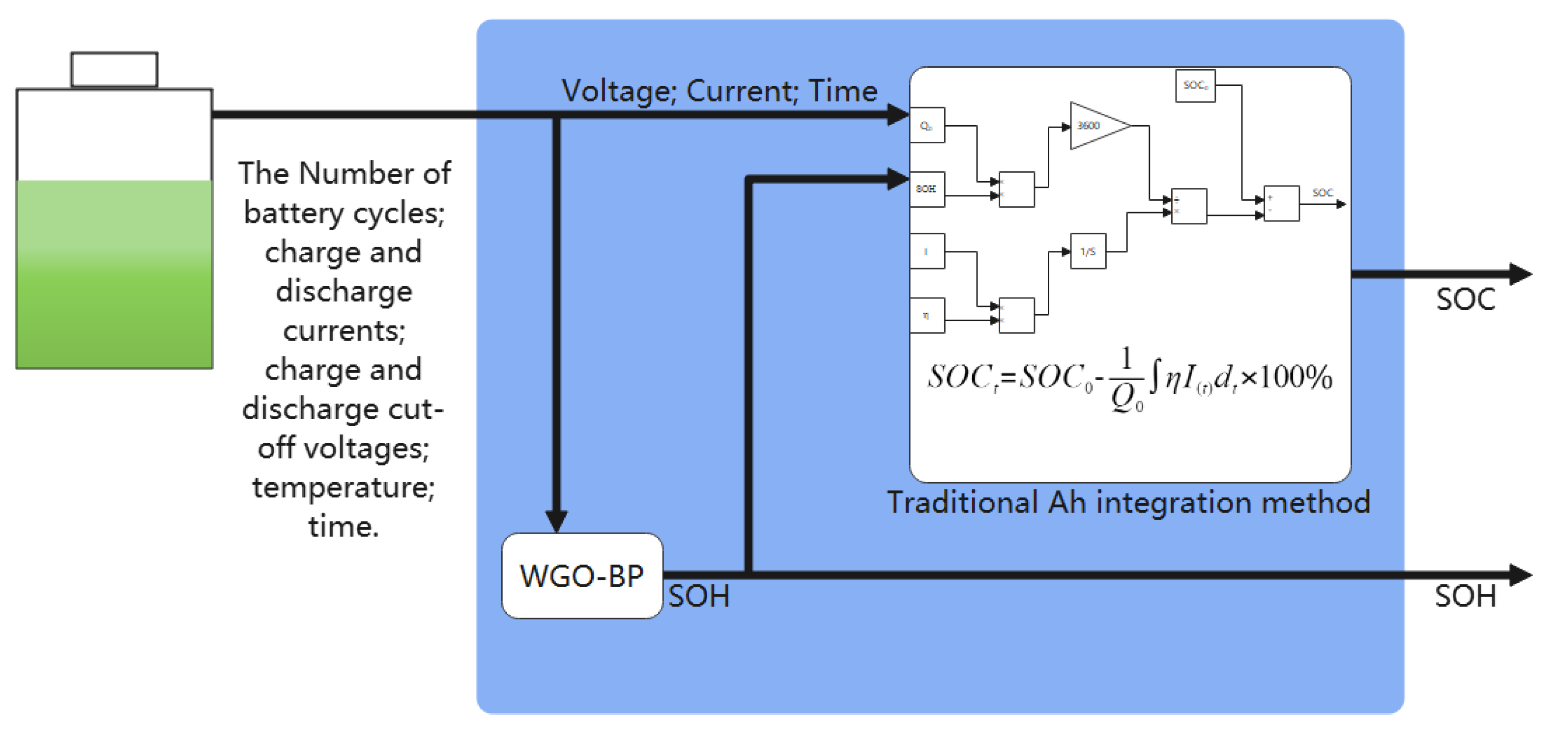
We proposed a joint SOH-SOC estimation model based on neural networks and the traditional Ah integration method.

1.2. Contribution

(1)

We proposed a joint SOH-SOC estimation model based on neural networks and the Ah integration method to optimize the traditional Ah integration method and improve the accuracy of SOC estimation.

(2)

We used the ONLY-BP and GWO-BP neural networks to predict the SOH, and analyzed the resultant errors. We chose the more effective GWO-BP neural network for the SOH prediction part of the joint SOH-SOC estimation model.

(3)

A combination of neural networks and traditional SOC estimation methods were used, with a relatively simple model structure and fast computing speed. It avoided the complexity of SOC estimation caused by the combination of multiple neural networks. The more complex the structure, the greater the error probability, the longer the calculation time, and the lower the timeliness of SOC estimation.

(4)

The battery dataset we used in this paper was a hybrid dataset consisting of a mixture of the 1278 battery data samples collected, the NASA battery dataset, and data from the CALCE battery dataset [16]. The experimental results are all smaller than the specified errors, which further verifies the stability of our proposed joint estimation model.

2. SOH Estimation

2.1. Influencing Factors of SOH

Battery aging is a long-term, complex, non-linear process. SOH is affected by the environment in which the battery is used and its conditions and cannot be measured directly. SOH is a percentage indicating the storage capacity of the battery. It is the battery’s actual power ratio to the rated capacity. Currently, there is no uniform definition of SOH, mainly defined through capacity, power, internal resistance, and the number of cycles. We studied SOH from a capacity perspective.

$$\mathrm{SOH}=\frac{C_{now}}{C_{new}}\ast \mathrm{100\%}$$

(1)

where $C_{now}$ is the current battery capacity; $C_{new}$ is the rated capacity of the battery

In this paper, we used the NASA battery dataset to analyze the main factors affecting battery SOH. The batteries used in this dataset were the same as those used in the data collection experiments in this paper. They were general commercial rechargeable 18,650 batteries, so we used the battery data in this dataset to analyze the main factors affecting SOH. The dataset recorded the changes in battery voltage, current, and temperature over time for each cycle and the actual capacity of battery discharge. This paper adhered to the principle of unique variables for analyzing factors affecting SOH, i.e., only one condition changes in each analysis and the remaining conditions remain unchanged; this method could minimize the interference of irrelevant and additional variables.

Table 1. Statistical table of experimental conditions for batteries.

Battery Number	Charge Cut-Off Voltage	Discharge Cut-Off Voltage	Discharge Rate	Ambient Temperature
46	4.2 V	2.2 V	0.5 C	4 °C
54	4.2 V	2.2 V	1 C	4 °C
5	4.2 V	2.7 V	1 C	24 °C
7	4.2 V	2.2 V	1 C	24 °C
18	4.2 V	2.5 V	1 C	24 °C
25	4.2 V	2 V	1 C	24 °C
29	4.2 V	2 V	2 C	43 °C

shows the experimental conditions of the battery used in this paper for the SOH variation analysis.

According to Table 1, we can see that battery No. 7 and battery No. 54 only differed in the temperature of usage, as shown in Figure 1a. The SOH of battery No. 54 was generally smaller than the SOH of battery No. 7, with a more dramatic change trend and a shorter service life. Because of the low temperature, the chemical activity of battery No. 54 was reduced, resulting in reduced power release. Except for temperature, all test conditions were the same for battery No. 25 and battery No. 29. Battery No. 29 was tested at 43 °C. The effect of high temperatures on battery performance was two-fold. On the one hand, the high temperature accelerated the internal chemical reactions of the battery and improved its efficiency and performance. On the other hand, high temperatures could also accelerate some irreversible chemical reactions inside the battery, reducing the battery’s active material and causing accelerated battery aging. The change in SOH of the battery caused by the above high temperature is shown in Figure 1b. The SOH of battery No. 29 was close to that of battery No. 25 within a certain number of cycles of usage, but as the number of cycles increased, the SOH decreased faster, i.e., the high temperature accelerated the battery’s aging. According to the SOH change rule of the battery in Figure 1, when the battery worked in a suitable temperature range, the battery SOH would decrease slowly, and the service life of the battery would increase; when the temperature exceeded the limit, this would lead to an accelerated decrease in SOH.

As determined from Table 1, the discharge multiplier of battery 46 and battery 54 was 1 C and 0.5 C, respectively. As shown in Figure 2, the SOH of battery 54 was lower than that of battery 46 because of the increased discharge multiplier, the increased heat loss inside the battery, and the reduced discharge.

According to Table 1, the discharge cut-off voltages of battery 5 and battery 18 were 2.7 V and 2.5 V, respectively. In theory, the lower the cut-off voltage, the more power was released and the greater the SOH when the charging voltage was the same. However, as shown in Figure 3, the SOH of battery No. 18 was less than that of battery No. 5, because an improper charge/discharge cut-off voltage had a bad effect on the battery. When the battery was discharged to less than the specified cut-off voltage, the internal resistance of the battery would increase, and the internal heating would become serious, increasing the side reactions significantly and accelerating the battery’s aging.

Combined with the three graphs above, we can see that the battery SOH would decrease as the number of battery cycles increased. Within different cycles, the battery state parameters are not the same, making the battery heating and chemistry not the same, and such differences persist, affecting battery health and aging.

In summary, the parameters such as temperature, charge/discharge multiplier, charge/discharge cut-off voltage, and the number of cycles would have a certain impact on SOH and life. At present, the study of factors affecting battery SOH is still in the qualitative stage, and the degree of influence of these factors on battery aging and the relationship between the various factors is a difficult point of research, as well as a hot spot for research on SOH and battery life. Therefore, we proposed a joint SOH-SOC estimation model that used a GWO-BP neural network to predict the SOH of a battery using the factors affecting SOH as input.

2.2. BP Neural Networks

2.2.1. Principle of BP Neural Network

The BP neural networks are one of the longest-used and most stable neural network models [17]. BP neural networks can store and learn many mappings between input and output data without knowing the mathematical formula for such mappings in advance. This relies heavily on its “propagation of signals forward, transmission of errors backwards“ characteristic. This feature can ensure that when training the BP neural network, its weights (W) and thresholds can be adjusted in real-time according to the errors, improving the prediction accuracy and, thus, achieving the desired results.

Figure 4 shows the individual Network Topology of a BP neural network, designed according to the neurons in the organism. Neurons in a neural network simulate the whole process of neural conflict, with each neuron receiving and processing signal input from other neurons. Multiple cell dendritic terminals receive the external signal and transmit it to the neuron’s interior, where it is located for fusion processing. The neuron summarizes all signals to obtain a total input. The input is compared with the neuronal threshold and then processed by the “activation function” to obtain the final output (this process simulates the cellular activation process). Finally, this output is used as input to subsequent neurons, passing the signal through axons to other neurons or effectors. This process is passed down through the neural network layer by layer.

We enhanced the expressiveness of the model by introducing an activation function. Regardless of the structure of the neural network, in the absence of an activation function, it was simply a linear mapping; thus, the approximation ability of the network was quite limited, and a purely linear mapping could not solve linearly indistinguishable problems. For these reasons, we decided to introduce non-linear functions as excitation functions to enhance the expressive power of the deep neural network.

$V$ and $W$ in Figure 5 are the weights from the input layer to the hidden layer and from the hidden layer to the output layer, respectively.

(1)

Input layer: This is the information input end to reading input data, and there are as many input nodes as there are types of input data.

(2)

Hidden layer: This is the information processing end, divided into one or more layers. The prediction accuracy of a neural network increases with the number of hidden layers, and the structure becomes complex, leading to increased training time and even overfitting. Typically, there is only one hidden layer, and the prediction accuracy is adjusted by changing the number of nodes in the hidden layer.

Figure 5. Basic structure of BP neural network.

Figure 5. Basic structure of BP neural network.

The number of hidden layer nodes significantly impacts the accuracy of a neural network. Still, there is no scientific method to determine the number of hidden layer nodes. If the quantity is too small, the network cannot build complex judgment bounds, cannot train appropriate functions, cannot identify samples that have not appeared before, and is poorly fault-tolerant. If the number of nodes is too big, it will increase the training time, and adaptability will decrease. Therefore, the number of nodes should be minimized to make the network structure more compact, provided that the accuracy requirements are met. At the same time, the number of nodes in the hidden layer must be less than $n-1$ (n is the number of training samples). Otherwise, the built network model has no generalization ability and is useless.

Usually, according to the following formula, the approximate range is determined and the “trial and error method” is used to determine the optimum number of nodes. For some problems, the number of nodes in the hidden layer has less impact on the output.

$$L < n-1$$

(2)

$$L < \sqrt{m+n}+a$$

(3)

$$L < lo{g}_{2}n$$

(4)

where $n$ is the number of nodes in the input layer; l is the number of nodes in the hidden layer; m is the number of nodes in the output layer; a is a constant between 0 and 10.

(3)

Output layer: This is the output of the information, the result we want, and therefore, has the same number of nodes as the number of data we predict.

2.2.2. Building BP Neural network

We used BP neural networks to predict SOH because of their structural simplicity and technical maturity. Figure 6 shows the network structure, including one input layer, one hidden layer, and one output layer. After analysis, the main factors affecting the battery SOH were determined as follows: the number of cycles, discharge start voltage, discharge end voltage, ambient temperature, charge multiplier, and discharge multiplier, which led to the determination that the number of nodes in the input layer was 6. After training the neural network several times, the number of nodes in the hidden layer of the network model was determined to be 18 according to the “trial-and-error” method. As the input data for this network model were SOH, the number of nodes in the output layer was 1.

Figure 7 shows the flow chart of the BP neural network we used, and the specific flow of this model is as follows:

Step 1. Read the data. The training set and prediction set were determined for neural network training. The training set data were normalized; the purpose of normalization was to normalize the samples’ statistical distribution, avoiding the network’s inability to converge due to the presence of odd sample data and speeding up the learning speed of the network.

Step 2. Build the network structure and set the parameters. The main parameters were the number of training sessions, the learning rate, and the minimum error of the training target. In addition, the positions of weights and biases (thresholds) between the layers were marked for later algorithm optimization, such as genetic algorithms.

Step 3. Train the neural network. Neural network training was carried out, and adjusted network parameters were according to the error of prediction results to improve the prediction accuracy. When the prediction accuracy reached a preset value, or the number of training sessions reached a maximum, the network training was stopped.

Step 4. Analyze the prediction results of the prediction set. The trained neural network was used to predict the prediction set data. If the accuracy met the requirement, the neural network model was saved and used for the joint simulation model, and vice versa: the neural network was retrained.

We used mean squared error (MSE) as the loss function in the backward propagation of the model. This paper describes the estimation accuracy of the neural network by MAE and RMSE.

$$\mathrm{MSE}=\frac{1}{M}{{\displaystyle \sum _{i=1}^M\left(y_i-{\widehat{y}}_i\right)}}^2$$

(5)

$$\mathrm{MAE}=\frac{1}{n-T}{\displaystyle \sum _{t=T+1}^n‖x_t-{\widehat{x}}_t‖}$$

(6)

$$\mathrm{RMSE}=\sqrt{\frac{1}{n-T}{\displaystyle \sum _{t=T+1}^n{(x_t-{\widehat{x}}_t)}^2}}$$

(7)

2.3. Grey Wolf Optimizer

Grey Wolf Optimizer (GWO) was pioneered by Australian Griffith University academic MirJalili et al. in 2014 [18]. The algorithm is an optimized algorithm for simulating the predation process of the grey wolf, with few parameters and easy implementation. Therefore, we chose it to optimize the BP neural network.

According to the individual strength of each grey wolf, the pack is divided into four strata: $\alpha , \beta , \delta$, and $\omega$, where $\alpha$ is the head wolf, i.e., the optimal solution generated by the optimization algorithm; $\beta$ is the suboptimal solution, obeying only $\alpha$; the third stratum $\delta$ obeys $\alpha$ and $\beta$ and leads $\omega$; all the remaining wolves are $\omega$.

The GWO optimization process consists of three main parts.

Step 1. Social hierarchy stratification (initializing the population). When designing GWO, the hierarchy of the gray wolf population needs to be constructed first. The suitability of each grey wolf is compared, and the three best-adapted grey wolves in the pack are labeled $\alpha , \beta ,$ and $\delta$, with the remaining individuals being labeled $\omega$. The hierarchical differentiation of wolves is not static and will be updated with the results of each iteration.

Step 2. Surround prey (population search). When gray wolves search for prey, they will gradually approach and surround the prey. For the mathematical model of this behavior, see Equations (8) and (9):

$$\overrightarrow{\mathrm{D}}=\left|\overrightarrow{\mathrm{C}}\ast \overrightarrow{X_p}(t)-\overrightarrow{X}(t)\right|$$

(8)

$$\overrightarrow{X}(t+1)=\overrightarrow{X_p}(t)-\overrightarrow{A}\ast \overrightarrow{D}$$

(9)

where $\overrightarrow{D}$ is the distance between the prey and the grey wolf; t is the number of iterations; $\overrightarrow{C}$ and $\overrightarrow{A}$ are the coefficient vectors; $\overrightarrow{X}$ and ${\overrightarrow{X}}_p$ are the grey wolf position vector and the prey position vector, respectively.

For the calculation equation of vectors $\overrightarrow{C}$ and $\overrightarrow{A}$, see Equation (10) and Equation (11):

$$\overrightarrow{A}=2\ast \overrightarrow{a}\ast \overrightarrow{r_1}-\overrightarrow{a}$$

(10)

$$\overrightarrow{C}=2\ast \overrightarrow{r_2}$$

(11)

where $\overrightarrow{r_1}$ and $\overrightarrow{r_2}$ are random numbers in the range [(0,1); $\overrightarrow{a}$ is the convergence factor, which takes values in the range (0,2) and decreases linearly with the number of iterations of the algorithm. Corresponding to Equation (10), $\left|\overrightarrow{A}\right|\ge 1$ means that performing a global search and vice versa means that the grey wolf conducts a local examination.

Step 3. Hunting (updating population location). After determining the location of prey, grey wolves rely on information from $\alpha , \beta ,$ and $\delta$ to guide them to surround prey. In practical applications, the spatial characteristics of many problems are unknown, and the grey wolf cannot determine its prey’s exact location. As in Figure 8, the change in position during a grey wolf hunt is mimicked, assuming that $\alpha , \beta ,$ and $\delta$ can identify the location of potential prey. The remaining grey wolf positions are then updated based on the position information of the first three optimal solutions, $\alpha , \beta ,$ and $\delta$, during each iteration.

The mathematical expression for the change in the position of individual grey wolves throughout the update is as follows.

$$\left\{\begin{array}{c}\overrightarrow{D_{\alpha }}=\left|\overrightarrow{C_1}\ast \overrightarrow{X_{\alpha }}-\overrightarrow{X}\right|\\ \overrightarrow{D_{\beta }}=\left|\overrightarrow{C_2}\ast \overrightarrow{X_{\beta }}-\overrightarrow{X}\right|\\ \overrightarrow{D_{\delta }}=\left|\overrightarrow{C_3}\ast \overrightarrow{X_{\delta }}-\overrightarrow{X}\right|\end{array}\right.$$

(12)

$$\left\{\begin{array}{c}\overrightarrow{X_1}=\overrightarrow{X_{\alpha }}-A_1\ast \overrightarrow{D_{\alpha }}\\ \overrightarrow{X_2}=\overrightarrow{X_{\beta }}-A_2\ast \overrightarrow{D_{\beta }}\\ \overrightarrow{X_3}=\overrightarrow{X_{\delta }}-A_3\ast \overrightarrow{D_{\delta }}\end{array}\right.$$

(13)

$$\overrightarrow{X_{t+1}}=\frac{\overrightarrow{X_1}+\overrightarrow{X_2}+\overrightarrow{X_3}}{3}$$

(14)

where $\overrightarrow{D_{\alpha }}, \overrightarrow{D_{\beta }}$, and $\overrightarrow{D_{\delta }}$ represent the distances between $\alpha ,\beta ,$ and $\delta$ in terms of other individuals, respectively; $\overrightarrow{X_{\alpha }}, \overrightarrow{X_{\beta }}, \mathrm{and}\overrightarrow{X_{\delta }}$ represent $\alpha ,\beta ,$ and $\delta$ positions, respectively; $\overrightarrow{C_1}, \overrightarrow{C_2}, \mathrm{and} \overrightarrow{C_3}$ are random vectors; $\overrightarrow{X}$ indicates the current location of the individual grey wolf.

Equation (13) defines the step size and direction of movement of a single $\omega$ wolf, toward $\alpha ,\beta ,$ and $\delta$ wolves; Equation (14) determines the final position of this $\omega$ wolf movement.

Figure 9 shows a flow chart of the Grey Wolf optimization algorithm:

2.4. Comparison of Errors

The ONLY-BP and GWO-BP neural networks were used to predict the battery SOH, and the results were compared to select the neural network with less error for use in the joint SOH-SOC estimation model. Both neural networks were built based on MATLAB and the learning efficiency of ONLY-BP was set to 0.001, the maximum number of cycles was 1000, and the minimum training error was 0.001. The GWO-BP neural network was built based on the ONLY-BP neural network and was an optimization method for ONLY-BP. We only needed to design the parameters of GWO-BP with a population size of 20, a maximum number of iterations of 40, and a threshold upper and lower bound of ±2. We used the 1278 sets of battery data collected during the experimental phase of this paper as the training set. We used the 168 sets for battery 5 from the NASA battery dataset as the prediction set.

Figure 10 shows the error variation curves of the two neural networks. Ten random estimations were performed for the two neural networks, respectively, and the MAE, MSE, and RMSE were taken to indicate the errors in the estimation results. As can be seen from Figure 10, the GWO-BP neural network error was much smaller and varied very smoothly. Therefore, this paper chose the GWO-BP neural network for the SOH prediction part of the joint SOH-SOC model.

3. SOC Estimation

3.1. Ah Integration Method

SOC is defined as the ratio of the remaining charge after battery use to the charge at the start of discharge, usually in the form of a percentage, according to the following formula [19].

$${\mathrm{SOC}}_t=\frac{Q_t}{Q_0}\times 100\%$$

(15)

where $Q_t$ is the remaining battery charge; $Q_0$ is the rated capacity of the battery; SOC ranges from 0 to 100%; 100% means the battery is fully charged and 0 means the battery is fully discharged.

The Ah integration method determines the amount of electricity released from the battery by integrating the current over time and calculates the battery SOC [20], as shown in Equation (16).

$$SO{C}_t=SO{C}_0-\frac{Q_i}{Q_0}\times 100\%=SO{C}_0-\frac{1}{Q_0}{\displaystyle \int \eta I_{(t)}}dt\times 100\%$$

(16)

where $SO{C}_t$ is the remaining battery charge at time $t$; $SO{C}_0$ is the initial battery charge; $Q_i$ is the amount of electricity released from the battery at the moment $0-t$; $Q_0$ is the nominal battery charge and is a constant; $\eta$ is the charging and discharging efficiency, usually taken as 1; $I_{\left(t\right)}$ is the cell current, in the positive direction of discharge.

Although the Ah integration method can improve the accuracy of $Q_i$ by integration, the effect of SOH on battery capacity is not considered in the calculation process, increasing errors in SOC estimation. To address this problem, this paper proposed a joint SOH-SOC estimation model based on neural networks and the Ah integration method, which fully considers the influence of SOH on SOC and improves the accuracy of SOC estimation.

3.2. Joint SOH-SOC Estimation Model

We proposed a joint SOH-SOC estimation model based on GWO-BP to achieve the joint estimation of SOH and SOC, and its structure is shown in Figure 11. The part of the Ah integration method was built through MATLAB/Simulink, as shown in Figure 12. $Q_0$ was the battery’s rated capacity (constant), and the SOH predicted by the GWO-BP neural network was introduced to correct $Q_0$ to make it close to the actual capacity of the current battery and improve the accuracy of the SOC calculation.

4. Testing and Analysis

A total of 1278 sets of experimental data from six 18650 batteries were collected. In addition, 168 datasets for battery 5 in the NASA battery dataset and 100 sets of data from the CALCE battery dataset were introduced in the experimental phase of this paper, in order to verify the accuracy and stability of the joint SOH-SOC estimation model proposed in this paper.

A total of two sets of comparative trials were conducted in this paper:

(1)

A comparative analysis of the accuracy of the ONLY-BP and GWO-BP neural networks for predicting battery SOH was conducted to select one of the estimation methods with higher accuracy for the joint SOH-SOC estimation model.

(2)

The accuracy of predicting battery SOC was compared between the conventional Ah integration method and the joint SOH-SOC estimation model.

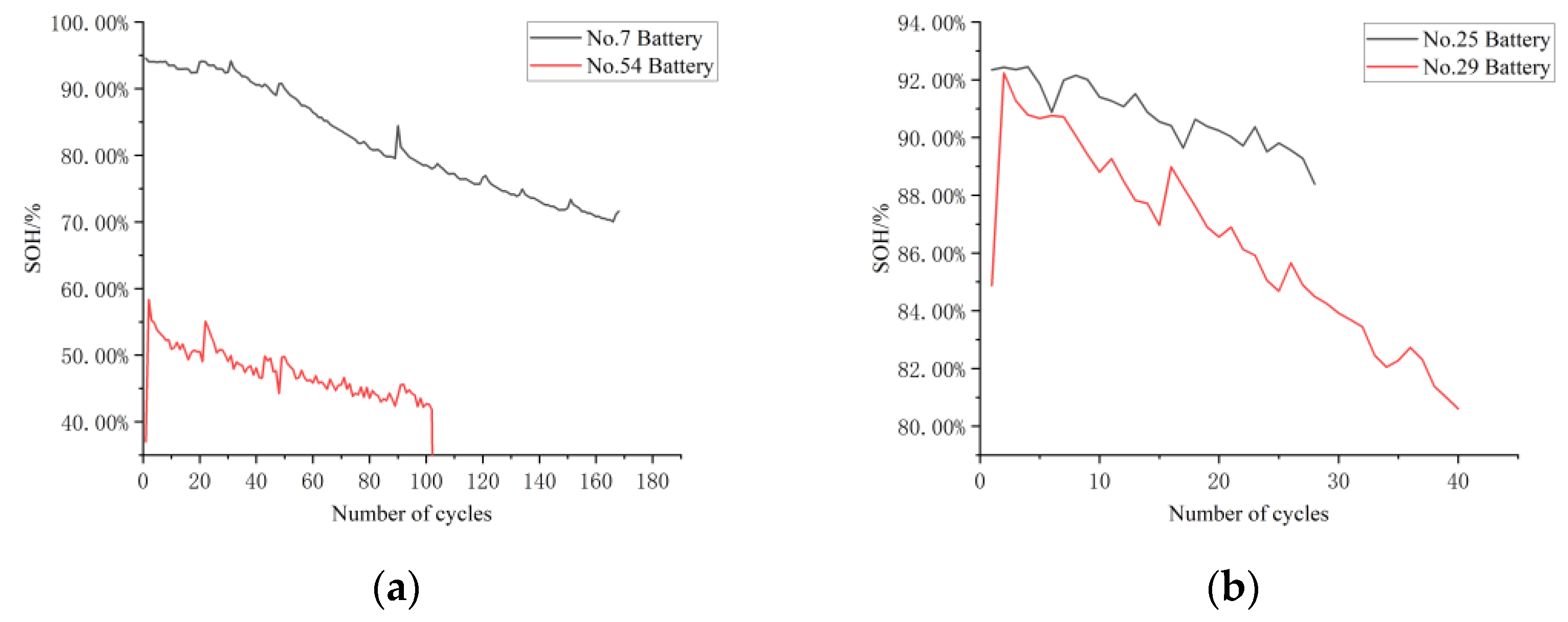
4.1. Acquisition of Test Data

The test battery selected for this paper was a general commercial rechargeable 18650 battery. The main parameters of this type of battery are shown in

Table 2. Main parameters of 18650 batteries.

Capacity/mAh	2000	Charge cut-off voltage/V	4.2
Discharge cut-off voltage/V	2.75	Nominal voltage/V	3.7
Anode materials	Ternary materials	Negative electrode materials	Amorphous carbon

.

In the test process described in this paper, the main test instrument was a four-channel lithium battery capacity detector, which had four independent data acquisition channels, and could simultaneously collect data from four batteries under different experimental conditions without mutual interference. The device could also display real-time parameters such as battery voltage, current capacity, and temperature.

This test was conducted at room temperature to make the test conditions more realistic. Using the test equipment, the battery’s charging/discharge cut-off voltage was set to 4.2 V and 2.75 V, the discharge rate was set to 0.25 C, the charge rate was set to 0.5 C, and the battery was emptied and recharged, which was a charging cycle. Based on the previous analysis of the battery SOH variation, a total of 6 parameters, such as the number of battery cycles, charge/discharge cut-off voltage, charge/discharge multiplier, and the ambient temperature of the battery, were collected in the test, with a total of 1278 sets of data collected.

4.2. Verification of Test

The joint SOH-SOC estimation model proposed in this paper and the conventional model of the Ah integration method were established by MATLAB, and the same battery SOC was estimated at the same time to compare the estimation errors.

This was implemented as follows:

Step 1. Build the algorithm models. Two models of SOC estimation methods were built in MATLAB. After comparing the accuracy of the GWO-BP and ONLY-BP neural networks in the early stage, this experiment chose the GWO-BP neural network to complete the SOH estimation part of the joint SOH-SOC estimation model.

Step 2. Training neural networks. The battery data, imported into the neural network, were divided into training and prediction sets. The number of battery cycles, charge and discharge cut-off voltages, charge and discharge multipliers, and the operating ambient temperature of the battery were used as input data for the GWO-BP, and the battery SOH was used as output data. The neural network parameters were updated based on the prediction results to improve the prediction accuracy.

Step 3. Complete the comparison experiment. The data from the same battery were brought into the two SOC estimation models for SOC estimation, and error analysis was performed to verify the accuracy of the joint SOH-SOC estimation model proposed in this paper.

4.3. Analysis of Experimental Results

In order to verify the accuracy of the joint SOH-SOC estimation model proposed in this paper, battery 5 in the NASA battery dataset was used as the test object in this paper. The two SOC estimation models were used separately to complete the SOC estimation, and the errors of the estimated results were analyzed.

The error of the GWO-BP neural model for the SOH estimation of battery No. 5 was MAE = 0.025864, MSE = 0.00119, and RMSE = 0.034448.

The cell-out data for each use cycle of battery No. 5 was taken as the two SOC estimation models to complete the SOC estimation. In order to further verify the accuracy of the SOH-SOC joint estimation model, we also used a “SOC estimation method based on LSTM neural network” in this comparison stage to estimate the SOC of the No. 5 battery. Figure 13 illustrates the error between the estimated results of the three SOC estimation models and the actual SOC values.

According to the national standard, QC/T897-2011, “Technical conditions for a battery management system for electric vehicles,” the system is qualified if the SOC estimation accuracy reaches 10%. As shown in Figure 13, the error in the results by the traditional Ah integration method increased as the number of battery cycles increased until the specified requirements were exceeded. The traditional Ah integration method ignored the effect of SOH in SOC estimation and used the battery’s rated capacity in the calculation process. As the battery ages with increased use, the SOH tends to decline, resulting in reduced battery capacity and increased errors until it is outside the specified range. The SOC estimation method based on LSTM neural network has a minor error in SOC estimation, but it is still higher than the SOH-SOC joint estimation model proposed in this paper. The joint SOH-SOC estimation model proposed in this paper could stabilize the estimation result error within 5% within any number of cycles, which met the national standard. It reduced the error of the traditional Ah integration method and improved SOC estimation accuracy.

We separately put the data of the charge and discharge process in the fifth cycle of the No. 5 battery in the NASA battery dataset into the two SOC estimation methods for SOC estimation. The test results are shown in Figure 14.

As shown in Figure 14, the SOC value predicted by the joint SOH-SOC estimation model was much closer to the actual SOC value, whether the battery was in the charging or discharging process, further validating the accuracy of the joint SOH-SOC estimation model.

The accuracy of the joint SOH-SOC estimation model can be well demonstrated in Figure 13 and Figure 14 above. Moreover, to further illustrate the generality of the joint SOH-SOC estimation model, we took 100 battery datasets from the CALCE battery dataset as the subject of our study. We estimated them separately using the two SOC estimation methods, with the resulting errors shown in Figure 15.

As shown in Figure 15, the SOC error estimated by the joint SOH-SOC estimation model could be stable within 5%. The error would not exceed the specified limit even if the battery data fluctuated. In contrast, the traditional Ah estimation method’s estimation error was not stable, fluctuated drastically, and could even approach 25%.

5. Summary

After analyzing the shortcomings of the traditional Ah integration method, we proposed a joint SOH-SOC estimation model based on neural networks. The GWO-BP neural network was used for battery SOH prediction, and the prediction was introduced into the Ah integration method to correct the battery capacity and improve the accuracy of SOC estimation.

We used the joint SOH-SOC estimation model and the traditional Ah integral method model to estimate SOC for the battery data in the CALCE battery dataset and the No. 5 battery in the NASA battery dataset, respectively. After comparing the errors in the estimation results, we found that the errors estimated by the traditional Ah integration method would increase with the number of cycles until the national safety standards were exceeded. However, the estimation error of the joint SOH-SOC estimation model proposed in this paper was stable within 5%, much less than the national regulation of 10%, and the SOC estimation accuracy was higher. Moreover, the addition of SOH prediction gave the driver a more diverse view of the battery’s status and a more three-dimensional battery status. In our experiments, we used a hybrid dataset of the battery data collected in this paper with the NASA and CALCE battery datasets. The accuracy of the final prediction results met the requirements and verified the stability of the joint SOH-SOC estimation model.

References

1. Chemali, E.; Preindl, M.; Malysz, P.; Emadi, A. Electrochemical and Electrostatic Energy Storage and Management Systems for Electric Drive Vehicles: State-of-the-Art Review and Future Trends. IEEE. Emerg. Sel. Top. Power Electron. 2016, 4, 1117–1134. [Google Scholar] [CrossRef]
2. Zheng, Y.; Lu, Y.; Gao, W.; Han, X.; Feng, X.; Ouyang, M. Micro-Short-Circuit Cell Fault Identification Method for Lithium-Ion Battery Packs Based on Mutual Information. IEEE Trans. Ind. Electron. 2021, 68, 4373–4381. [Google Scholar] [CrossRef]
3. Hannan, M.A.; Lipu, M.H.; Hussain, A.; Mohamed, A. A review of lithium-ion battery state of charge estimation and management system in electric vehicle applications: Challenges and recommendations. Renew. Sustain. Energy Rev. 2017, 78, 834–854. [Google Scholar] [CrossRef]
4. Huang, S.C.; Tseng, K.H.; Liang, J.W.; Chang, C.L.; Pecht, M.G. An online SOC and SOH estimation model for lithium-ion batteries. Energies 2017, 10, 512. [Google Scholar] [CrossRef]
5. Yang, Q.; Ma, K.; Xu, L.; Song, L.; Li, X.; Li, Y. A Joint Estimation Method Based on Kalman Filter of Battery State of Charge and State of Health. Coatings 2022, 12, 1047. [Google Scholar] [CrossRef]
6. Ahmed, M.S.; Balasingam, B. A scaling approach for improved open circuit voltage modeling in Li-ion batteries. In Proceedings of the 2019 IEEE Electrical Power and Energy Conference (EPEC), Montréal, QC, Canada, 16–18 October 2019; pp. 1–6. [Google Scholar]
7. Wei, Z.; Zhao, D.; He, H.; Cao, W.; Dong, G. A noise-tolerant model parameterization method for lithium-ion battery management system. Appl. Energy 2020, 268, 114932. [Google Scholar] [CrossRef]
8. Jin, G.; Li, L.; Xu, Y.; Hu, M.; Fu, C.; Qin, D. Comparison of SOC Estimation between the Integer-Order Model and Fractional-Order Model Under Different Operating Conditions. Energies 2020, 13, 1785. [Google Scholar] [CrossRef] [Green Version]
9. Hou, E.; Xu, Y.; Qiao, X.; Liu, G.; Wang, Z. State of power estimation of echelon-use battery based on adaptive dual extended Kalman filter. Energies 2021, 14, 5579. [Google Scholar] [CrossRef]
10. Qiao, X.; Wang, Z.; Hou, E.; Liu, G.; Cai, Y. Online Estimation of Open Circuit Voltage Based on Extended Kalman Filter with Self-Evaluation Criterion. Energies 2022, 15, 4373.n. [Google Scholar] [CrossRef]
11. Lai, X.; Yuan, M.; Tang, X.; Yao, Y.; Weng, J.; Gao, F.; Ma, W.; Zheng, Y. Co-Estimation of State-of-Charge and State-of-Health for Lithium-Ion Batteries Considering Temperature and Ageing. Energies 2022, 15, 7416. [Google Scholar] [CrossRef]
12. Tian, H.; Chen, J. Deep Learning with Spatial Attention-Based CONV-LSTM for SOC Estimation of Lithium-Ion Batteries. Processes 2022, 10, 2185. [Google Scholar] [CrossRef]
13. Shahriar, S.M.; Bhuiyan, E.A.; Nahiduzzaman, M.; Ahsan, M.; Haider, J. State of Charge Estimation for Electric Vehicle Battery Management Systems Using the Hybrid Recurrent Learning Approach with Explainable Artificial Intelligence. Energies 2022, 15, 8003. [Google Scholar] [CrossRef]
14. Yang, B.; Wang, Y.; Zhan, Y. Lithium Battery State-of-Charge Estimation Based on a Bayesian Optimization Bidirectional Long Short-Term Memory Neural Network. Energies 2022, 15, 4670. [Google Scholar] [CrossRef]
15. Meng, J.; Boukhnifer, M.; Diallo, D. Lithium-Ion Battery Monitoring and Observability Analysis with Extended Equivalent Circuit Model. In Proceedings of the 2020 28th Mediterranean Conference on Control and Automation (MED), Saint-Raphaël, France, 5–18 September 2020; pp. 764–769. [Google Scholar]
16. Dos Reis, G.; Strange, C.; Yadav, M.; Li, S. Lithium-ion battery data and where to find it. Energy AI 2021, 5, 100081. [Google Scholar] [CrossRef]
17. Zheng, Y.; Lv, X.; Qian, L.; Liu, X. An Optimal BP Neural Network Track Prediction Method Based on a GA–ACO Hybrid Algorithm. J. Mar. Sci. Eng. 2022, 10, 1399. [Google Scholar] [CrossRef]
18. Seyedali, M.; Seyed, M.M.; Andrew, L. Grey Wolf Optimizer. Adv. Eng. Softw. 2014, 69, 46–61. [Google Scholar]
19. Jafari, S.; Shahbazi, Z.; Byun, Y.-C.; Lee, S.-J. Lithium-Ion Battery Estimation in Online Framework Using Extreme Gradient Boosting Machine Learning Approach. Mathematics 2022, 10, 888. [Google Scholar] [CrossRef]
20. Ding, Z.T.; Deng, T.; Li, Z.F.; Yin, Y.L. Research on SOC estimation method for lithium-ion batteries based on Ah integral and traceless Kalman filter. China Mech. Eng. 2020, 31, 1823–1830. [Google Scholar]
Figure 1. Change curve of SOH at different temperatures. (a) SOH change curve for battery 7 and battery 54. (b) SOH change curve for battery 25 and battery 29.
Energies 16 00132 g001
Figure 2. Change curve of SOH at different discharge rates.
Energies 16 00132 g002
Figure 3. Change curve of SOH at different discharge cut-off voltages.
Energies 16 00132 g003
Figure 4. Topological structure of neurons.
Energies 16 00132 g004
Figure 6. BP neural network structure.
Energies 16 00132 g006
Figure 7. Flow chart of neural network training.
Energies 16 00132 g007
Figure 8. Schematic diagram of wolf location update.
Energies 16 00132 g008
Figure 9. Flow chart of the Grey Wolf optimization algorithm.
Energies 16 00132 g009
Figure 10. Error analysis of random 10-time neural network prediction.
Energies 16 00132 g010
Figure 11. Schematic diagram of the SOH-SOC estimation model.
Energies 16 00132 g011
Figure 12. Simulink structure of the time-integration method.
Energies 16 00132 g012
Figure 13. SOC estimation error for No. 5 battery.
Energies 16 00132 g013
Figure 14. SOC change curve for the 5th use cycle of the No. 5 battery. (a) Charging process SOC change curve. (b) Discharging process SOC change curve.
Energies 16 00132 g014
Figure 15. CALCE battery data error curve.
Energies 16 00132 g015