Risk Assessment of User Aggregators in Demand Bidding Markets

Abstract

This paper mainly discusses the demand bidding and risk management of user aggregators by considering profit and risk. The covariance matrix of demand price was used to analyze the risk model under an uncertain demand price. By considering revenue and cost, the demand bidding strategy of user aggregators was derived to obtain the maximum profit. By using a risk-tolerance parameter β, a new demand bidding model for the user aggregators that takes both risk and profit into consideration was formulated. We simulated the risk posed by fluctuating demand prices for user aggregators using this model. Finally, this paper proposes Feasible Particle Swarm Optimization (FPSO) to solve the demand bidding model of user aggregators. Through the dynamic adjustment of control factor parameters in the FPSO, we changed the behavioral characteristics of various types of particles, improved the search efficiency and stability of particles in high-dimensional space, and sought the optimal solution for the system as a whole. This paper provides a parameter adjustment mechanism, improves the capability of algorithm implementation, and increases the probability of finding the optimal solution. The simulation results suggest that a tradeoff between profit and risk needs to be considered in the search process. By doing so, enterprises’ abilities in terms of operation and management control can be enhanced, and effective demand management can be achieved.

1. Introduction

In recent years, the overall investment environment in Taiwan has been booming, and electricity consumption has reached a record high every year. The gap between peak load and off-peak load continues to increase every year. The ratio between the summer peak load during the day and the off-peak load at night is about 1:0.61, and the maximum summer load is about 1.4 times that of the maximum non-summer load [1]. This shows that there is still a great difference in load between different seasons and between the peak load and off-peak load of the power system. In order to reflect the power supply cost difference between the peak and off-peak power consumption in summer and non-summer months, the Taiwan Power Company (TPC) implements an electricity price system based on seasons and time to control the peak load and improve the power supply [2]. Electricity users can cooperate with the power company to implement load management and reduce power consumption in peak periods without affecting their electricity demand or normal operation. Therefore, it could improve their willingness to participate the implementation performance of this system. In addition, electricity users could also obtain some revenue due to favorable feedback and compensation from the power company. All of these could be more beneficial through the utilization rate of power equipment and enhancing the quality of electricity utilization. If operators could effectively implement these to reduce the problem of excessive peak load through shifting the electricity consumption during peak periods to off-peak periods, achieve power balance, and reduce the construction demand of new power plants, it would effectively improve the electricity supply and ensure that power companies and enterprise users achieve a mutually beneficial situation. Therefore, for load management, the research and development of a demand management strategy is one of the most important policy directions [3].

The demand response (DR) strategy is one of the measures taken by power companies to reduce electricity consumption, and this strategy could provide incentives to reduce electric charges. During periods when the power supply is low or the cost is high, electricity users could cooperate to reduce the agreed electricity load and consumption, which could have a very significant effect on system load reduction in peak periods. This strategy could reduce the burden of electricity charges on users for electricity consumption, and it has gradually started to attract the attention of enterprise users. In the demand response mechanism, such as the planned electricity reduction measures or demand bidding strategy [4], the electricity load and consumption reduced by electricity users could obtain high benefits through participating in the demand bidding strategy. Under the framework of a demand bidding strategy, power companies could provide electricity price discounts or other market incentive mechanisms, and the aggregator representative of electricity users could reduce the electricity load and consumption during periods of low peak electricity supply for many users according to the needs of the power company by means of demand bidding. The concept of Virtual Peaking Capacity (VPC) [5] could generate electric resources not only from the central power system but also from the distributed power generation system at the power load end under the “real-time” and “two-way” approaches. Therefore, in comparison with traditional systems, the electricity supply and demand are multi-variant and more flexible. In addition, through the implementation of energy saving plans, it could reduce the electricity consumption demand of power users.

In recent years, demand management strategies for the electricity market have mainly focused on the effects of various operation strategies on profit. Some studies have effectively demonstrated how to solve these problems in the electricity market. Reference [6] incorporated price-based demand response to perform the optimal dispatch schedule in the day-ahead electricity market. A new demand bidding strategy for the smart building aggregator was proposed to perform demand response in the electricity market [7]. References [8,9] proposed a bi-level model for the demand bidding strategy of load agents with incentive-based demand response in day-ahead electricity markets. Based on game theory, [10] proposed an optimal bidding strategy for demand response in the electricity market. A dynamic demand bidding strategy for an aggregator was proposed to participate in the frequency regulation market [11]. A demand response model between the integrated energy production base, load aggregator, and user is established, which is solved by a mixed-integer quadratic programming–multi-verse optimizer distributed algorithm [12]. Reference [13] proposed a novel approach for incorporating incentive-based and price-based demand response programs in long-term generational investment planning. Reference [14] established an energy management platform by integrating distributed power and energy storage to perform the demand bidding strategy. The common disadvantage of the methods described is the lack of guarantee that the profit may be at risk due to the uncertainties of the electricity price. While some risk was expected in the formation and operation of demand response, addressing uncertainties would be a key issue in studying this topic.

Risk management has become an essential condition for the sustainable operation of the power generation industry [15,16]. The demand bidding strategy of user aggregators is particularly important for the degree of risk of profit [17]. The risk assessment would analyze the possible risks faced by each system during power dispatching and pricing and discuss the maximum profit of demand bidding for user aggregators and the corresponding risk after considering the risk limit. However, in the demand bidding strategy, representatives of users could integrate many different electricity users and sign contracts with them under the participation conditions of demand response [18,19,20]. This study analyzed the demand bidding of user aggregators and considered the maximum profit after taking profit and risk into consideration. The demand price variability is used to generate demand price variation to establish a covariance matrix of demand price [21], which is used to analyze the risk level of demand bidding for user aggregators. The effect of risk is explicitly introduced in the bidding strategy problem, considering the variance in demand prices. The tradeoff model between profit and risk is properly addressed within a given risk tolerance. Finally, this paper proposed a Feasible Particle Swarm Optimization (FPSO) to solve the demand bidding model of user aggregators. In the FPSO procedure, the dynamic control parameters are embedded in the particle swarm of the FPSO to improve the behavior patterns of each particle swarm and increase its search efficiency and accuracy in high dimensions. Different modifications in the moving patterns of FPSO are proposed to search the feasible space more effectively. The results can help decision-makers optimize the tradeoffs between maximum profit and minimum risk. In addition to helping decision-makers improve system operation safety, energy efficiency, and risk management, this study can also explore the economic benefits of different decisions in the architecture and planning of energy management systems.

2. Risk Model for Demand Bidding

In Taiwan, the model of planning electricity consumption reduction allows users to evaluate their characteristics for obtaining their maximum profit. Three models were developed by the Taiwan Power Company, which included an 8 day monthly reduction model, a 6 h daily reduction model, and a 2 h daily reduction model [22]. The implementation period was from June 1 to September 30 each year [22]. In the 8 day monthly reduction model, the suppression of electricity consumption occurs from Monday to Friday every month, and the suppression of electricity consumption time is 10 a.m. to 5 p.m. In the 6 h daily reduction model, the suppression of electricity consumption occurs from Monday to Friday every month, and the suppression of electricity consumption times are 10–12 a.m. and 1–5 p.m. In the 2 h daily reduction model, the suppression of electricity consumption occurs from Monday to Friday every month, and the suppression of electricity consumption time is 1–3 p.m. This paper adopted the 6 h daily reduction model to analyze the risk of demand bidding by user aggregators. The suppression of electricity consumption occurs from 10 a.m. to 12 p.m. and from 1 p.m. to 5 p.m. daily during non-holidays. This study utilized the uncertain demand price in the electricity market to generate the demand price variation and establish the covariance matrix of the demand price to analyze the risk of demand bidding by user aggregators. The procedure is described as follows:

• In the day-ahead demand-bidding market, the revenue of the user aggregators is defined as follows:

  $$Revnue={\displaystyle \sum _{t=1}^T{\lambda }_t{p}_t}$$

  (1)

  in the day-ahead demand bidding market, the average revenue of the user aggregator can be obtained by adding the power demand that can be sold at the estimated power expectation for each period (the total demand amount of user aggregators). The expected revenue operator in total periods can be changed as follows:

  $$R^{\exp }={\displaystyle \sum _{t=1}^T{E}_{{\lambda }_t}\left\{{\lambda }_t\right\}{p}_t}$$

  (2)

  where $p_t$ is the power demand (MW) bid by the user aggregator during the period $t$, and $R^{est}$ is the expected total revenue of the user aggregator. ${\lambda }_t$ is the demand price of the user aggregator during the period $t$. $T$ is the total period of demand bidding (the total peak period was 6 h which included from 10 a.m. to 12 p.m. and from 1 p.m. to 5 p.m. $E_{{\lambda }_T}$ is the expected value operator of the random variable ${\lambda }_T$;
• During the 6 h of the peak period, the profits of each period affect each other. The total variation value of revenue during the peak period of 6 h is calculated as follows:

  $$Va{r}_{{\lambda }_1,\cdots ,{\lambda }_T}\left\{{\displaystyle \sum _{t=1}^T{\lambda }_t{p}_t}\right\}={\displaystyle \sum _{t=1}^T{\displaystyle \sum _{j=1}^T{p}_i{V}_{ij}{p}_j}}$$

  (3)
  $Va{r}_{{\lambda }_1},\cdots ,Va{r}_{{\lambda }_T}$ is the variance operator of the random variable.
  $V=(V_{ij})$ is the $T\times T$ covariance matrix of the demand price ${\lambda }_1,\cdots ,{\lambda }_T$.
  $p_i$ and $p_j$ are the power demand (MW) bid by the user aggregators, and they are converted into rows and columns. Because the demand price is the only random variable, the variation of total profit can be expressed by taking the demand price as the covariance matrix. The covariance matrix of the $d$ day is:

  $$V=E_{{\lambda }_1,\cdots ,{\lambda }_T}{\left\{\hspace{0.17em}\left({\wedge }_d^{\mathrm{true}}-{\wedge }_d^{\mathrm{est}}\right)\hspace{0.17em}{\left({\wedge }_d^{\mathrm{true}}-{\wedge }_d^{\mathrm{est}}\right)}^{\mathrm{T}}\right\}}^{}$$

  (4)

  $${\mathrm{\Lambda }}_d={\left[{\lambda }_1,\cdots ,{\lambda }_T\right]}^{\mathrm{T}};$$
• If the bidding history data of the demand trading market are collected up to $d-1$ day, the covariance matrix formula of $d$ day can be expressed by the actual and predicted values as follows:

  $$V^{\mathrm{est}}=\frac{1}{D}{\displaystyle \sum _{i=1}^D({\mathrm{\Lambda }}_i^{\mathrm{true}}-{\mathrm{\Lambda }}_i^{\mathrm{est}})\hspace{0.17em}{({\mathrm{\Lambda }}_i^{\mathrm{true}}-{\mathrm{\Lambda }}_i^{\mathrm{est}})}^T}$$

  (5)

  where ture represents the superscript of the actual value, and $D$ is the total number of days that is the greatest and contains $d-1$ day. When Equation (5) is directly used, due to the nature of the price characteristics of the demand trading market, they may have multiple seasonal characteristics and high variability, as well as unusual purchase prices affected by high load;
• In order to obtain an accurate prediction, it could be modified with the exponentially weighted moving average equation [23]:

  $$V^{\mathrm{est}}=(1-\alpha ){\displaystyle \sum _{i=1}^D{\alpha }^{i-1}({\mathrm{\Lambda }}_{D-i+1}^{\mathrm{true}}-{\mathrm{\Lambda }}_{D-i+1}^{\mathrm{est}})\hspace{0.17em}{({\mathrm{\Lambda }}_{D-i+1}^{\mathrm{true}}-{\mathrm{\Lambda }}_{D-i+1}^{\mathrm{est}})}^T}$$

  (6)

  where $\mathrm{\Lambda }$ is the data on the demand price of past user aggregators, which is multiplied by the weight value $\alpha (0<\alpha <1)$. The closer to the estimated $d$ day, the greater the weight value; the further from the estimated $d$ day, the more exponentially the weight value decays. Therefore, old data have less influence on the variance and covariance because they generate outliers due to excessive load. Equations (5) and (6) are both modified formulas representing the covariance matrix $V$. However, the larger the $D$ value, the smaller the unreasonable estimation offset. In addition, the smaller the estimation offset, the more accurate the estimation result;
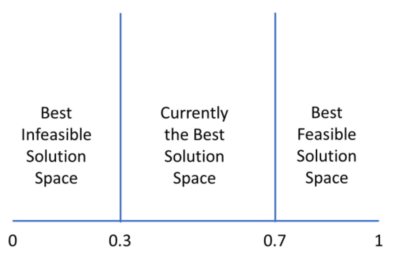
• Regarding the demand bidding planning of the user aggregators, the demand planning strategy for maximum profit can be formulated as follows:

  $$\underset{p_1,\cdots p_T}{\mathrm{maximize}}{\displaystyle \sum _{t=1}^T({\lambda }_t^{\mathrm{est}}{p}_t-{\displaystyle \sum _{n=1}^N{U}_{t,n}Fc{t}_{t,n}^{}})}\hspace{0.17em},\hspace{0.17em}{p}_1,\cdots ,p_T\in \mathrm{\Pi }$$

  (7)

  $$Fc{t}_n=a_{n}Pc{t}_n^2+b_n^{}Pc{t}_n^{}+c_n^{}$$

  (8)

  where $U_{t,n}$ is the purchase status of the user aggregators for downstream users during the period $t$. $Fc{t}_{t,n}^{}$ and $Pc{t}_n^{}$ are the cost function and electricity amount of the user aggregators in the demand bidding, respectively. $a,\hspace{0.17em}b$, and $c$ are the demand bidding curves of user aggregators. $\mathrm{\Pi }$ is a feasible solution. $N$ is the number of user aggregators who took part in the demand bidding during the time period $t$. The demand bidding must face the tradeoff between the maximum profit and the minimum risk. If the user aggregators seek to minimize risk regardless of profit, the risk minimization procedure can be formulated as follows:

  $$\underset{p_1,\cdots p_T}{\mathrm{minimize}}{\displaystyle \sum _{i=1}^T{\displaystyle \sum _{j=1}^T{p}_i{V}_{ij}^{\mathrm{est}}{p}_j}}\hspace{0.17em}\hspace{0.17em},\hspace{0.17em}{p}_1,\cdots ,p_T\in \mathrm{\Pi };$$

  (9)
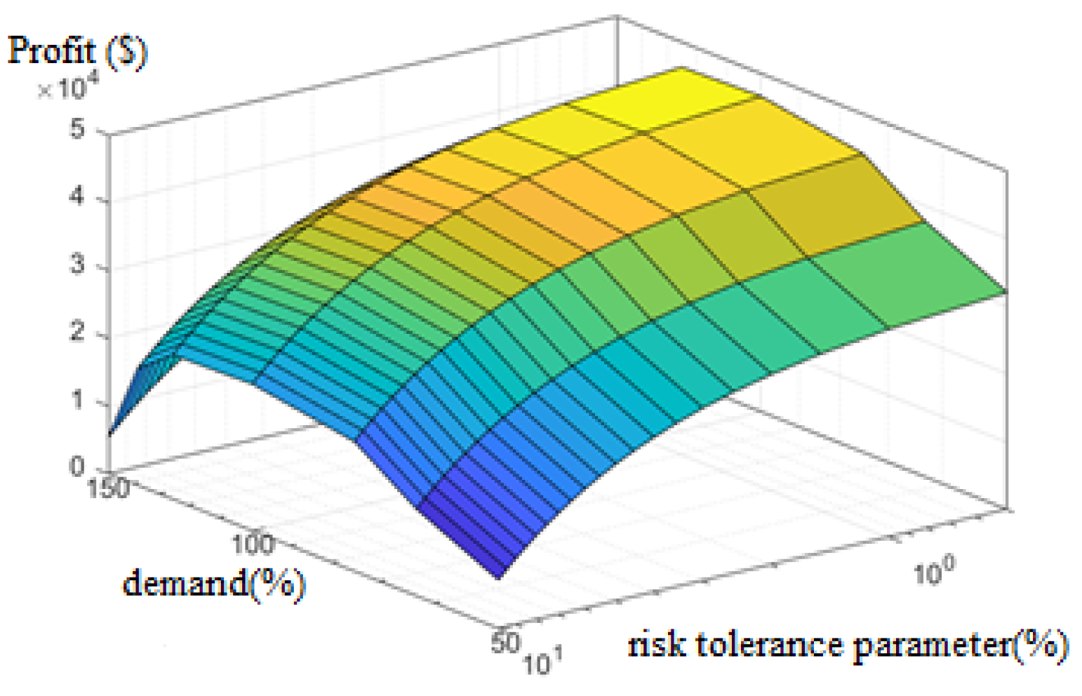
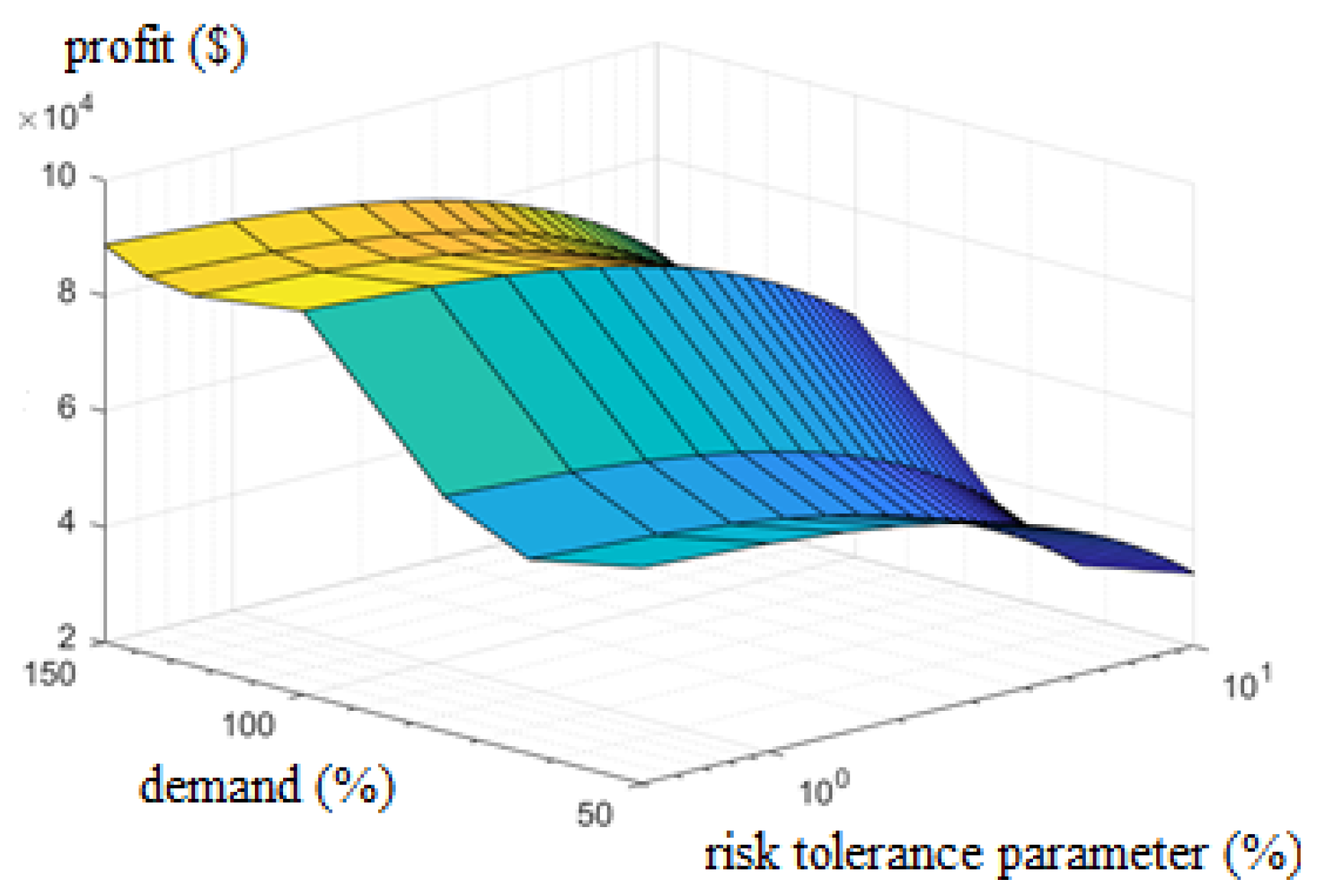
• $V^{\mathrm{est}}$ is the risk variation of the demand price of the utility during the peak hours, while $p_i$ and $p_j$ are the demand bids by the user aggregators. The user aggregators are most interested in the best demand bidding to make profits, and the demand bidding of these user aggregators have the maximum profit with the minimum risk. In order to compromise these two conflicting goals, the best choice is complemented by a risk-tolerance parameter $\beta$. Therefore, the demand bidding for the user aggregators, taking both risk and maximum profit into consideration, can be formulated as Equation (10):

  $$\underset{p_1,\cdots p_T}{\mathrm{maximize}}{\displaystyle \sum _{t=1}^T({\lambda }_t^{\mathrm{est}}{p}_t-{\displaystyle \sum _{i=1}^N{U}_{t,i}Fc{t}_{t,i}^{}})}-\beta {\displaystyle \sum _{i=1}^T{\displaystyle \sum _{j=1}^T{p}_i{V}_{ij}^{\mathrm{est}}{p}_j}},\hspace{0.17em}{p}_1,\cdots ,p_T\in \mathrm{\Pi }$$

  (10)

  in addition, it should meet the restriction conditions of period $t$ as in Equation (11):

  $${\displaystyle \sum _{n=1}^N{U}_{t,n}Fc{t}_{t,n}^{}}=P_{t,i}\hspace{1em}t=1,2,\dots ,T$$

  (11)

  profit and risk are two different objectives. Hence, a compromise solution is required to solve the demand bidding problem. Equation (10) is an objective function in this paper. The objective function adopted the concepts of “profit” and “risk” to obtain the maximum profit by controlling the “risk”. When the risk-tolerance parameter $\beta$ is higher, the profit is lower.

3. Feasible Particle Swarm Optimization

In 1995, PSO was developed by [24] to simulate numerical analysis. The PSO algorithm is based on the mechanism of birds’ swarming behavior. When birds forage, each bird is like a particle. Each particle keeps in mind its current best position ($pbest$), and the best position of the group (gbst) in the population. The disadvantage of PSO is that the convergence speed is higher in the initial search for solving the optimization problem. In the later stage, the particle swarm gradually moves toward the optimal solution of the swarm. Thus, the diversity of the whole swarm is lost, and the particle can easily fall into the local optimal solution.

In PSO, the position and velocity of particles are defined in Equations (12) and (13):

$$v_i^{t+1}=w\times v_i^t+c_1\times rand\times (pbes{t}_i^t-x_i^t)+c_2\times rand\times (gbes{t}_{}^t-x_i^t)$$

(12)

$$x_i^{t+1}=x_i^t+v_i^{t+1}$$

(13)

where $x_i^t$ is the position of particle $i$ at iteration $t$, and $v_i^t$ is the velocity of particle $i$ during iteration $t$. $pbes{t}_i^t$ is the best position of a particle $i$ at iteration $t$, and $gbes{t}_{}^t$ is the best position of all particles at iteration $t$. $c_1$ and $c_2$ are learning constants that influence the forward speed of the particle. In this paper, $c_1$ and $c_2$ are 2.05. $w$ is the speed weight of the current generation, and $w$ means a small variance when the particle changes its position; otherwise, the variance is large.

PSO has the characteristics of movement, evolution, elimination, and multiple variability. The movement in the PSO process is only dependent on the movement distance generated, and the movement information is transmitted between the particles. It is easy to converge on the local optimum. FPSO introduces an auto-tuning scheme that allocates “infeasible solution ($gbes{t}_{\inf }$)” and “feasible solution ($gbes{t}_{\mathrm{f}}$)” to the solution space by using random parameters to make the PSO search for the global optimum more efficient, as shown in Figure 1. In Figure 1, the “infeasible solution ($gbes{t}_{\inf }$)” space may be an attractive solution in the next generation, and improvement of the auto-tuning solution starts with finding the best direction to take advantage of more opportunity to obtain the global optimum. The velocity of particles in the FPSO system is defined in Equation (14):

$$\begin{array}{ccc}if& r<0.3& \\ & then& \begin{array}{cc}\hfill v_{i,j}^{t+1}& =w\times v_{i,j}^t+c_1\times rand\times (pbes{t}_{i,j}^{}-x_{i,j}^t)\hfill \\ & +c_2\times rand\times (gbes{t}_{\inf ,j}^{}-x_{i,j}^t)\hfill \end{array}\\ elseif& 0.3\le r\le 0.7& \\ & then& \begin{array}{cc}{v}_{i,j}^{t+1}& =w\times v_{i,j}^t+c_1\times rand\times (pbes{t}_{i,j}^{}-x_{i,j}^t)\hfill \\ & +c_2\times rand\times (gbes{t}_j^{}-x_{i,j}^t)\hfill \end{array}\\ else& r>0.7& \\ & then& \begin{array}{cc}{v}_{i,j}^{t+1}& =w\times v_{i,j}^t+c_1\times rand\times (pbes{t}_{i,j}^{}-x_{i,j}^t)\hfill \\ & +c_2\times rand\times (gbes{t}_{f,j}^{}-x_{i,j}^t)\hfill \end{array}\end{array}$$

(14)

Figure 2 presents a flowchart of the solution algorithm.

4. Case Study and Analysis

In this paper, the utility firm purchased demand from user aggregators for a total of 6 h. The demand price announced by the utility firm is shown in

Table 1. Demand price (USD/MW).

Hour	10	11	13	14	15	16
Price	66.609	78.372	85.698	78.273	72.072	63.342

, and the demand to be provided after the bidding is shown in

Table 2. Demand provided of user aggregators.

Hour	10	11	13	14	15	16
DR(MW)	352.81	364.18	417.69	396.41	387.3795	370.56

. The model of the covariance matrix constructed by the user aggregators with the use of the bidding history data of the demand trading market is shown in

Table 3. Covariance matrix of electricity prices.

Hour	10	11	13	14	15	16
10	0.0036	−0.0018	0.0054	−0.0036	−0.0018	0.0018
11	−0.0018	0.0009	−0.0027	0.0018	0.0009	−0.0009
13	0.0054	−0.0027	0.0081	−0.0054	−0.0027	0.0027
14	−0.0036	0.0018	−0.0054	0.0036	0.0018	−0.0018
15	−0.0018	0.0009	−0.0027	0.0018	0.0009	−0.0009
16	0.0018	−0.0009	0.0027	−0.0018	−0.0009	0.0009

[25]. In addition, the risk-tolerance parameter was set as β = 0.05; the higher β has the lower the revenue of the user aggregators. After predicting the demand price of the utility firm, the covariance matrix is constructed, and the risk-tolerance parameter is set so that the profit maximization of the user aggregators with risk assessment can be calculated.

Two cases with a demand bidding curve for user aggregators are analyzed to assess the feasibility of the proposed algorithm. The two cases are expressed as:

Case 1.

Profit maximization of the user aggregators with the quadratic bidding curve;

Case 2.

Profit maximization of the user aggregators with different bidding curves.

All data were obtained from TPC Power Development Planning [26].

Case 1.

Profit maximization of the user aggregators with the quadratic bidding curve.

In this case, 13 user aggregators were taken as samples using the quadratic bidding curve.

Table 4. Bidding curve of user aggregators.

Aggregator	Max. (MW)	Min. (MW)	a	b	C
1	17.1	3	0.69	33.65	9.4705
2	28.5	5	0.942	40.9	36.903
3	45	5	0.357	40.15	28.771
4	45	5	0.605	64.5	0
5	75	10	0.421	62.5	91.34
6	75	10	0.708	45.75	172.83
7	82.5	15	0.313	39.85	64.783
8	82.5	30	0.298	33.15	78.596
9	82.5	30	0.277	35.5	80.132
10	22.5	4	0.52124	16.65	105.51
11	28.5	5	0.16	32.15	22.292
12	30	5	0.01	44.75	10.787
13	16.5	3	1.61	29.4	30.745

shows the parameter coefficients of the bidding curve for the user aggregators.

FPSO is used to optimize the amount and price of bidding demand as shown in

Table 5. Bidding demand amount and price in Case 1.

Unit	Demand Amount (MW/hour)						Total (MW)	Total Purchase Price (USD)	Purchase Price Per Unit (USD/MW)
	10	11	13	14	15	16
1	17.09	17.10	17.10	17.05	17.10	17.07	102.52	4715.04	45.99
2	16.34	15.63	18.04	17.11	18.22	14.83	100.17	5902.04	58.92
3	42.37	45.00	45.00	44.90	45.00	45.00	267.27	15,155.67	56.71
4	0	0	0	0	0	0	0	0	0
5	0	0	0	0	0	0	0	0	0
6	13.65	19.80	23.19	21.32	22.71	16.94	117.61	8097.63	68.85
7	42.57	42.97	59.50	54.15	46.93	47.21	293.33	16,635.63	56.71
8	63.96	71.16	82.50	68.97	72.71	65.05	424.35	23,549.40	55.49
9	62.92	59.43	75.17	76.31	69.79	69.21	412.82	23,064.65	55.87
10	22.50	22.50	22.50	22.50	22.39	22.50	134.89	4459.83	33.06
11	28.50	28.50	28.50	28.50	28.50	28.34	170.84	6404.57	37.49
12	30.00	29.94	30.00	29.92	30.00	30.00	179.86	8167.34	45.41
13	12.10	11.97	16.50	15.28	14.65	13.87	84.35	4599.60	54.53

. Because the demand prices for users 4 and 5 are relatively high, they have no winning bids. In these 6 h, the demand price provided by the utility firm to the user aggregators is USD 170,192.1, and the risk cost calculated by the V^est covariance matrix and the risk tolerance parameter β = 0.05 is USD 13,078.08. The demand purchase cost paid by the user aggregators to the downstream users is USD 120,741, and the average purchase price per unit is USD 52.78 MW. Therefore, the maximum profit of the user aggregators with risk assessment is USD 34,793.28.

When the demand purchase is a quadratic curve, the demand purchase amount of the user aggregators also affects the profit directly. When the sum of demands in Table 5 is 100%, the cases of 50% and 150% demand are calculated. The profit of the user aggregators is shown in Figure 3. When the risk tolerance parameter β = 0.05, the profit at 50% demand is USD 20,314.10, and the profit at 150% demand is USD 18,363.59. Both of them are less than the profit of 100% demand, which is USD 34,793.28. Therefore, it could be found that the user aggregators must effectively evaluate the purchase cost of downstream users and select the appropriate demand to provide while participating in the purchase from the utility firm.

Case 2.

Profit maximization of the user aggregators with different bidding curves.

The user aggregators consisted of 13 users. The bidding curves are linear, quadratic, and segment linear, as shown in Figure 4, and their detailed data parameters are shown in

Table 6. Bidding curves of the different user aggregators.

Aggregator	1	2	3	4	5	6	7
Max.	17.1	28.5	45	45	75	75	82.5
Min.	3	5	5	5	10	10	15
A	0	0.942	0	0	0.421	0	0
b1	33.65	40.9	40.15	64.5	62.5	45.75	39.85
C	9.4705	36.903	28.771	72.282	91.34	172.83	64.783
b2	0	0	48.18	0	0	54.9	0
Not Operate Min.			23			40
Not Operate Max.			27			45
Aggregator		8	9	10	11	12	13
Max.		82.5	82.5	22.5	28.5	30	16.5
Min.		30	30	4	5	5	3
A		0.298	0	0	0.16	0	0
b1		33.15	35.5	16.65	32.15	44.75	29.4
C		78.596	80.132	105.51	22.292	10.787	30.745
b2		0	42.6	0	0	53.7	0
Not Operate Min.			54			16
Not Operate Max.			59			19

The operating curve of aggregators 1, 4, 7, 10, and 13 is a linear function. The operating curve of aggregators 2, 5, 8, and 11 is a quadratic function. The operating curve of aggregators 3, 6, 9, and 12 is a segment linear function.

. Users 3, 6, 9, and 12 are segmented linearly with forbidden zones, and purchase demand could not be purchased from them between the minimum and maximum non-operational zones.

Table 7. Bidding demand amount and price in Case 2.

Unit	The Demand Amount (MW/Hour)						Total (MW)	Total Purchase Price (USD)	Purchase Price Per Unit (USD/MW)
	10	11	13	14	15	16
1	17.10	15.65	17.10	17.08	17.09	17.10	101.12	3459.43	34.21
2	0.00	0.00	14.77	0.00	0.00	0.00	14.77	846.80	57.32
3	45.00	44.40	45.00	45.00	45.00	44.97	269.37	10,934.02	40.59
4	0	0	0	0	0	0	0	0	0
5	0	0	0	0	0	0	0	0	0
6	38.83	75.00	75.00	75.00	75.00	64.84	403.67	18,090.70	44.82
7	81.13	82.50	82.50	82.50	82.50	82.50	493.63	20,059.66	40.64
8	54.73	43.36	52.08	46.85	40.86	34.65	272.52	13,276.11	48.72
9	47.72	35.79	53.87	53.92	53.35	52.94	297.59	12,120.89	40.73
10	22.50	22.50	22.50	22.50	22.50	22.50	135.00	2880.81	21.34
11	28.50	28.29	28.50	28.50	28.50	28.50	170.79	6402.65	37.49
12	0	0	10.18	8.15	6.69	5.54	30.57	2260.65	73.96
13	16.50	16.50	16.50	16.50	16.50	16.47	98.97	3094.24	31.26

shows the amount and price of bidding demand. In Table 7, the bidding curves of users 4 and 5 were relatively high, while the cost of user 12 became expensive in the later period. In these 6 h, the demand purchase price provided by the utility firm to the user aggregators is USD 170,192.1, and the risk cost calculated by the V^est covariance matrix and the risk tolerance parameter β = 0.05 is USD 13,078.07. The demand purchase cost paid by the user aggregators to the downstream users is USD 93,795.15. Therefore, the maximum profit of the user aggregators with risk assessment is USD 74,673.67. Because Case 1 has a quadratic purchase curve, the profit of Case 2 is higher than that of Case 1.

When the demand purchase curve is different, the demand purchase amount of the user aggregators will also affect the profit directly. When the sum of demand shown in Table 7 was 100%, the cases of 50% and 150% demand were calculated. The profit of the user aggregators is shown in Figure 5. The profit of 50% demand is USD 45,700.71, the profit of 100% demand is USD 74,673.67, and the profit of 150% demand is USD 77,030.91. It was found that the profit of the DR user aggregators at 100% and 150% became gradually flat and could not generate more profit.

Based on the measurement formulas of Case 1 and Case 2, it can be seen that different user demand purchase curves had a great influence on the profit of the user aggregators. Therefore, the proportion of the user aggregators that participate in the demand purchase by the utility firm also needs to be effectively evaluated to calculate the maximum profit value for the user aggregators.

5. Conclusions

This study mainly discussed the demand bidding model of user aggregators and considered the maximum profit after taking profit and risk into consideration. The covariance matrix of demand prices was used to establish the demand price variability and derive the risk model of demand bidding. By using a risk-tolerance parameter β, a new demand bidding model for the user aggregators that takes both risk and profit into consideration was formulated. All constraints, including the load balance and bidding capacity constraints, were considered in this paper. This paper used Feasible Particle Swarm Optimization (FPSO) to perform simulations and analyses. Two cases with different bidding curves of user aggregators were used to simulate the efficiency of the proposed algorithm. We found that the user aggregators can effectively select the appropriate risk and demand during the bidding procedure. It is believed that the proposed algorithms could provide relevant practitioners with a simple and rapid tool to cope with possible uncertain electric price changes in the future and improve the practitioners’ abilities in managing dispatching risks and making cost evaluations, as well as generating capability constraints.

References

1. Taiwan Power Company. Available online: http://www.taipower.com.tw/content/new_info/ (accessed on 1 April 2022).
2. Taiwan Power Company. Time-of-Use Rate for Industry. Available online: http://www.taipower.com.tw/electricity (accessed on 1 April 2022).
3. Glazunova, A. Development of a Day-Ahead Demand Side Management Strategy to Improve the Microgrid Efficiency. IFAC-Papers OnLine 2022, 55, 256–261. [Google Scholar] [CrossRef]
4. Chung, C.Y. The study of the electricity analysis and demand response strategy of shopping malls. Master’s Thesis, Cheng-Shing University, Kaohsiung, Taiwan, 2021. [Google Scholar]
5. Pasetti, M.; Rinaldi, S.; Manerba, D. A virtual plant architecture for the demand-side management of smart prosumers. Appl. Sci. 2018, 8, 432. [Google Scholar] [CrossRef] [Green Version]
6. Duan, Q. A price-based demand response scheduling model in day-ahead electricity market. In Proceedings of the 2016 IEEE Power and Energy Society General Meeting (PESGM), Boston, MA, USA, 17–21 July 2016. [Google Scholar]
7. Safar, A.; Tahmasebi, M.; Pasupuleti, J. Smart buildings aggregator bidding strategy as a negawatt demand response resources in the spinning reserve electricity market. In Proceedings of the 2019 IEEE PES Innovative Smart Grid Technologies Europe (ISGT-Europe), Bucharest, Romania, 29 September–2 October 2019. [Google Scholar]
8. Jia, Y.; Mi, Z.; Yu, Y.; Song, Z.; Liu, L.; Sun, X. Purchase bidding strategy for load agent with the incentive-based demand response. IEEE Access 2019, 7, 58626–58637. [Google Scholar] [CrossRef]
9. Dadashi, M.; Haghifam, S.; Zare, K.; Haghifam, M.R.; Abapour, M. Short-term scheduling of electricity retailers in the presence of Demand Response Aggregators: A two-stage stochastic bi-Level programming approach. Energy 2020, 205, 117926. [Google Scholar] [CrossRef]
10. Abapour, S.; Mohammadi, B.; Hagh, M.T. Robust bidding strategy for demand response aggregators in electricity market based on game theory. J. Clean. Prod. 2020, 243, 118393. [Google Scholar] [CrossRef]
11. Liu, X.; Li, Y.; Lin, X.; Guo, J.; Shi, Y.; Shen, Y. Dynamic bidding strategy for a demand response aggregator in the frequency regulation market. Appl. Energy 2022, 314, 118998. [Google Scholar] [CrossRef]
12. Li, S.; Zhang, L.; Nie, L.; Wang, J. Trading strategy and benefit optimization of load aggregators in integrated energy systems considering integrated demand response: A hierarchical Stackelberg game. Energy 2022, 249, 123678. [Google Scholar] [CrossRef]
13. Pourramezan, A.; Samadi, M. A novel approach for incorporating incentive-based and price-based demand response programs in long-term generation investment planning. Int. J. Electr. Power Energy Syst. 2022, 142, 108315. [Google Scholar] [CrossRef]
14. Tang, W.; Yang, H.T. Optimal operation and bidding strategy of a virtual power plant integrated with energy storage systems and elasticity demand response. IEEE Access 2019, 7, 79798–79809. [Google Scholar] [CrossRef]
15. Dahraie, M.V.; Kermani, H.R.; Moghadda, A.A. Risk-averse probabilistic framework for scheduling of virtual power plants considering demand response and uncertainties. Int. J. Electr. Power Energy Syst. 2020, 121, 106126. [Google Scholar] [CrossRef]
16. Liang, Z.; Alsafasfeh, Q.; Jin, T.; Pourbabak, H.; Su, W. Risk-constraints optimal energy management for virtual power plants considering correlated demand response. IEEE Trans. Smart Grid 2019, 10, 1577–1587. [Google Scholar] [CrossRef]
17. Zare, K.; Nojavan, S. Risk-based optimal bidding strategy of generation company in day-ahead electricity market using information gap decision theory. Int. J. Electr. Power Energy Syst. 2013, 147, 83–92. [Google Scholar]
18. Kim, H.J.; Kim, M.K. Risk-based hybrid energy management with developing bidding strategy and advanced demand response of grid-connected microgrid based on stochastic/information gap decision theory. Int. J. Electr. Power Energy Syst. 2021, 131, 107046. [Google Scholar] [CrossRef]
19. Tian, M.T.; Yan, S.R.; Tian, X.T.; Nojavan, S.; Jermsittiparsrt, K. Risk and profit-based bidding and offering strategies for pumped hydro storage in the energy market. J. Clean. Prod. 2020, 256, 120715. [Google Scholar] [CrossRef]
20. Fazlalipour, P.; Ehsan, M.; Mohammadi-Ivatloo, B. Risk-aware stochastic bidding strategy of renewable micro-grids in day-ahead and real-time markets. Energy 2019, 171, 689–700. [Google Scholar] [CrossRef]
21. Alexander, C. Risk Management and Analysis- Volume 1 Measuring and Modeling Financial Risk; John Wiley & Sons Ltd.: Hoboken, NJ, USA, 2000. [Google Scholar]
22. Taiwan Power Company. The Demand Response Load Management Strategy. Available online: https://www.taipower.com.tw/tc/news2.aspx (accessed on 15 December 2021).
23. Lucas, A.; Zhang, X. Score-driven exponentially weighted moving averages and Value-at-Risk forecasting. Int. J. Forecast. 2016, 32, 293–302. [Google Scholar] [CrossRef] [Green Version]
24. Kennedy, J.; Eberhart, R.C. Particle Swarm Optimization. In Proceedings of the IEEE International Conference on Neural Networks, Perth, WA, Australia, 27 November–1 December 1995; Volume 4, pp. 1942–1948. [Google Scholar]
25. Lin, W.M.; Gow, H.J.; Tsai, M.T. Electricity Price Forecasting Using Enhanced Probability Neural Network. Energy Convers. Manag. 2010, 51, 2707–2714. [Google Scholar] [CrossRef]
26. Taiwan Power Company. The Sustainable Operation of White Paper for Taiwan Power Company; Taiwan Power Company: Taipei, Taiwan, 2021. [Google Scholar]
Figure 1. The auto-tuning scheme of FPSO.
Energies 16 00156 g001
Figure 2. Flowchart of the solution algorithm.
Energies 16 00156 g002
Figure 3. Profit diagram of bidding demand in Case 1.
Energies 16 00156 g003
Figure 4. Bidding curves of user aggregators in Case 2.
Energies 16 00156 g004
Figure 5. Profit diagram of bidding demand in Case 2.
Energies 16 00156 g005