Numerical Investigation on the Effects of Wind and Shielding Conductor on the Ion Flow Fields of HVDC Transmission Lines

Abstract

Ion flow field is an important aspect of high voltage direct current (HVDC) transmission lines. In this paper, we apply the upwind finite volume method for solving the ion flow field of three HVDC configurations to clarify the effect of the wind and the role of shielding conductors. For the monopolar configuration installation, the ground current distribution with underbuilt shield wires was studied numerically and experimentally. For the ±250 kV bipolar configuration, the calculated peak electric field and current density are verified with the values in a reference. The ±500 kV bipolar configuration is used to investigate the change in electric field and ion current within the same corridors of the existing HVAC lines. We analyze the ion flow field with and without the dedicated metallic return conductor (DMRC). In the absence of wind, the maximum of the electric field is lower than that of the HVAC lines and the current density is very low on the ground. In the presence of wind, the electric field and the current distribution become unsymmetrical on the ground level. The peak current density increases significantly on the downwind side. The HVDC line without DMRC has the electric field peak higher than that of the HVAC lines. With the higher wind shear coefficient, the peak of the electric field and the current density increases on the downwind side. Overall investigations summarize that DMRC can effectively reduce the peak of the electric field to be lower than that of the existing 500 kV HVAC lines under all wind conditions.

1. Introduction

Corona discharge at the energized conductors of HVDC transmission lines generates ions continuously from the lines. Ions migrate from their corresponding conductors to the oppositely polarized conductor or to the ground, depending on the drift and diffusion motion. The ion flow field distribution between the conductors and the ground plane can be influenced by environmental conditions. Transverse wind is possibly a significant external factor affecting the ion movement towards the ground plane for overhead HVDC lines. Therefore, for the evaluation of the ground-level electric field and ion current density under the overhead lines, we need to consider the environmental impact in addition to the HV conductor configurations.

The influence of wind on HVDC transmission lines has been the focus of many studies. Numerical simulations and experimental measurements have been employed to analyze the space charges and their motion in reduced-scale and full-scale models. In early works, outdoor experiments under different wind and applied voltage conditions were performed to investigate the relationship between the electric field and the current density distributions at the ground level [1]. The profile measurements on a steel plane under HVDC conductors used the field meters detecting the electric field and the current probes recording the ion current. The experiments were carried out under two conditions: the condition without wind and the condition with forced wind. For the case of the monopolar line with corona discharge, the ground electric field was reduced slightly but the profile of the current density on the ground significantly changed. The peak values of the current density increased due to wind. For the bipolar lines, the electric field magnitude was similar to that of the monopolar line; however, the current density profile increased and decreased on the downwind and upwind sides, respectively. The ionic current region could be extended significantly, depending on the wind condition.

The ion flow field has been simulated by various numerical methods. The upstream finite element method (FEM) was developed to calculate the electric field and ion current density profiles in the presence of wind. The upstream FEM applied the current continuity equation in an integral form and gave highly stable calculations. The calculated profiles on the ground agreed with the measurement results in the laboratory and those of UHVDC test lines [2]. The effect of wind was considered in the flux tracing method for the ±900 kV bipolar line with bundled conductors [3]. The results showed that the patterns and termination of flux lines on sub-conductor surfaces changed with transverse wind. Onsite statistical measurements of the ground electric field and the ion current density were conducted under ±800 kV UHVDC operating transmission lines to correlate the impact of transverse wind velocities with the ionized field [4]. The measured results were consistent with the simulation using the finite volume method (FVM), which considered the corona inception criteria by photoionization and photoemission.

Existing works on the effects of wind on HVDC transmission lines have been expanded to include the time-varying characteristics of wind and the factors that influence wind speed. Based on the time series model and the Kalman filter method, short-term wind speed was used to predict the ion flow [5]. The simulation was done by the FEM and time-domain FVM method. The results agreed with long-term statistical measured data. The ion current density and the electric field dynamics on the ground level were significantly influenced by the wind. In the case of very strong wind, space charges were blown away and had no effect on the total electric field at ground level. Atmospheric stability factors were applied to calculate the height-dependent wind speed with a power law profile model [6]. The height-dependent wind was applied to the ion flow model for large-scale transmission lines. The transverse wind speed changed the charge distribution. The electric field and the ion current were indirectly affected by the atmospheric conditions.

Despite a number of studies on wind factors, the local topography of each country has an impact on the complex wind characteristics. The variations in HVDC configuration design may also result in the different ion flow environment. The influence of shielding wires was analyzed in the absence of wind [7,8]. The single wire with different locations was evaluated on the ion field distribution to study the shielding effectiveness. An interconnection link between Thai and Malaysian grids has been operated since 2002 [9]. For the installation of ±500 kV HVDC interconnecting lines in north and north-eastern Thailand, the conversion of existing 500 kV HVAC grids to the HVDC ones is under consideration due to difficulties in obtaining right of way (ROW) permission [10]. Therefore, a study on the ion flow field of the HVDC transmission lines for such converted configuration is of high practical interest. The effects of shielding bundled conductors and wind parameter can be fulfilled for the HVDC studies.

In this paper, we analyze the ion flow field of the ±500 kV HVDC transmission lines that are to be converted from an existing 500 kV HVAC. The object of the study is to investigate the change in the ground level electric field and the ion current, which is trivial under the HVAC lines. The configurations of ±500 kV HVDC with and without the installation of dedicated metallic return conductors (DMRC) are treated to clarify the effects on the field. The effect of wind on the ground ion current density of the HVDC lines is analyzed. We apply the upwind FVM method for the analysis. We utilize a fluid dynamic software (ANSYS FLUENT) to solve the problem. The wind data and wind shear coefficient observed in Thailand are treated in the calculation. We also conducted an experiment with a reduced-scale model having various underbuilt shield wires to validate the calculation results.

2. Methodology

2.1. Ion Flow Field Equations

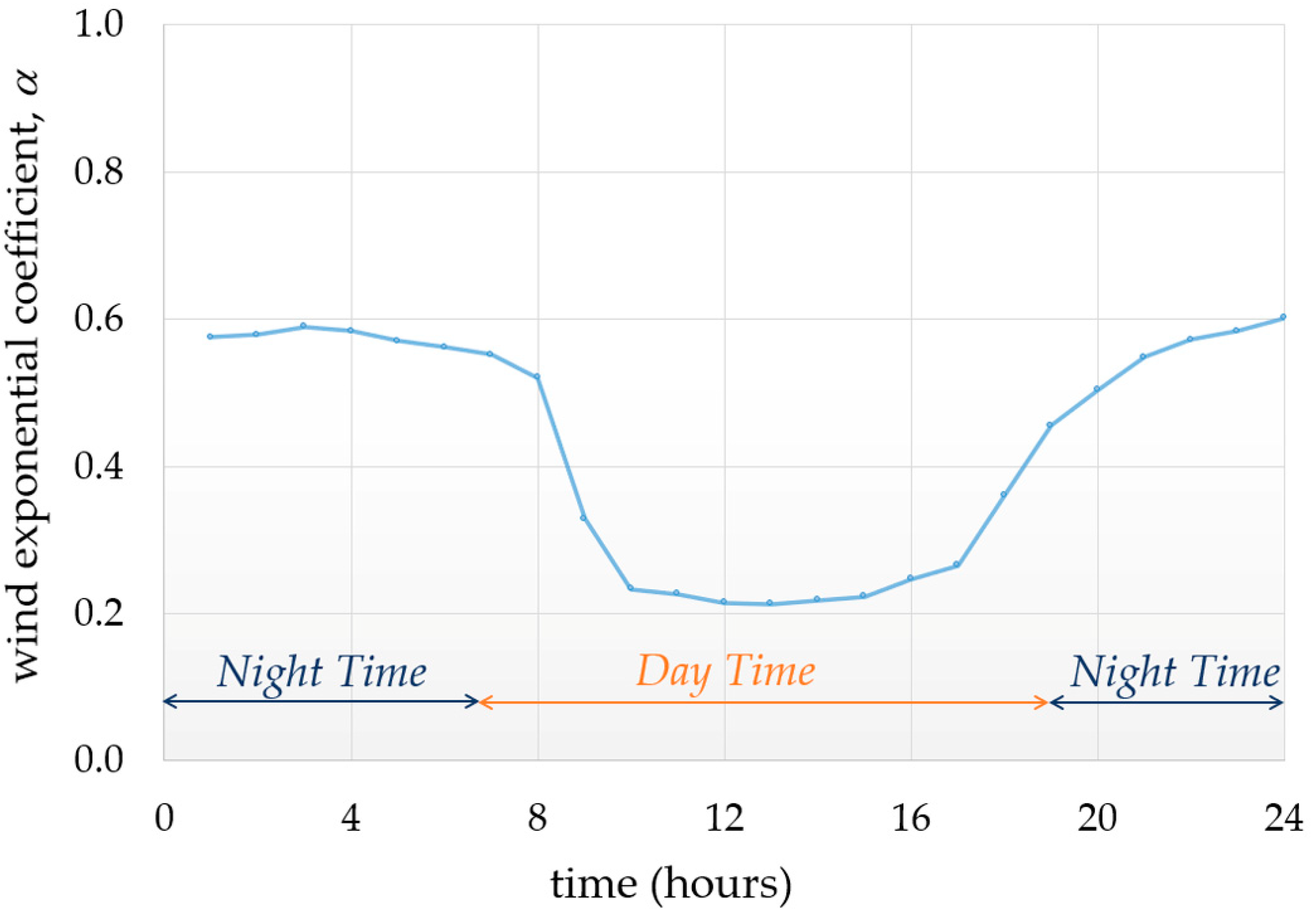
For HVDC transmission lines, the ions modify the electric field and contribute to the ion current. The current flows in the space between the conductors of opposite polarities and between the lines and the ground. The relationship between the ions and the electric field is described by Poisson’s equation. At time $t$, electric field $\mathbf{E}\left(t\right)$, electric potential $V\left(t\right)$, positive ion density ${\rho }_{+}\left(t\right)$, and negative ion density ${\rho }_{-}\left(t\right)$ follow the relationship [11]

$$\nabla \mathbf{E}\left(t\right) = \frac{{\rho }_{+}\left(t\right) - {\rho }_{-}\left(t\right)}{{\epsilon }_0} \mathrm{or} - {\nabla }^{2}V\left(t\right) \frac{{\rho }_{+}\left(t\right) - {\rho }_{-}\left(t\right)}{{\epsilon }_0}$$

(1)

where the permittivity of air ${\epsilon }_0$ equal to 8.854 × 10⁻¹² F/m.

The movement of ions due to the electric field and wind velocity $\mathbf{w}\left(t\right)$ results in ion current densities ${\mathbf{J}}_{+}\left(t\right)$ and ${\mathbf{J}}_{-}\left(t\right)$, which are expressed by

$${\mathbf{J}}_{+}\left(t\right) = {\mu }_{+}{\rho }_{+}\left(t\right) \mathbf{E}\left(t\right) - D_{+}\nabla {\rho }_{+}\left(t\right) + {\rho }_{+}\left(t\right) \mathbf{w}\left(t\right)$$

(2)

$${\mathbf{J}}_{-}\left(t\right) = {\mu }_{-}{\rho }_{-}\left(t\right) \mathbf{E}\left(t\right) + D_{-}\nabla {\rho }_{-}\left(t\right) - {\rho }_{-}\left(t\right) \mathbf{w}\left(t\right)$$

(3)

where μ is the ion mobility and D is the ion diffusion coefficient. The subscripts + and − are consistently used to associate the properties with the positive and negative ions in this paper.

The continuity equations for the ions are

$$\frac{\partial {\rho }_{+}\left(t\right)}{\partial t}+\nabla ·{ \mathbf{J}}_{+}\left(t\right) = -R \frac{{\rho }_{+}\left(t\right) {\rho }_{-}\left(t\right)}{e}$$

(4)

$$\frac{\partial {\rho }_{-}\left(t\right)}{\partial t}-\nabla ·{ \mathbf{J}}_{-}\left(t\right) = -R \frac{{\rho }_{+}\left(t\right) {\rho }_{-}\left(t\right)}{e}$$

(5)

where R is the recombination coefficient and e is the elementary charge of an electron.

Substituting the ${\mathbf{J}}_{+}\left(t\right)$ and ${\mathbf{J}}_{-}\left(t\right)$ from Equations (2) and (3) into Equations (4) and (5), we obtain the governing equations for the charge transportations

$$\frac{\partial {\rho }_{+}\left(t\right)}{\partial t}+\nabla ·{\rho }_{+}\left(t\right) \left[{\mu }_{+}\mathbf{E}\left(t\right)+\mathbf{w}\left(t\right)\right]-D_{+}{\nabla }^2{\rho }_{+}\left(t\right)=-R\frac{{\rho }_{+}\left(t\right) {\rho }_{-}\left(t\right)}{e}$$

(6)

$$\frac{\partial {\rho }_{-}\left(t\right)}{\partial t}+\nabla ·{\rho }_{-}\left(t\right) \left[-{\mu }_{-}\mathbf{E}\left(t\right)+\mathbf{w}\left(t\right)\right]-D_{-}{\nabla }^2{\rho }_{-}\left(t\right)=-R\frac{{\rho }_{+}\left(t\right) {\rho }_{-}\left(t\right)}{e}$$

(7)

2.2. Wind Profiles

Wind characteristics vary with space, time, and the local geographical area and the weather condition. Due to wind shear, the average wind velocity rises with the height above the ground. Therefore, we express the wind velocity as a function of height for the calculation in this paper. We adapt the power law (often used due to its simplicity) to model the wind profile. Based on the power law, the wind velocity $w_h$ at height h above the ground level is described as [12]

$$w_h=w_r{\left(\frac{h}{h_r}\right)}^{\alpha }$$

(8)

Figure 1 shows the 24-h variation wind data for Khon Kaen province in the northeastern region of Thailand. The average wind velocity is applied with $w_r$ = 1.3 m/s. The annual data are obtained from the Thai Meteorological Department. The α characteristics are obtained from measured data [13]. The annual average α is approximately 0.4; however, α varies between 0.2 to 0.6 during the hours of the day, as shown in Figure 1. In this paper, we take the variation of α into account to evaluate the relationships between α and the electric field and ion current at the ground level.

2.3. Charge Initialization

For the initialization of charge in the calculation domain, we set an ionization layer enclosing each energized conductor. Space charges are produced by corona discharge in the layer if the electric field exceeds the corona-onset value $E_C$, which is expressed as [14]

$$E_C = m A \delta \left[1+\frac{B}{\sqrt{{\delta r}_{\mathit{cond}}}} \right]$$

(9)

where m is the irregularity factor of the conductor surface (m = 0.9 for the monopolar reduced scale model and 0.7 for the stranded conductor of the bipolar line models), $\delta$ is the relative air density factor and $r_{\mathit{cond}}$ is the radius of the conductor in cm. A and B are the empirical constants depending on the voltage polarity. For positive voltages, A = 33.7 kV/cm and B = 0.24 cm^1/2. For negative voltages, A = 31.0 kV/cm and B = 0.308 cm^1/2. $\delta$ is taken to be unity.

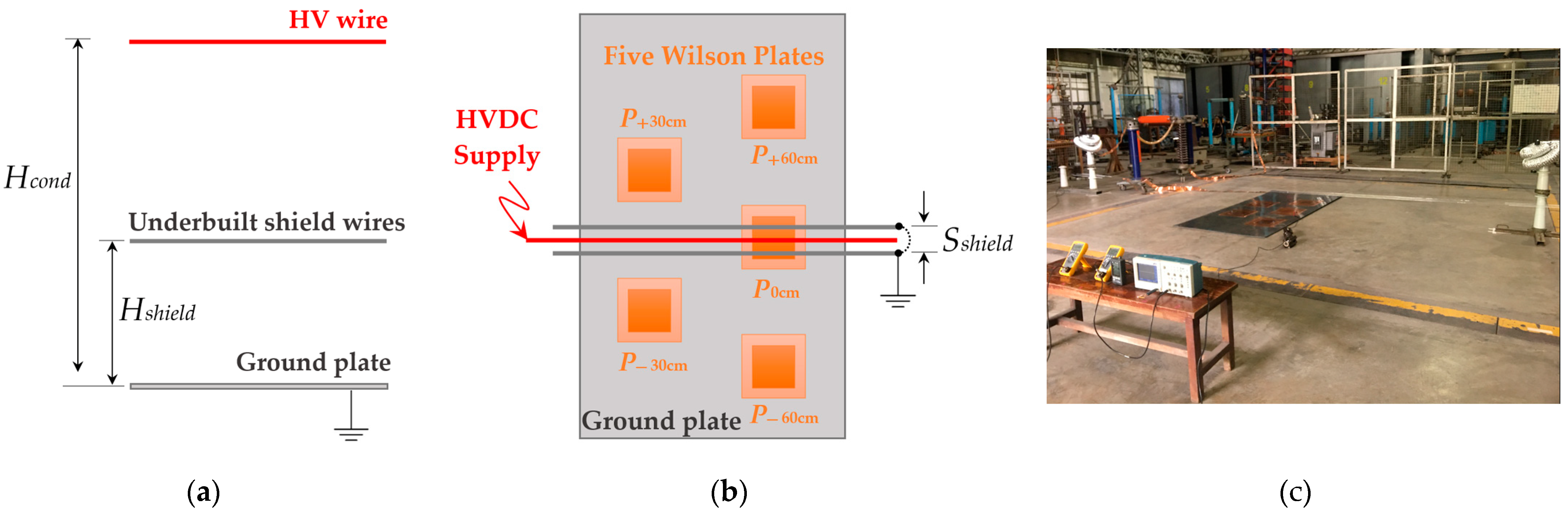
3. Configurations and Boundary Conditions

We carry out the numerical simulation for a reduced scale configuration and two full scale configurations, as shown in Figure 2. The figure shows 2D arrangements of the line and shielding conductors above ground. The reduced scale configuration in Figure 2a is used for comparison with our experimental results. The effect of underbuilt shield wires on the ion current density is observed. For the full-scale configurations, we treat the ±250 kV configuration in Figure 2b to study the wind effect on the bipolar lines and to make a comparison with reference [3]. Figure 2c shows the full-scale configuration of the ±500 kV double circuit lines. It presents the HVDC lines to be converted from existing HVAC ones. For the case with DMRC, the lowest bundled conductors are utilized to be the DMRC, which is the ground return path of the converted circuits. Since no current flows through the DMRC in the normal condition, we assume that the voltage on the conductors is zero.

Table 1. Geometrical parameters of the configurations.

Configurations	Line Voltage (kV)	${\mathit{H}}_{\mathit{cond}}$ (m)	${\mathit{r}}_{\mathit{cond}}$ (cm)	Number of Conductors
Reduced scale	+70	0.648	0.09	1
Full scale	±250	10	1.0	1
	±500	35 (circuit no.1) 24 (circuit no.2)	1.695	4

shows the geometrical parameters: the conductor height $H_{\mathit{cond}}$, the conductor radius $r_{\mathit{cond}}$ and the number of conductors of each pole. Note that the radius of shield wire and the DMRC are the same as the HV conductors. For Figure 2c, $S_{\mathit{bundle} }$= 45.7 cm, $S_{\mathit{pole}1 }$= 12.5 m, $S_{\mathit{pole}2 }$= 13 m, $S_{\mathit{DMRC} }$= 13.5 m and $H_{\mathit{DMRC} }$= 13 m. The parameters are referred from those of the existing AC lines.

For the calculation by the FVM, the open-air domain is truncated to a region of height $H_a$ and width W. A ground zone of depth $H_g$ and width W is added to treat the charge dissipation in the ground, as to be explained later. The domain of simulation is shown in Figure 3a. For 70 kV and ±250 kV configurations, $H_a$ and W are greater than 5 times and 10 times of the conductor height $H_{\mathit{Cond}}$, respectively, and $H_g$ is 3 times of $H_a$. We select $H_a$ = 100 m, W = 200 m and $H_g$ = 50 m for the ±500 kV configuration. Note that the height and the width of the simulation domain are sufficiently larger than those of the region of interest by 2 times and 10 times, respectively. The potential on the HV conductors is fixed to $+V_{\mathit{Cond}}$ or $-V_{\mathit{Cond}}$, depending on their polarity. The ground zone is set to zero potential. The fictitious boundaries of the air zone take the Neumann condition. For the wind conditions, we set the velocity inlet on the left air boundary and set the zero pressure outlet on the opposite side. Space charges are initiated and updated in each ionization zone of the HV conductors. We assume that the ion movement has no effect on the wind and all domains have the constant temperature of 27 °C.

4. Simulation

Quadratic meshes are utilized for all simulations shown in Figure 3b. The upwind FVM of ANSYS FLUENT software is used to solve the ion flow field. We define scalar variables ${\varphi }_k$ described by ${\varphi }_1=\frac{{\rho }_{+}\left(t\right)}{{\rho }_m}$, ${\varphi }_2=\frac{{\rho }_{-}\left(t\right)}{{\rho }_m}$, ${\varphi }_3=V\left(t\right)$ for the positive charges, negative charges and electric potential, respectively. The mass density ${\rho }_m$ = 1.225 kg/m³. ANSYS FLUENT solves the scalars based on a general transportation equation [15]

$$\frac{\partial {\rho }_m{\varphi }_k}{\partial t}+\nabla ·\left({\rho }_m{\mathbf{u}}_k{\varphi }_k - {\Gamma }_k\nabla \varphi k\right)=S_{\varphi k}$$

(10)

In Equation (10), the temporal change is related to the convection due to the flow velocity ${\mathbf{u}}_k$, the diffusion of coefficient ${\Gamma }_k$ and the source term $S_{\varphi k}$. The definitions of ${\varphi }_k$ ${\mathbf{u}}_k$, ${\Gamma }_k$ and $S_{\varphi k}$ for solving the transportation of ions and Poisson’s equation are given in

Table 2. Definition of ion flow field variables to Equation (10).

k	${\mathbf{u}}_{\mathit{k}}$	${\mathit{\Gamma }}_{\mathit{k}}$	${\mathit{S}}_{{\mathit{\varphi }}_{\mathit{k}}}$
1	${\mu }_{+}\mathbf{E}\left(t\right)+\mathbf{w}\left(t\right)$	${\rho }_m{D}_{+}$	$-R \frac{{\rho }_m^2{\rho }_{+}\left(t\right){\rho }_{-}\left(t\right)}{e}$
2	$-{\mu }_{-}\mathbf{E}\left(t\right)+\mathbf{w}\left(t\right)$	${\rho }_m{D}_{-}$	$-R \frac{{\rho }_m^2{\rho }_{+}\left(t\right){\rho }_{-}\left(t\right)}{e}$
3	N/A	${\mathit{\epsilon }}_{ 0}$	${\rho }_{+}\left(t\right) - {\rho }_{-}\left(t\right)$

. Three coupling equations are calculated by using quadratic elements. The turbulent flows are considered in our fluid simulation. Details of the calculation by the upwind FVM are referred to in reference [15].

4.1. Space Charge Initialization

The initial charge density ${\rho }_0$ occurs on the conductor surface, where $E>E_C$. The charge density in the ionization layer is initialized as [16]

$${\rho }_0 = \frac{E_g}{E_C} \frac{{8\epsilon }_{ 0}{V}_C \left(V_{\mathit{cond}}-{ V}_C\right)}{r_{\mathit{cond}}{ H}_{\mathit{cond}}{ V}_{\mathit{cond}} \left({5 - 4V}_C/V_{\mathit{cond}}\right)}$$

(11)

where $E_g$ is the ground-level electric field, $V_C$ is the corona-onset voltage and $V_{\mathit{cond}}$ is the conductor voltage magnitude. We update the charge density ${\rho }_{i+1}$ of the next time step i + 1 from the electric field $E_i$ and charge density ${\rho }_i$ at the current time step i as

$${\rho }_{i+1}={\rho }_i\left(1+\frac{E_i-E_C}{E_i+E_C}\right)$$

(12)

4.2. Ground Zone

The ions produced by the corona discharge dissipate in the ground (typically soil). For the simulation, we utilize a fictitious diffusion in the ground zone to reduce the charge aggregation without using additional source terms. The diffusion coefficient of the ground zone $D_g$ is taken as a multiplication of that in the air. We take $D_{g\pm } =$ 10⁶$D_{\pm }$ to obtain sufficiently fast dispersion of the ions in the ground [17].

4.3. Calculation Procedures

Figure 4 displays the calculation procedures. The steps can be explained as follows.

Initial values of $V\left(t\right)$ and $\mathbf{E}\left(t\right)$ are determined for each zone in Figure 3a, where ρ = 0 everywhere (i.e., in the space charge free condition).

• If $\mathbf{E}\left(t\right)$ on the conductor surface exceeds the corona-onset electric field in Equation (9), the initial charge density ${\rho }_0$ from Equation (11) is added to the ionization zone.
• Equation (10) is used to calculate the space charge transportation and the solution of Poisson’s equation.
• In the ionization zone, the charge density is updated using Equation (12).

Steps 3 and 4 are repeated until the electric field and the current density reach their stability at a small height above the ground plane. The convergence criterions terminate when the ground-level results vary between time steps by less than 0.01% for the electric field and 0.1% for the current density.

5. Experiments

Figure 5 shows the experimental setup. We carried out a reduced-scale experiment in the laboratory for comparison with the simulation results. Corona discharge was generated from a copper wire of 0.9 mm radius and 64.8 cm height. The wire was mounted on two supporting insulators and it was energized to 70 kV by an HVDC test system. The voltage was supplied from a test transformer and an HV rectifier. A resistive divider was used to measure the applied voltage. We installed underbuilt shield wires of 0.9 mm radius under the HV wire. Three values of the height $H_{\mathit{shield}}$ of the wires were used for the case with one shield wire. Three values of the spacing $S_{\mathit{shield}}$ between the wires were used for the case with two and three shield wires at the same 28 cm height. The underbuilt shield wires were grounded.

Five Wilson plates of 20 × 20 cm² were set above the ground plate for ion current measurement. The plates were placed at lateral distances of 0, ±30 and ±60 cm from the center line of the HV wire, as shown in Figure 5b. A 1 MΩ resistor was connected between each plate and the ground. The voltage across the resistor was measured to obtain the average ion current density $J_{\mathit{avg}}$ [18]. Before each measurement, the residual charges on the Wilson plates were discharged to the ground. A digital multimeter and an oscilloscope were used to measure the voltage across the resistor.

6. Results and Discussion

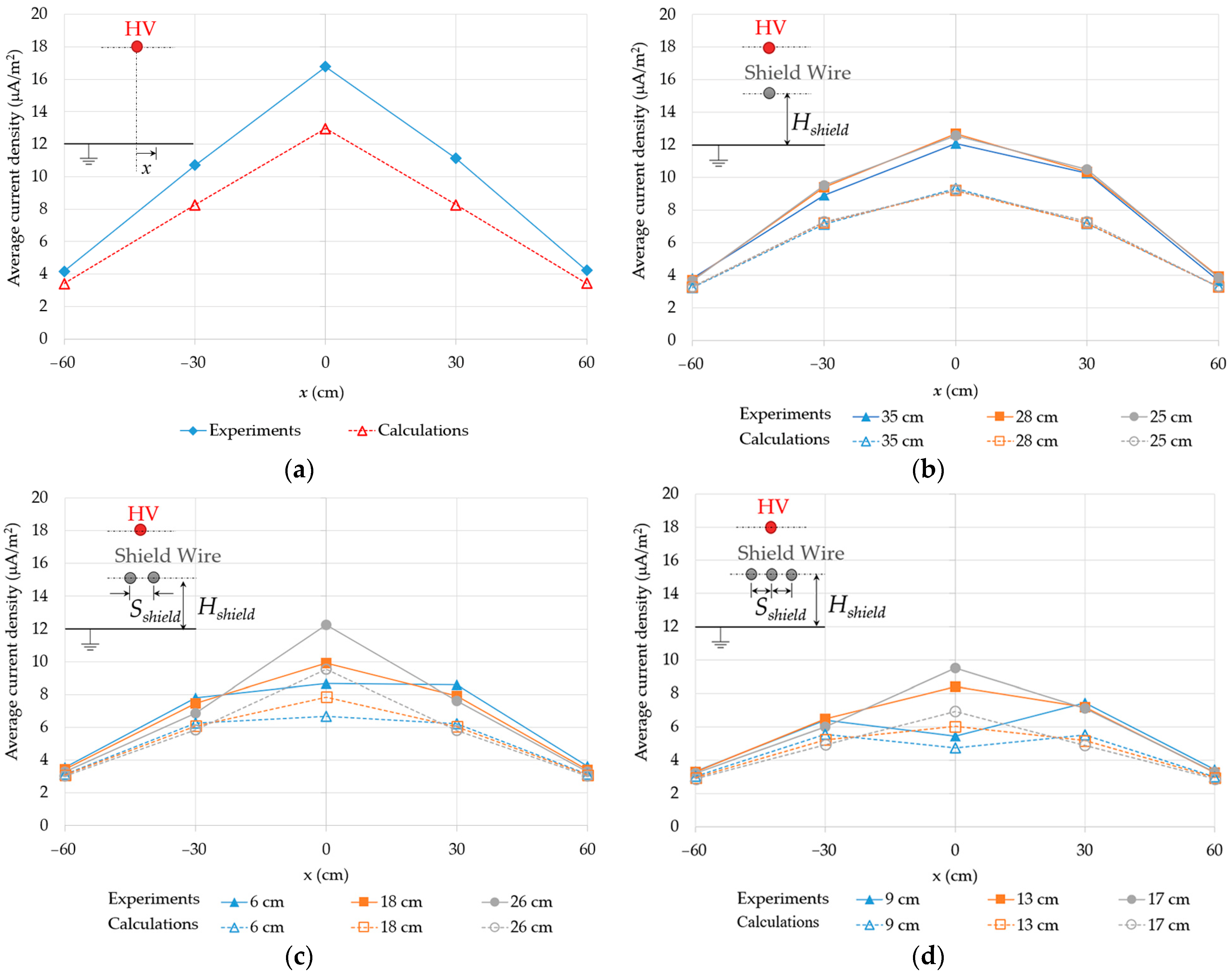
6.1. Reduced Scale Configuration

The number of meshes and elements varies between cases. Approximately 437,000 elements and 1,315,000 nodes are used. When the corona occurs, the transient process starts with ions generated near the conductor surface. The ions move to ground. The electric field in the gap between the conductor and the ground is modified. The ion current density is also adapted at the same time. The stability begins when the electric field is maintained on the corona onset value. The electric field and ion current density are evaluated at a small height of 1.8 cm above ground, where the values are stable in the steady state. The difference in Figure 6 compares the average current density $J_{\mathit{avg}}$ on the Wilson plates from the experiment with that from the calculation. The abscissa x is the lateral distance from the center line of the HV wire. For the case without the shield wire in Figure 6a, the experimental and calculated $J_{\mathit{avg}}$ have a similar tendency. The difference was 29% at x = 0 cm (right under the HV wire). For the case with one shield wire in Figure 6b, the tendency also agrees between the calculation and the experimental results. The height $H_{\mathit{shield}}$ does not have a clear impact on the $J_{\mathit{avg}}$. For the case with two shield wires where $H_{\mathit{shield}}$ = 28 cm in Figure 6c, both the calculation and the measurement show a flat distribution of $J_{\mathit{avg}}$ between x = −30 and 30 cm for $S_{\mathit{shield}}$ = 6 cm. The peak $J_{\mathit{avg}}$ occurs x = 0, with increasing $S_{\mathit{shield}}$ to 18 or 26 cm. For the case with three shield wires ($H_{\mathit{shield}}$ = 28 cm) in Figure 6d, the spacing $S_{\mathit{shield}}$ = 9 cm yields two peaks $J_{\mathit{avg}}$ at x = ±30 cm. For $S_{\mathit{shield}}$ = 13 and 17 cm, the $J_{\mathit{avg}}$ peak is under the HV wire (x = 0).

In summary, the simulated current distribution shows similar tendency to the measured profiles. The measured current density is higher than the calculated one approximately 15 to 40%. The discrepancy may be caused by the size of the Wilson plates, the flatness of the ground plate or the surface condition of the corona wire. The deviations of all experiments are ±0.8 μA/m² for x = ±60 cm, ±1.2 μA/m² for x = 30 cm and ±1.4 μA/m² for x = 0 cm that is highest under the HV wire. One underbuilt shield wire reduces the peak $J_{\mathit{avg}}$ under the HV wire by more than 25% when compared with the case without the shield wire. Increasing the number of shield wires with the suitable spaces can reduce $J_{\mathit{avg}}$ under the HV wire by more than 50%, as the case with three shield wires where $H_{\mathit{shield}}$ = 28 cm and $S_{\mathit{shield}}$ = 9 cm in the current work.

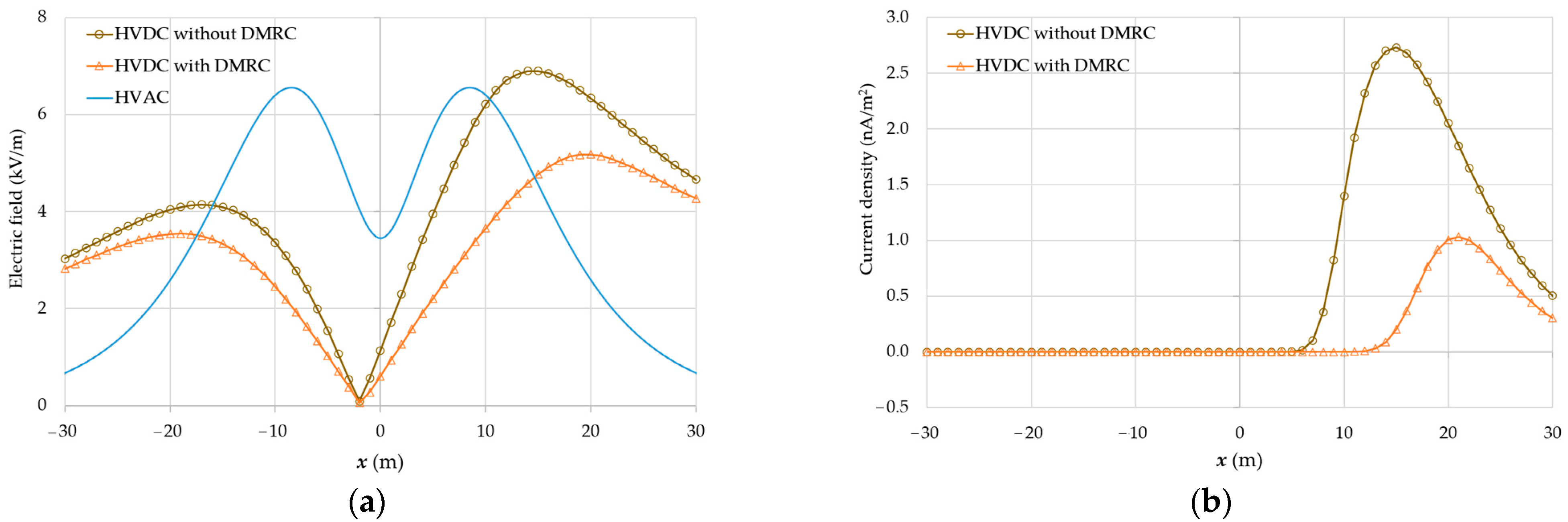
6.2. Full Scale Configuration of ±250 kV Lines

For comparison with the results in reference [3], the following parameters are used. The pole spacing $S_{\mathit{pole}}$ (see Figure 2b) is 10 m. $E_C$ is set to 27.3 kV/cm, μ is 1.5 × 10⁻⁴ m²/(Vs) and D is 3.88 × 10⁻⁶ m²/s for both positive and negative ions. Approximately 146,000 elements and 441,000 nodes are used for the simulated models. The calculation is performed for a case without wind and with wind flowing from the negative to positive conductors. The wind profile is applied with $w_r$ = 0.5 m/s and α = 0.3 according to the reference. Figure 7 shows the calculated profiles of the ground electric field $E_g$ and the ion current density $J_g$ from the calculation. Note that we take the horizontal distance x from the center line to be positive in the direction to the conductor of positive polarity. For the case without wind, the distribution of $E_g$ and $J_g$ agree well with those in the reference, although discrepancy occurs farther from the HV lines ($\left|x\right|$ > 10 m). Under the wind condition, $E_g$ and $J_g$ decrease on the upwind side and increase on the downwind side, which is consistent with the reference. The positions at the peak of $E_g$ and $J_g$ are displaced approximately 1.5 m from that in the absence of wind, whereas the displacement is not clear in reference [3]. The peak magnitudes with and without the wind differ from those in the reference about −1% to −7% for $E_g$ and −6% to +16% for $J_g$.

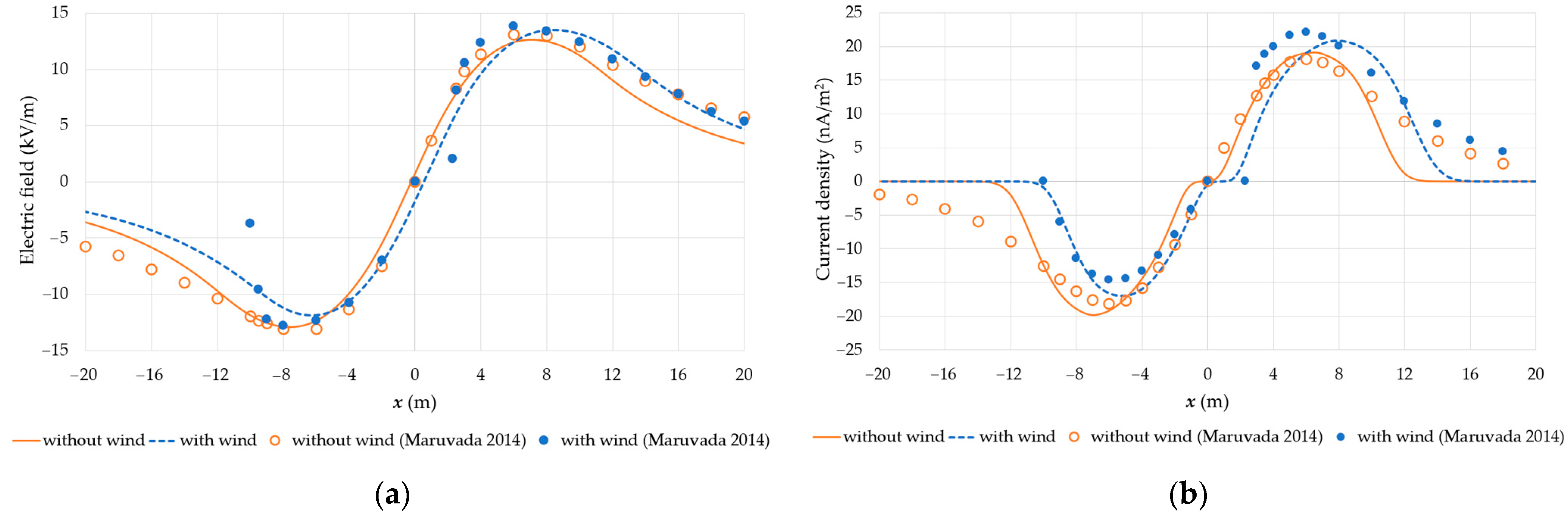
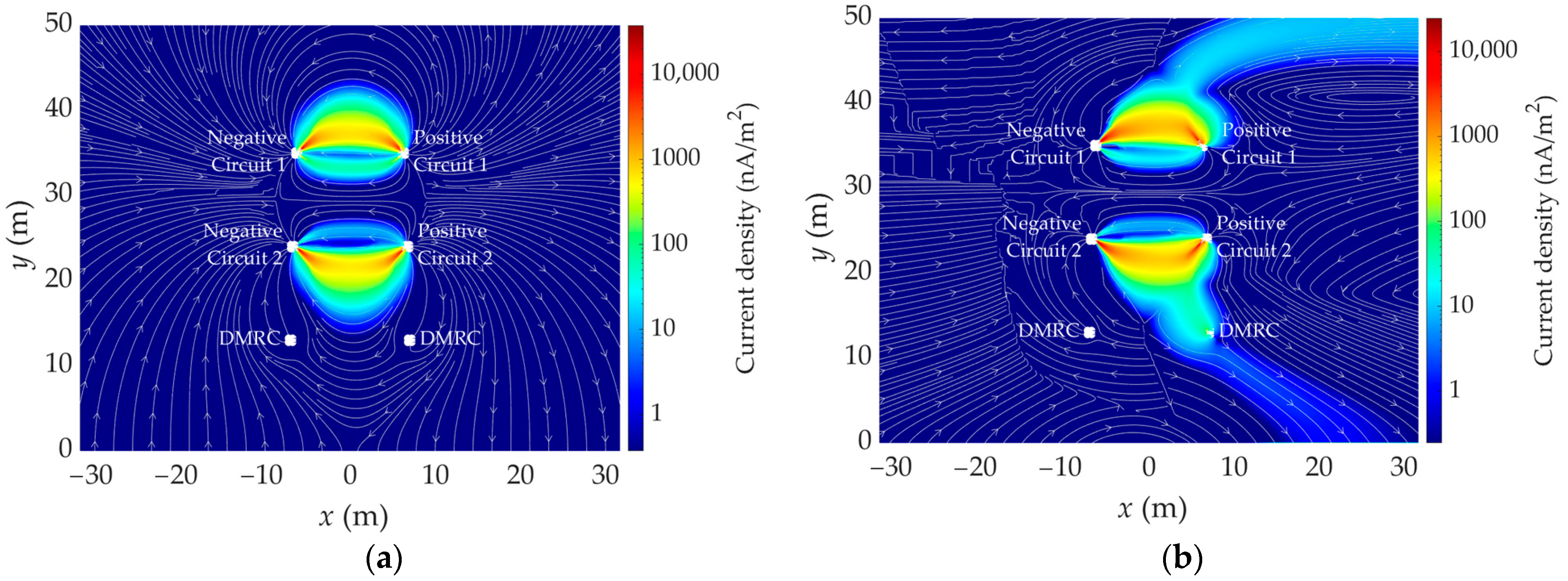
6.3. 500. kV Full-Scale Configuration

6.3.1. In the Absence of Wind

We consider the configuration in Figure 2c without and with DMRC, respectively. For the simulation, around 406,000 elements and 1,114,000 nodes were used. The values of ion mobility and diffusion coefficient are as follows ${\mu }_{+}$ = 1.4 × 10⁻⁴ m²/(Vs), ${\mu }_{-}$ = 1.8 × 10⁻⁴ m²/(Vs), $D_{+}$ = 3.62 × 10⁻⁶ m²/s and $D_{-}$ = 4.65 × 10⁻⁶ m²/s [15]. Figure 8 shows the electric field and ion current density at the ground level under the no-wind condition. We also give the electric field in the case of the 500 kV HVAC energization for comparison. Without DMRC, the peak of $E_g$ is lower than that of the HVAC lines by 33%. The peak positions are at x = ±16 m, i.e., they are farther from the center than those of the HVAC lines, resulting in higher $E_g$ near the edge of ROW. With DMRC, $E_g$ is reduced, i.e., the DMRC functions similarly to the shield wires, as explained in Section 6.1. The peak $E_g$ is reduced approximately by 17% from the peak without DMRC. The peak positions are x = ±19 m, slightly farther from the center line.

The ion current density profiles exhibit an unsymmetrical distribution with respect to x = 0. They are caused by different values of μ and D between the negative and positive ions. The peaks at center line and at the edge of ROW can be seen in Figure 8b. The highest magnitude is near the edge of ROW on the negative polarity side. The magnitudes of the other local peaks are much smaller. For the ±500 kV HVDC configurations, the distributions of $J_g$ are considerably different from the results of the ±250 kV lines in Figure 7b. $J_g$ is very small in Figure 8b because the separation $S_{\mathit{pole}}$ between the positive and negative lines is much smaller than the distance $H_{\mathit{cond} }$ to the ground. Figure 9 shows the ion current density distribution with its flowing direction for the case with DMRC. We can see from Figure 9a that almost all ions migrate between the line conductors in the absence of wind. The maximum magnitude of $J_g$ is 0.0036 nA/m² without DMRC and is reduced to 0.0029 nA/m² with the DMRC. That is, the DMRC reduces $J_g$ by 19% in the absence of wind.

6.3.2. In the Presence of Wind

The steady wind velocity model described in Section 2.2 is applied with the annually average wind data, $w_r$ = 1.3 m/s and α = 0.4. The wind direction is from the negative to the positive conductors, as $E_g$ and $J_g$ peaks are higher [1]. Figure 10a compares $E_g$ of both configurations under the wind condition. The electric field in the figure is unsymmetrically distributed in the presence of the wind. $E_g$ decreases by 0.4 kV/m on the upwind side (negative voltage) and increases by 2.7 kV/m on the downwind side (positive voltage). As a result, $E_g$ peaks on the upwind and downwind sides are approximately −9% and 63% of those in the no-wind condition, respectively. Note that the $E_g$ peak on the downwind side is higher than the peak of the HVAC lines. The positions of the $E_g$ peaks are shifted slightly by the wind condition. At the edge of ROW on the downwind side, the field is also significantly higher than that of the HVAC lines (by 6.9 times). Figure 9a shows that the DMRC considerably mitigates $E_g$. The peak positions change to x = −19 and 20 m, i.e., they are shifted farther from the center line (x = 0). At the edge of ROW on the downwind side, the migration of $E_g$ by DMRC is mild. In conclusion, we have found that the wind increases $E_g$ significantly on the downwind side and using DMRC can reduce the peak of $E_g$ magnitude by 25% under the wind condition.

In Figure 9b, the wind also strongly affects the current density distribution. The current distribution shifts to the downwind and has some ion terminating at the ground. Figure 10b shows $J_g$ in the presence of the wind. It is worth noting that the negative ion current is suppressed, resulting in the predominant positive current on the ground. Compared with Figure 8b, the peak of $J_g$ increases significantly to 2.73 nA/m² for the HVDC lines without DMRC. The position of peak is x = 15 m, the same as that of $E_g$ peak. With DMRC, $J_g$ has a smaller peak value of 1.01 nA/m² at x = 20 m. The maximum of $J_g$ is still located within the ROW, but quite close to the ROW corridor. The DMRC reduces the $J_g$ maximum to be 63% of the case without DMRC in the presence of wind.

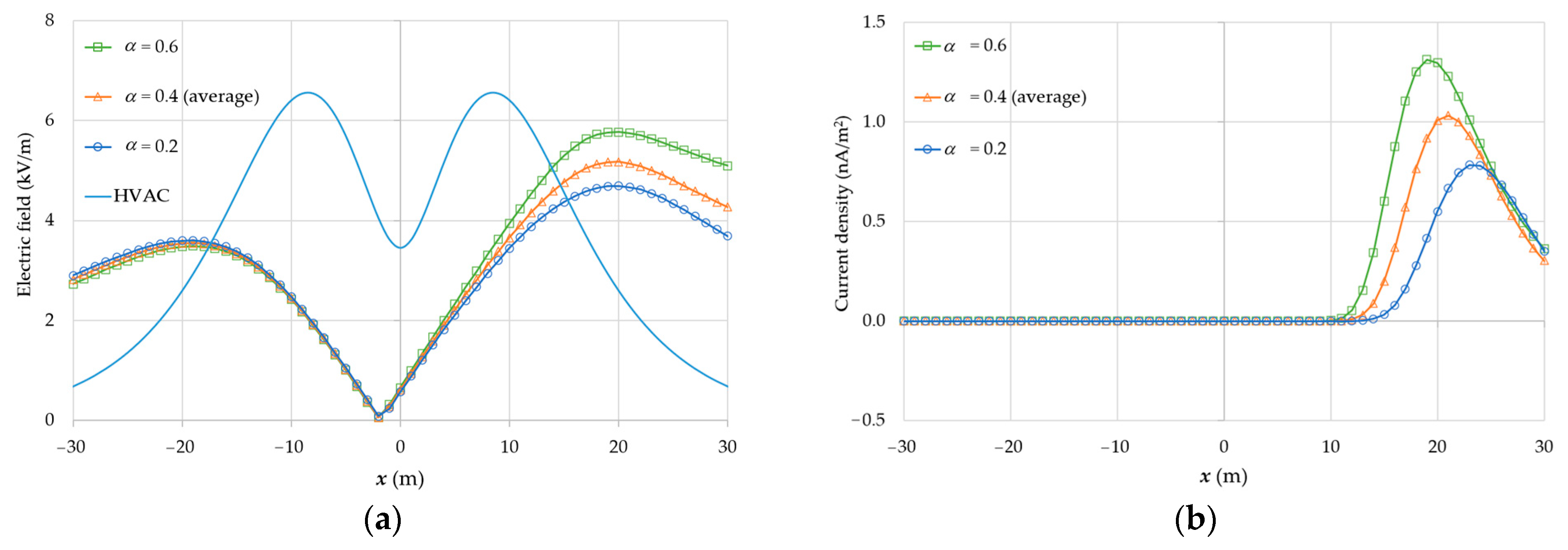
6.3.3. Variation with Wind Parameters

The configuration with DMRC is selected for the simulation with different wind parameters. Figure 1 implies a wide range of wind velocity that can occur practically. Therefore, we perform the simulation for the ±500 kV lines with maximal and minimal wind shear coefficients (α = 0.2 and 0.6). Figure 11a shows $E_g$ under the wind condition for different α. From the figure, $E_g$ obviously changes on the downwind side. The peaks are higher with increasing α. However, with α = 0.6, the peak of $E_g$, increased by 11%, is still lower than that of the HVAC lines. The position of the peak hardly changes with α. At the edge of the ROW, the downwind side $E_g$ is also higher with larger α.

Figure 11b shows the variation of $J_g$ with α. Similar to the $E_g$ distribution, $J_g$ varies clearly with α only on the downwind side. The $J_g$ peak value increases with α. Increasing α from the annual average 0.4 to 0.6 results in higher $J_g$ peak by 30%. With larger α, stronger wind takes place at the conductor, thus moving more ions to the downwind side of the conductors. The electric field and the charge density are then enhanced on the downside, leading to the larger $J_g$ on the ground. The positions of peak $J_g$ for α = 0.2 and 0.6 are slightly deviated from that of α = 0.4.

7. Conclusions

The ion flow field of the three HVDC line configurations have been studied. For the monopolar configuration with underbuilt shield wires, the calculation results show good agreement of the distribution of $E_g$ and $J_g$ with the measurement results. For the ±250 kV bipolar configuration, the ground-level electric field $E_g$ and the current density $J_g$ agree with the results in reference to some discrepancy at a distance farther than 10 m from the lines. The ±500 kV HVDC configurations are analyzed to study the wind effects on $E_g$ and $J_g$ for the cases without and with DMRC. In the absence of wind, $E_g$ has its peak magnitude lower than that of the HVAC lines, but it is higher at the ROW edge. $J_g$ is very low on the ground. Our results show the significant role of the wind as the magnitudes of $E_g$ and $J_g$ on the downwind side significantly increase. Without DMRC, the peak of $E_g$ is higher than that of the HVAC lines. The increase of the wind shear factor α also magnifies $E_g$ and $J_g$ by 11% and 30%, respectively. Our results can clarify that the use of the DMRC effectively mitigates $E_g$ and $J_g$ in all wind cases, although a high electric field still occurs at the edge of ROW. As the conductor temperature and surrounding air may change during the HVDC line operation, its effect is subjected to a study in the future.

References

1. Hara, M.; Hayashi, N.; Shiotsuki, K.; Akazaki, M. Influence of wind and conductor potential on distributions of electric field and ion current density at ground level in DC high voltage line to plane geometry. IEEE Trans. Power Appar. Syst. 1982, PAS-101, 803–814. [Google Scholar] [CrossRef]
2. Takuma, T.; Kawamoto, T. A very stable calculation method for ion flow field of HVDC transmission lines. IEEE. Trans. Power Deliv. 1987, 2, 189–198. [Google Scholar] [CrossRef]
3. Maruvada, P.S. Influence of Wind on the Electric Field and Ion Current Environment of HVDC Transmission Lines. IEEE. Trans. Power Deliv. 2014, 29, 2561–2569. [Google Scholar] [CrossRef]
4. Yi, Y.; Zhang, C.; Wang, L.; Chen, Z. Statistical evaluation and numerical analysis of effect of transverse wind on ionized field of ±800 kV UHVDC operating transmission lines. Electr. Power Syst. Res. 2016, 140, 560–567. [Google Scholar] [CrossRef]
5. Yi, Y.; Chen, Z.; Tang, W.; Wang, L. Predictive calculation of ion current environment of dc transmission line based on ionised flow model of embedded short-term wind speed. IET Gener. Transm. Distrib. 2018, 12, 3837–3843. [Google Scholar] [CrossRef]
6. Yi, Y.; Wang, L.; Chen, Z. Estimating the environmental impacts of HVDC and UHVDC lines for large-scale wind power transmission considering height-dependent wind and atmospheric stability. Int. J. Electr. Power Energy Syst. 2022, 138, 107868. [Google Scholar] [CrossRef]
7. Yin, H.; Zhang, B.; He, J.; Wang, W. Restriction of ion-flow field under HVDC transmission line by installing shield wire. IEEE. Trans. Power Deliv. 2013, 28, 1890–1898. [Google Scholar] [CrossRef]
8. Tian, F.; Zhanqing, Y.; Zeng, R.; Yin, H.; Zhang, B.; Liu, L.; Li, M.; Li, R.; He, J. Resultant electric field reduction with shielding wires under bipolar HVDC transmission lines. IEEE. Trans. Magn. 2014, 50, 221–224. [Google Scholar] [CrossRef]
9. Noosuk, A.; Mermork, T.; Semjan, A.; Rahman, M.S.; Dawood, A.R.; Ismail, S.B.; Kurth, R.D.; Atmuri, S.R. Commissioning experience of the 300 MW Thailand-Malaysia interconnection project. In Proceedings of the IEEE/PES Transmission and Distribution Conference and Exhibition, Yokohama, Japan, 6–10 October 2002; Volume 2, pp. 1004–1009. [Google Scholar]
10. CIGRE Working Group B2. 41. Guide to the Conversion of Existing AC Lines to DC Operation; Technical Brochure No. 583; CIGRE-International Council on Large Electric Systems: Paris, France, 2014; pp. 8–19. [Google Scholar]
11. Lattarulo, F.; Amoruso, V. Filamentary Ion Flow: Theory and Experiments, 1st ed.; Wiley-IEEE Press: Hoboken, NJ, USA, 2014; pp. 25–61. [Google Scholar]
12. Manwell, J.F.; McGowan, J.G.; Rogers, A.L. Wind Energy Explained: Theory, Design and Application, 2nd ed.; John Wiley & Sons: Chichester, UK, 2010; pp. 43–52. [Google Scholar]
13. Mega, O.; Kasemsan, M.; Thayukorn, P. Wind Shear Coefficient at 23 Wind Monitoring Towers in Thailand. J. Sustain. Energy Environ. 2015, 6, 61–66. [Google Scholar]
14. Maruvada, P.S. Corona Performance of High-Voltage Transmission Lines, 1st ed.; Research Studies Press Ltd.: Baldock, UK, 2000; pp. 82–86. [Google Scholar]
15. Versteeg, H.; Malalasekera, W. An Introduction to Computational Fluid Dynamics: The Finite Volume Method, 2nd ed.; Pearson Education Limited: Harlow, UK, 2007; pp. 1–39. [Google Scholar]
16. Yin, H.; He, J.; Zhang, B.; Zeng, R. Finite Volume-Based Approach for the Hybrid Ion-Flow Field of UHVAC and UHVDC Transmission Lines in Parallel. IEEE. Trans. Power Deliv. 2011, 26, 2809–2820. [Google Scholar] [CrossRef]
17. Choopum, C.; Techaumnat, B. Investigation of the Effects of Ion Diffusivity on the Ion Flow Field Simulation. In Proceedings of the 19th Electrical Engineering/Electronics, Computer, Telecommunications and Information Technology (ECTI-CON), Prachuap Khiri Khan, Thailand, 24–27 May 2022; pp. 1–5. [Google Scholar]
18. Fang, C.; Cui, X.; Zhou, X.; Lu, T.; Zhen, Y.; Li, X. Impact Factors in Measurements of Ion-Current Density Produced by High-Voltage DC Wire’s Corona. IEEE. Trans. Power Deliv. 2013, 28, 1414–1422. [Google Scholar] [CrossRef]
Figure 1. The 24-h wind profile information used for the study.
Energies 16 00198 g001
Figure 2. Configurations of calculation: (a) +70 kV reduced scale; (b) ±250 kV full scale; (c) ±500 kV full scale.
Energies 16 00198 g002
Figure 3. Calculation domain: (a) zones and boundary conditions; (b) meshing.
Energies 16 00198 g003
Figure 4. Flow chart of the simulation.
Energies 16 00198 g004
Figure 5. Experimental setup of the reduced-scale configuration: (a) side view; (b) top view; (c) photo of experimental setup.
Energies 16 00198 g005
Figure 6. Comparison between the experimental and calculated average current density of the reduced scale configuration: (a) no shield wire; (b) one shield wire at H shield = 25, 28 and 35 cm; (c) two shield wires at S shield = 6, 18 and 26 cm; (d) three shield wires at S shield = 9, 13 and 17 cm.
Energies 16 00198 g006
Figure 7. Electric field and ion current density at the ground level of the ±250 kV configuration: (a) electric field E g ; (b) ion current density J g .
Energies 16 00198 g007
Figure 8. Electric field magnitude and ion current density at the ground-level of the ±500 kV configuration with and without DMRC under the no wind condition: (a) electric field magnitude; (b) ion current density.
Energies 16 00198 g008
Figure 9. Ion current density distribution of the ±500 kV configuration with DMRC: (a) in the absence of wind; (b) in the presence of wind with average α.
Energies 16 00198 g009
Figure 10. Electric field magnitude and ion current density at the ground level of the ±500 kV configuration under the annually average wind condition: (a) electric field magnitude; (b) ion current density.
Energies 16 00198 g010
Figure 11. Variation of electric field and ion current density with the wind shear coefficient for the ±500 kV HVDC configuration: (a) electric field magnitude; (b) ion current density.
Energies 16 00198 g011