Abstract
This paper presents the development and use of benchmarking grey-box models for the detection and diagnosis of multiple-dependent faults (MDFDD) of a water-cooled centrifugal chiller. Models are developed using data recorded by a Building Automation System (BAS) from a central cooling plant of an institutional building. The forward residual-based fault detection model identifies a fault symptom, when the difference between the measured value of target variable and benchmarking value exceeds the corresponding threshold. For the fault diagnosis, most publications start from a known single fault and establish the impact on following variables in the system. This paper presents a rule-based backward approach. The proposed method identifies if (i) the fault symptom is correct (i.e., a variable has abnormal values), or (ii) the fault symptom is incorrect (i.e., the symptom of target variable is caused by impacts generated by other faulty variables due to the dependency between variables), or (iii) both target and regressor variables are abnormal. For testing the proposed MDFDD model, some artificial faults are inserted into the measurement data file, and results are discussed about the method potential for the application.
1. Introduction
In Canada, the energy used for buildings reached to 2.79 EJ in 2018, accounting for 28.78% of overall energy usage [1]. The heating, ventilation, and air conditioning (HVAC) systems use about 70% of building electricity [2] or 50% of energy consumption for non-domestic buildings [3]. Faults of HVAC systems lead to energy waste [4], increase in maintenance cost [5] and the degradation or even possible damages to HVAC equipment [6,7]. For instance, a study about the building maintenance reported 11 fault cases of chillers and boilers every year per 1000 m2 floor area [8].
As modern HVAC systems become increasingly complex, the combined effect of different faults of such systems leads to increase difficulties for the detection and isolation [9]. Building automation systems, installed in large commercial and institutional buildings, are gold mines of data about the operation and performance of HVAC systems. The maintaining HVAC systems at optimum operation status becomes one of the most important approaches for improving energy efficiency [10]. Some questions that should be investigated with respect to HVAC systems are listed below:
(1) Could the diversity and quality of data stored in BAS be considered sufficient for the detection and diagnosis of faults.
(2) How cost-effective is the development and use of FDD models based on data from BAS, compared with models based on dedicated monitoring systems.
(3) How can dependent faults be detected using data at 10–15 min time steps.
(4) How might the uncertainty of measurements affect the fault detection.
(5) What is the minimum number and type of sensors for each potential fault that should be used.
(6) What is the potential of virtual sensors for FDD, when considering the cost and uncertainty of prediction.
2. Literature Review
A fault is defined as a departure from an acceptable range of observed variable or calculated parameter associated with the equipment [11]. Due to impacts caused by faults in HVAC systems, a number of research studies have focused on fault detection and diagnosis (FDD) methods. An early study of components failure of a household refrigerator was published in 1988 [12].
Most publications have discussed the detection and diagnosis of single faults [9,13] in vapor compression chillers, HVAC systems [14,15,16], and air handling units (AHU) [17]. Data-driven FDD methods are commonly developed with black-box FDD techniques because of simplicity. Rule-based FDD is the second most common FDD method. A single fault is usually much simpler to deal with, compared with the multiple simultaneous faults (MSFs) that occur at the same time but at different locations [9,18]. The simultaneous or sequential faults can be classified in four categories [19]: (i) induced faults, (ii) independent multiple faults, (iii) masked multiple faults, and (iv) dependent multiple faults.
The detection and diagnosis of multiple/simultaneous faults in HVAC systems is still a challenge, since the combination of several faults makes difficult the separation of individual faults.
Multiple faults (MFs) and multiple dependent faults (MDFs) are two related but distinct topics. Both refer to multiple faults, but differ in whether dependency among faults exists. A fault symptom might not reveal a real fault, but could be the result of another fault in the system.
Some publications ignore the dependency of multi-faults. Such methods cannot be used for the detection and diagnosis of multiple dependent faults. For example, ref. [20] assumed the case when independent faults occur simultaneously in two separate loops of a variable air volume (VAV) system: (i) the sensor of supply air temperature control loop, and (ii) the sensor of outdoor air control loop. Reference [21] proposed a set of 26 rules for the isolation of multiple single faults of air handling units. For instance, faults of mixed air temperature, chilled water circulating pump, and cooling coil valve controller can be detected. However, the interaction between the individual fault is not analyzed. As a result, the methods proposed in these two papers are not applicable to the detection and diagnosis of multiple dependent faults (MDFDD) in HVAC systems.
Only a small number of publications deal with methods for MDFDD in HVAC systems. Most studies started by inserting either (i) a physical fault in an experimental set-up, or (ii) a numerical abnormal value in the experiment data file or in the computer simulation results. The impact of such an artificial fault of the regressor variable was assessed on other subsequent variables (called target variables) by measurement or simulation. This approach has an important value on the understanding of the relationship between the cause (the fault) and the effect on other variables of subsequent equipment. A few examples are presented in this section.
Breuker and Braun [22] used measurements from a three-ton packaged rooftop unit along with polynomial models to develop a statistical, rule-based classifier of faults. Such rules show whether a particular measurement increases or decreases in response to a particular fault at steady-state conditions. For instance, the compressor valve leakage generally increases the discharge refrigerant temperature (Tdis) from the compressor above the normal value under steady-state condition. If measurements in a real rooftop units show the increase in Tdis, the detection rule indicates that the fault is caused by the compressor valve leakage; all other possible causes being neglected.
References [23,24,25] proposed one decoupling-based method to indicate the relationship between target variable and potential source of fault. They used an air-cooled roof top unit of three tons of refrigeration installed in a laboratory-controlled environment as a case study. Based on the theoretical analysis of physical processes in the system and within each equipment (e.g., compressor, condenser), and from experimental measurements, they proposed a decoupling-based method. The decoupling-based method simplifies the diagnosis by assuming that abnormal target variable (e.g., the discharge refrigerant temperature Tdis) is caused exclusively by one regressor variable, while the role of all other possible regressor variables is neglected. For instance, they concluded that the abnormal deviation of Tdis is only caused by the compressor valve leakage. The situation of faulty target variable (e.g, faulty sensor of Tdis) was not considered.
Kim and Braun [26] expanded previous work on FDD methods [23,24,25], and developed a MDFDD system that decouples the impacts of individual faults to estimate multiple faults that occur simultaneously. They developed virtual sensors for the compressor, expansion valve, condenser, evaporator, and refrigerant charge, using measurements from a four-ton rooftop unit in a laboratory-controlled environment, and the compressor map. When two simultaneous faults occur (e.g., the reduction in airflow rate due to condenser fouling, and compressor valve leakage) the impact ratio of each fault on the system performance (e.g., COP) degradation is isolated.
One can conclude that methods presented by [22,23,24,25,26] are forward methods, which detect the impact of some faults (e.g., compressor valve leakage) on the next sensors or equipment performance (e.g., chiller COP). These methods could be used as reference rules for the reverse detection of single faults. However, such rules can be applied directly only to the type of rooftop unit used in laboratory-controlled experiments. The level of detailed measurements of all variables used in laboratory work is not feasible for an HVAC equipment in existing buildings. Additional research is needed for the generalization of decoupling-based method to other configurations of HVAC systems and equipment.
This paper presents an alternative method for the detection and diagnosis of multiple-dependent faults (MDFDD) of water-cooled centrifugal chillers, using the measurement data from Building Automation System (BAS) of an institutional building. For this purpose, benchmarking grey-box models are developed as forward models for the detection of a fault symptom, when the difference between measurements and predictions of target variable exceeds a threshold value. Once the fault symptom is detected, rule-based backward fault diagnosis models are applied. The proposed method can be generalized by updating the model parameters with measurements from other chillers. Such an alternative method can be integrated in BAS for continuous commissioning of HVAC equipment.
This paper contributes to the research efforts for the detection of multiple dependent faults of a water-cooled centrifugal chiller, using data recorded by a Building Automation System (BAS). This topic is rarely discussed in the field of FDD for the HVAC systems. A forward residual-based fault detection approach and a rule-based backward approach are developed.
The paper is organized as follows: Section 3 presents the development of MDFDD method including the development of benchmarking models, detection of symptoms, and diagnosis of faults. Section 4 presents the case study and the model training and testing results for benchmarking grey-box models. Since there are no faults recorded during the chiller operation, numerical artificial faults are inserted in the measurement data file. Section 5 presents the results of MDFDD method under artificial faults. Section 6 presents conclusions and future work.
3. Method
The proposed MDFDD method is summarized as follows:
- (a)
- Key target variables that give essential information about the chiller performance are selected (e.g., the electric power input to the compressor, and chiller COP).
- (b)
- Benchmarking grey-box models that predict the expected operation values of selected target variables, under normal operation conditions, are developed using measurement data from building automation system (BAS). These models use measurements from regressor variables (e.g., the chilled water leaving temperature) that could be the source of abnormal performance of target variables.
- (c)
- If the residual of measured target value and predicted value exceeds the threshold, the fault symptom of target variable is detected.
- (d)
- A fault symptom might not reveal a real fault but could be the result of abnormal values of regressors (e.g., chilled water temperature), which are in the loop prior to the target variable. Thus, the target variable could be dependent of regressors. The backward fault diagnosis method looks for the diagnosis of regressors faults. Moreover, the faulty target variable itself can also generate the fault symptom.
- (e)
- The multiple-dependent fault detection and diagnosis (MDFDD) method concludes with three possible outcomes: (i) the target variable is faulty, (ii) the regressor variables are faulty, and (iii) both target and regressor variables are faulty.
3.1. Benchmarking Models
Three target variables are selected, as being potentially faulty, as examples for the development and application of proposed MDFDD method: the electric power input to the chiller (E), the coefficient of performance of the chiller (COP), and the condenser-water leaving temperature (Tcdwl). The grey-box model has several advantages: (1) robust [27], (2) requires less data and being fast to train [13], (3) extrapolates well to operating conditions outside the range of training dataset [27]. Thus, benchmarking grey-box models are selected to predict the three target variables.
The benchmarking models are developed from measurements of normal operation, i.e., without known problems. Regressors of benchmarking models are selected from available variables from BAS (Table 1 and Table 2) that show potential impact over the target variables. The benchmarking grey-box models present in an explicit format the potential impact of corresponding regressors. The method can be expanded to other target variables, if needed.
Benchmarking model of the electric power input to the chiller
Benchmarking model of the coefficient of performance (COP)
Benchmarking model of the condenser-water leaving temperature
where α, β, and γ with subscripts are the parameters to be identified during the training phase. is mean value of Tchwl over training dataset, as the information of Tchwl setpoint is unavailable from the case study. PLR is the part load ratio, defined as the ratio of evaporator cooling load at each time step (Qev,m, see Equation (10)) to the evaporator cooling load at design condition (Qev,des). mev,ref is the derived refrigerant mass flow rate at the evaporator (Equation (12)).
The following performance metrics are used to evaluate benchmarking grey-box models (Equations (4)–(8)):
where yi is the measured value, is the predicted value, is the mean value of measurements, is the covariance of y and , and σ is the standard deviation.
3.2. Forward Fault Detection Model and Evaluation
3.2.1. Forward Residual-Based Detection of Multiple-Dependent Faults
A fault symptom is detected when the residual is greater than the corresponding threshold. The following four fault symptoms are considered in this paper.
(a) A fault symptom is detected for the chilled water leaving temperature, if the following condition holds:
(b) A fault symptom is detected for the electric power input, if the following condition holds:
(c) A fault symptom is detected for the derived measurement of COP, if the following condition holds:
(d) A fault symptom of refrigerant flow rate (mev,ref) at the evaporator is detected, if the following condition holds:
Within this paper, a fault symptom only indicates the possibility of a real fault, and thus it requires the fault diagnosis. A question naturally comes up: when a fault symptom is detected, is the target variable faulty or regressor variable faulty or both are faulty? To respond this question, the backward fault diagnosis model is presented in Section 3.3.
3.2.2. Evaluation of Forward Fault Detection Model
The application of forward fault detection model returns a binary result: whether a condition is normal or faulty. Thus, to differentiate a fault from a normal condition of a variable is a classification problem. As illustrated by Figure 1, there are four classes of results (points): true positive (TP), false positive (FP), false negative (FN), and true negative (TN). TP and FN show the points when a system operates with a fault. Here, TP indicates the points above a threshold, and FN indicates the points below a threshold. TN and FP show the situation when a system operates with fault-free status; TN indicates the points below a threshold, and FP indicates the points above a threshold.
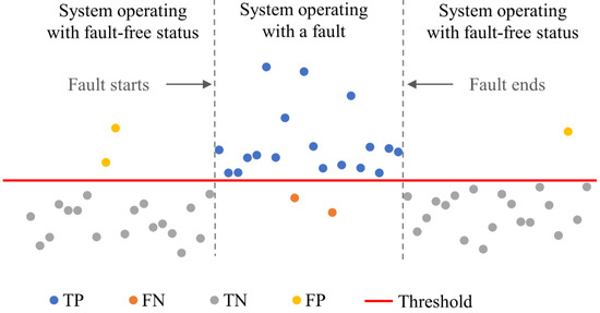
Figure 1.
Four classifications of points used for fault detection.
Three metrics are usually applied to evaluate fault detection models [28,29]: accuracy (AC) (Equation (13)), hit rate (HR) (Equation (14)), and false alarm rate (FAR) (Equation (15)), which corresponds to accuracy, precision, and sensitivity in the confusion matrix [30]. AC is defined as the percentage of points that are correctly classified by the model over the whole testing dataset, during both faulty time and fault-free time. HR is defined as the percentage of fault points that are successfully detected when a system is operating with a fault during only faulty time. FAR indicates the percentage of points that are misclassified during only fault-free time. Therefore, the three metrics cover all the time intervals over the test dataset. AC gives an overall view of the model, HR focuses on the intervals when faults are injected to a system, and FAR considers the time when a system operates under fault-free condition.
3.3. Backward Rule-Based Diagnosis of Multiple-Dependent Faults
Diagnosis of such faults is a more difficult task than the detection of single faults. This paper proposes a rule-based backward approach to diagnose multi-dependent faults (MDFs). First, we clarify the difference between sensor fault and variable fault. The fault of a sensor normally does not propagate to other variables, but only shows abnormal measurement values. The variable fault (abnormal value) could propagate to other variables. An experimental study of fault impacts of a vapor compression rooftop unit indicated that a physical artificial variable fault usually led to abnormal values of multiple variables [22]. This paper focuses on the variable fault; the study of sensor fault is beyond the scope of this paper.
To simplify the explanation of the rule-based backward approach, only the diagnosis of fault symptom Symp(E) is discussed in this paper. The analysis discusses the relationship between target variable (E) and regressor variable (Tchwl). All other regressor variables are assumed normal. Similar rules are developed for the case of another regressor variable mev,ref, which are not presented here because of space limitation.
Rule A. If the fault symptom is detected, i.e., Symp(E) = 1, the status of regressor variables used in Equation (1) should be verified.
Rule A1. If, for instance, the variable of Tchwl is not faulty, i.e., it does not exceed its threshold of normal operation (Symp(Tchwl) = 0), Res(Tchwl) < ε(Tchwl), then the target variable E is faulty. Thus, Symp(E) is independent of regressor variables.
Rule A2. If, for instance, the variable of Tchwl is faulty, i.e., it exceeds its threshold of normal operation (Symp(Tchwl) = 1), Res(Tchwl) > ε(Tchwl), then faults could occur with the regressor variable of Tchwl and/or the target variable E. Thus, additional investigation is required to verify the dependence between E and Tchwl, because the fault symptom of E could be induced (i) by abnormal operation of regressor variable of Tchwl, (ii) by target variable E itself, or (iii) by both.
Two cases could occur:
- ▪
- The fault of Tchwl propagates to the predicted benchmark value of Eb, and the residual between Eb and Em exceeds the threshold of E. This case indicates the measured Em is not affected by Tchwl fault, and, as a results, the variable of E appears to be faulty. Thus, both variables Tchwl and E appear to be faulty. Additional investigation by the operation team is needed.
- ▪
- The fault of Tchwl propagates to the predicted benchmark value of Eb, but the residual between Eb and Em is still within the threshold of E. This case indicates the measured Em is affected by Tchwl fault, and, as a results, the false fault symptom of E is dependent of Tchwl. Thus, the electric power E is not faulty. This condition that applies to multiple-dependent faults was not presented so far in any publication.
Rule B. If the fault symptom is not detected Symp(E) = 0, then variable E is normal.
4. Case Study
4.1. Information of Cooling Plant
Measurements from a central cooling plant of Loyola campus of Concordia University, Montreal are used in this paper for the method development and validation. The cooling plant includes two centrifugal water-cooled chillers that operate in parallel (Figure 2) under three scenarios: (1) only Chiller 1 (CH#1) works; (2) only Chiller 2 (CH#2) works; and (3) chillers CH#1 and CH#2 work simultaneously [31,32]. Chillers use low-pressure R-123 refrigerant. They are identical at design conditions (Table 1).
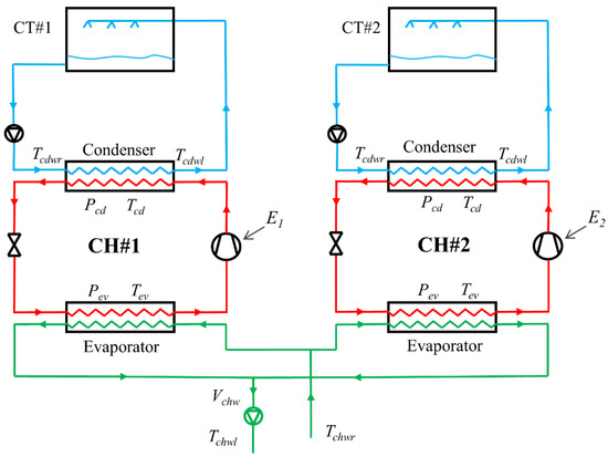
Figure 2.
Schematic of the cooling plant.

Table 1.
Design conditions.
Table 1.
Design conditions.
| Variable | Symbol | Value |
|---|---|---|
| Evaporator cooling load (kW) | Qev,des | 3165 |
| Chiller coefficient of performance (-) | COPdes | 5.76 |
| Electric power input to chiller (kW) | Edes | 549.5 |
| Chilled water leaving temperature (°C) | Tchwl,des | 5.6 |
| Chilled water return temperature (°C) | Tchwr,des | 13.3 |
| Condenser water leaving temperature (°C) | Tcdwl,des | 35.0 |
| Condenser water return temperature (°C) | Tcdwr,des | 29.4 |
| Cooling tower load (kW) | QCT,des | 4540 |
| Volumetric flow rate of chilled water (L/s) | Vchw,des | 72.6 |
| Volumetric flow rate of condenser water (L/s) | Vcdw,des | 131.5 |
BAS records the cooling plant operation every 15 min, and the raw measurements are assigned into three groups based on the three-scenario status. The measured variables from BAS are listed Table 2. Each of the three data groups is further divided into two datasets, i.e., working days and weekend/holidays.
Table 2.
Measurements from the central cooling plant available from BAS for this study.
Table 2.
Measurements from the central cooling plant available from BAS for this study.
| Variable | Symbol |
|---|---|
| Relatively humidity of outdoor air (%) | RHoa |
| Outdoor air temperature (°C) | Toa |
| Chilled water leaving temperature (°C) | Tchwl |
| Chilled water return temperature (°C) | Tchwr |
| Condenser water leaving temperatures (°C) | Tcdwl |
| Condenser water return temperature (°C) | Tcdwr |
| Chilled water volumetric flow rate (L/s) | Vchw |
| Power input to chiller (kW) | E |
| Saturated refrigerant temperature in evaporator (°C) | Tev |
| Refrigerant pressure in evaporator (kPa) | Pev |
| Saturated refrigerant temperature in condenser (°C) | Tcd |
| Refrigerant pressure in condenser (kPa) | Pcd |
The pre-processing verified the raw data quality [30]. Obvious abnormal values (e.g., negative values of Vchw when the chiller operates normally), as well as data under transient condition (e.g., chiller start-up) were removed. Outliers that exceed Chauvenet’s criterion [32] were removed. After the data pre-processing, it was noticed that chiller CH#2 under working days contains the most available measurements (445 measurement data from 11 July 2013 to 26 July 2013). Hence, the chiller CH#2 was selected for the case study.
4.2. Benchmark Model Training and Testing Results
The training data set of normal operation, composed of first 326 measurement data (73% of the whole data set) recorded by BAS every 15 min, from 11 July 2013 to 24 July 2013, are used for the identification of each model parameters with the least squares method (LSM) (Equations (1)–(3)). The remaining 119 measurement data points (27% of the whole data set) are used for the models testing. The benchmarking grey-box models are developed using Python (version 3.9.12) [33] with open-source libraries (e.g., Scikit-learn [34]). The derived benchmark models for the three target variables are summarized in Table 3.
Table 3.
Derived benchmarking grey-box models based on measurements of case study.
Graphical relationships between benchmarking and measured values of the three selected target variable (Figure 3, Figure 4 and Figure 5), and the performance metrics (Equations (4)–(8)) of benchmarking models, calculated over the testing data set, show good prediction performance (Table 4). Results from the augmented and sliding window techniques, not presented in this paper, indicated the three benchmarking models are robust.
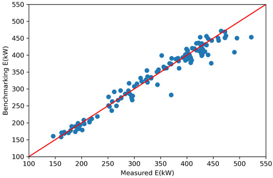
Figure 3.
Benchmarking values of the electric power input E versus measured values over testing data under normal operation conditions.
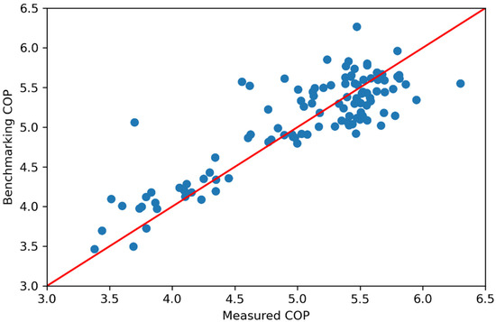
Figure 4.
Benchmarking values of the coefficient of performance COP versus measured values over testing data under normal operation conditions.
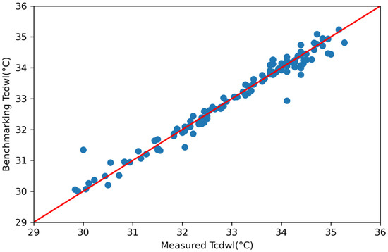
Figure 5.
Benchmarking values of the condenser water leaving temperature Tcdwl versus measured values over testing data under normal operation conditions.
Table 4.
Performance metrics of benchmarking models over testing data set.
The derived models compare well with the actual response of chiller CH#2. For instance, when Tchwl increases, the control system would increase the electric power input to the chiller to maintain the setpoint of Tchwl (Table 3).
The overall uncertainty of measurements was calculated as composed of bias and random errors [35,36] (Table 5). The values that are not available are marked with “NA”. The threshold ε that is used in the fault detection is equal to the overall uncertainty.
Table 5.
Uncertainty of measurements and threshold values derived from the training dataset.
5. Artificial Faults
Detailed records of known equipment faults in existing HVAC system are usually unavailable for research purpose. The building operation team, due to potential disturbances in the operation and occupants’ discomfort, does not easily accept insertion of artificial physical faults in the operation of existing HVAC systems. Several publications present the insertion of numerical artificial faults in the computer simulation models. For instance, a fixed bias of 1 °C was added to the chilled water return temperature sensor in TRANSYS simulator to generate data with a fault [37]. A bias fault of 10 °C and a drifting fault of 0.9 °C/h were injected into simulation results for fault detection using the neural network model [38].
Since there are no faults recorded by the BAS during the chiller operation of this case study, numerical artificial faults are inserted in the measurement data file: (i) the increase in bias error of the chilled water leaving temperature, and (ii) the reduction in refrigerant mass flow rate at the evaporator.
5.1. Artificial Fault of the Measured Chilled Water Leaving Temperature
A bias of 5 °C increase is inserted into the testing dataset for Tchwl over eight-time steps, starting at 13:15:00 on 26 July 2013 and ending at 15:00:00 on 26 July 2013 (Figure 6).
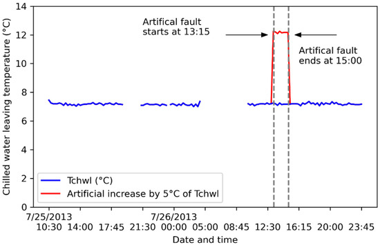
Figure 6.
Artificial increase of 5 °C for Tchwl over eight-time steps, starting at 13:15:00 on 26 July 2013 and ending at 15:00:00 on 26 July 2013.
All the four symptoms (Symp(Tchwl), Symp(E), Symp(COP) and Symp(mev,ref)) are successfully detected (Figure 7, Figure 8, Figure 9 and Figure 10) and they all start from 13:15:00 on 26 July 2013, and end at 15:00:00 on 26 July 2013, which is the same time interval as the artificial Tchwl fault. The FDD model performance metrics are listed in Table 6.
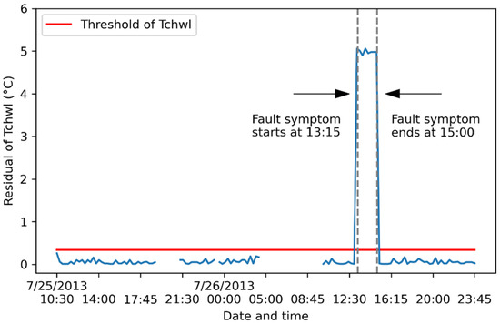
Figure 7.
Impact of artificial fault of Tchwl on the fault symptom of Tchwl. The blue line indicates the absolute values of residual.
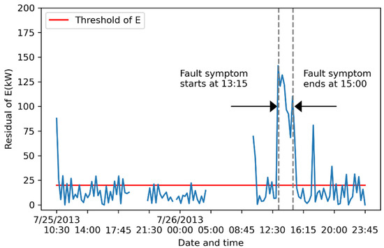
Figure 8.
Impact of artificial fault of Tchwl on the fault symptom of E. The blue line indicates the absolute values of residual.
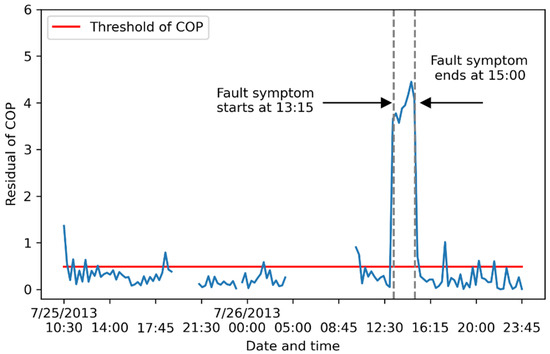
Figure 9.
Impact of artificial fault of Tchwl on the fault symptom of COP. The blue line indicates the absolute values of residual.
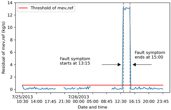
Figure 10.
Impact of artificial fault of Tchwl on the fault symptom of mev,ref. The blue line indicates the absolute values of residual.
Table 6.
Model performance metrics for artificially inserted Tchwl fault, derived from test dataset from 25 July 2013 to 26 July 2013.
HR values for the four symptoms (Symp(Tchwl), Symp(E), Symp(COP), and Symp(mev,ref)) are all 100%. Thus, all the dependent fault symptoms during the period of artificially inserted Tchwl fault, are successfully detected.
Some measurements exceed the threshold ε(E) in fault-free time for E (Figure 8), which results in a relative lower value of AC = 79.0% in terms of Symp(E) (Table 6). These singular points might be due to changes of return chilled water temperature, before the second chiller is turned on. Therefore, such abnormal measurements are not considered as fault symptoms. Same conditions are also noticed in fault detection of Symp(COP) (Figure 9).
As Symp(Tchwl), Symp(E), Symp(COP) and Symp(mev,ref) are detected simultaneously, the variables Tchwl, E, COP and mev,ref appear to be faulty according to fault diagnosis rules. Additional investigation by the operation team is needed.
5.2. Artificial Fault of the Measured Refrigerant Mass Flow Rate
The refrigerant mass flow rate at the evaporator is reduced by 40% due to a fault starting at 13:15:00 on 26 July 2013 and ending at 15:00:00 on 26 July 2013 (Figure 11).
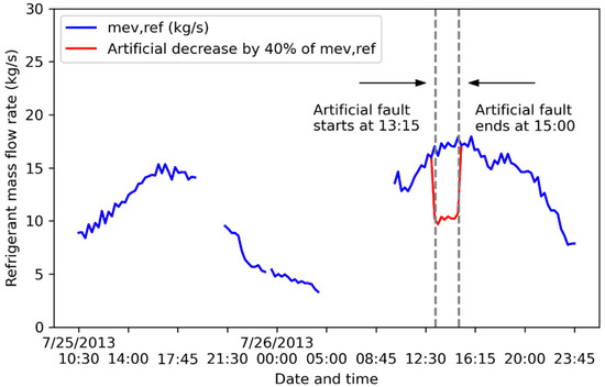
Figure 11.
Artificial decrease by 40% of refrigerant mass flow rate starting at 13:15:00 on 26 July 2013 and ending at 15:00:00 on 26 July 2013.
Symp(E), Symp(COP) and Symp(mev,ref) are successfully detected with high HR values of 100% (Table 7). All symptoms start at 13:15:00 on 26 July 2013 and end at 15:00:00 on 26 July 2013 (Figure 12, Figure 13 and Figure 14), which is the same time interval of artificial mev,ref fault.
Table 7.
Model performance metrics for artificially inserted mev,ref fault, derived from test dataset from 25 July 2013, to 26 July 2013.
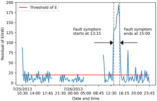
Figure 12.
Impact of artificial fault of mev,ref on the fault symptom of E; the blue line indicates the absolute values of residual of E. The blue line indicates the absolute values of residual.
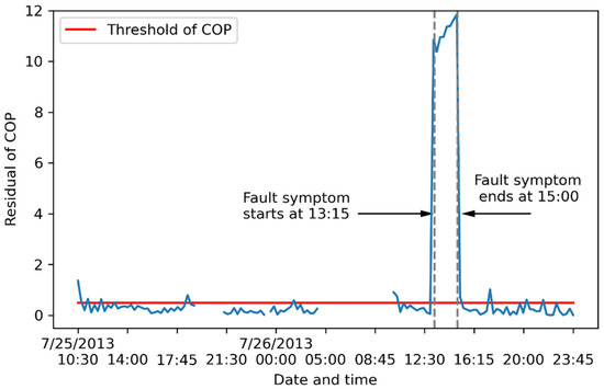
Figure 13.
Impact of artificial fault of mev,ref on the fault symptom of COP; the blue line indicates the absolute values of residual of COP. The blue line indicates the absolute values of residual.
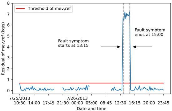
Figure 14.
Impact of artificial fault of mev,ref on the fault symptom of mev,ref; the blue line indicates the absolute values of residual of mev,ref. The blue line indicates the absolute values of residual.
The impact of artificial fault of mev,ref propagates to the two variables of Eb and COPb, which sequentially leads to the detection of Symp(E) and Symp(COP). The impact of artificial mev,ref fault on itself is also identified as Symp(mev,ref) is detected.
In this example, the fault symptoms of E, COP, and mev,ref are detected. According to fault diagnosis rules, the three variables E, COP, and mev,ref are faulty. Additional investigation by the operation team is needed.
6. Conclusions and Future Work
This paper is a contribution to multiple-dependent FDD of chillers using benchmarking grey-box models along with measurement data from BAS of an existing building.
The benchmarking grey-box models for Eb, COPb and Tcdwl.b, are accurate (Table 4). Results of two case studies using artificial faults of Tchwl and mev,ref indicate the proposed model for MDFDD works well by detecting the symptoms of target variables with high hit rate and isolating the source faults successfully. Authors are aware about some limitations of the present work. BAS recordings have a time interval of 15 min, which is not enough for the detection of faults under transient regimes. The proposed method could miss the impact of shorter-time disturbances. Measurement data in this paper only use data over one month (July 2013). Work is currently in progress to explore the chiller operation with measurement data over the whole cooling season.
Although one regressor variable fault (e.g., Tchwl) might have impact on other regressors such as Vchw or/and mev,ref, this paper considers only the significant impact on the target variable (e.g., E). The impact on other regressor variables is neglected. Future work should consider the combined effect of (i) abnormal values of physical variables and (ii) impact on other regressor variables.
Author Contributions
Conceptualization, H.D. and R.Z.; methodology, H.D. and R.Z.; validation, H.D. and R.Z.; investigation, H.D.; resources, R.Z.; data curation, H.D.; writing—original draft preparation, H.D.; writing—review and editing, R.Z. and H.D.; supervision, R.Z.; project administration, R.Z.; funding acquisition, R.Z. All authors have read and agreed to the published version of the manuscript.
Funding
This research was funded by Natural Sciences and Engineering Research Council of Canada grant number [RGOIN.4994-2016], and from Gina Cody School of Engineering and Computer Science grant number [VE0017].
Acknowledgments
The authors acknowledge the financial support from Natural Sciences and Engineering Research Council (NSERC), and Gina Cody School of Engineering and Computer Engineering of Concordia University, Montreal, Canada.
Conflicts of Interest
The authors declare no conflict of interest.
Nomenclature
| BAS | building automation system |
| COP | coefficient of performance |
| CV | coefficient of variance of the RMSE |
| C | specific heat capacity at constant pressure, kJ/(kg·K) |
| E | electric power input to the chiller, kW |
| FDD | fault detection and diagnosis |
| FN | false negative |
| FP | false positive |
| hdis | refrigerant enthalpy at the compressor discharge, kJ/kg |
| hll | refrigerant liquid line enthalpy, kJ/kg |
| hsuc | refrigerant enthalpy at the compressor suction, kJ/kg |
| mev,ref | refrigerant mass flow rate at the evaporator, kg/s |
| MBE | mean bias error |
| MF | multiple faults |
| MDF | multiple dependent faults |
| MDFFD | multiple dependent fault detection and diagnosis |
| MSF | multiple simultaneous faults |
| NMBE | normalized MBE |
| NA | not available |
| PLR | part load ratio |
| Qev | evaporator cooling load, kW |
| r | Pearson coefficient |
| RHoa | outdoor air relative humidity, % |
| RMSE | root of mean square error |
| TN | true negative |
| TP | true positive |
| Tcd | saturated refrigerant temperature at the condenser, °C |
| Tcdwl | condenser water leaving temperature, °C |
| Tcdwr | condenser water return temperature, °C |
| Tchwl | chilled water leaving temperature, °C |
| Tchwr | chilled water return temperature, °C |
| Tdis | compressor discharge temperature, °C |
| Tev | saturated refrigerant temperature at the evaporator, °C |
| Toa | outdoor air temperature, °C |
| Vcdw | condenser water flow rate, m3/s |
| Vchw | chilled water flow rate, m3/s |
| Greek symbols | |
| ε | threshold |
| ρ | water density, kg/m3 |
| Subscript | |
| chw | chilled water |
| cd | condenser |
| cdw | condenser water |
| ev | evaporator |
| m | measured variable |
| b | benchmarking predicted variable |
| ref | refrigerant |
References
- Natural Resources Canada. 2021. Available online: https://oee.nrcan.gc.ca/corporate/statistics/neud/dpa/showTable.cfm?type=HB§or=aaa&juris=ca&rn=2&page=0 (accessed on 6 October 2021).
- Deshmukh, S.; Glicksman, L.; Norford, L. Case study results: Fault detection in air-handling units in buildings. Adv. Build. Energy Res. 2020, 14, 305–321. [Google Scholar] [CrossRef]
- Pe, L. A review on buildings energy consumption information. Energy Build. 2008, 40, 394–398. [Google Scholar] [CrossRef]
- Roth, K.W.; Westphalen, D.; Llana, P.; Feng, M. The energy impact of faults in US commercial buildings. In Proceedings of the International Refrigeration and Air Conditioning Conference, West Lafayette, IN, USA, 12–15 July 2004. [Google Scholar]
- Rogers, A.P.; Guo, F.; Rasmussen, B.P. A review of fault detection and diagnosis methods for residential air conditioning systems. Build. Environ. 2019, 161, 106236. [Google Scholar] [CrossRef]
- Li, L.; Luo, H.; Ding, S.X.; Yang, Y.; Peng, K. Performance-based fault detection and fault-tolerant control for automatic control systems. Automatica 2019, 99, 308–316. [Google Scholar] [CrossRef]
- Qu, J.; Zhang, H.; Zhang, G.; Chen, H. Incipient fault detection of chiller based on improved CVA. E3S Web Conf. 2021, 257, 01062. [Google Scholar] [CrossRef]
- Gunay, H.B.; Shen, W.; Yang, C. Text-mining building maintenance work orders for component fault frequency. Build. Res. Inf. 2019, 47, 518–533. [Google Scholar] [CrossRef]
- Yu, Y.; Woradechjumroen, D.; Yu, D. A review of fault detection and diagnosis methodologies on air-handling units. Energy Build 2014, 82, 550–562. [Google Scholar] [CrossRef]
- Suttell, R. Preventive HVAC maintenance is a good investment. Buildings 2006, 100, 50–52. [Google Scholar]
- Rich, S.H.; Venkatasubramanian, V. Causality-based failure-driven learning in diagnostic expert systems. AIChE J. 1989, 35, 943–950. [Google Scholar] [CrossRef]
- Mckellar, M.G.; Tree, D.R. Steady State Characteristics of Failures of a Household Refrigerator. In Proceedings of the International Refrigeration and Air Conditioning Conference, Purdue, Indiana, 18–21 July 1988. [Google Scholar]
- Kim, W.; Katipamula, S. A review of fault detection and diagnostics methods for building systems. Sci Technol Built Environ. 2018, 24, 3–21. [Google Scholar] [CrossRef]
- Fernandez, N.; Brambley, M.R.; Katipamula, S.; Cho, H.; Goddard, J.; Dinh, L. Self-Correcting HVAC Controls Project Final Report; Pacific Northwest National Lab.: Richland, WA, USA, 2010.
- Brambley, M.R.; Cort, K.A.; Goddard, J.K.; Fernandez, N.; Cho, H.; Wang, W. Final Project Report: Self-Correcting Controls for VAV System Faults Filter/Fan/Coil and VAV Box Sections; Pacific Northwest National Lab.: Richland, WA, USA, 2011.
- Weimer, J.; Ahmadi, S.A.; Araujo, J.; Mele, F.M.; Papale, D.; Shames, I.; Sandberg, H.; Johansson, K.H. Active actuator fault detection and diagnostics in HVAC systems. In Proceedings of the 4th ACM Workshop on Embedded Sensing Systems for Energy-Efficiency in Buildings, Toronto, ON, Canada, 6 November 2012; pp. 107–114. [Google Scholar]
- Bruton, K.; Raftery, P.; O’Donovan, P.; Aughney, N.; Keane, M.M.; O’Sullivan, D.T.J. Development and alpha testing of a cloud based automated fault detection and diagnosis tool for Air Handling Units. Autom. Constr. 2014, 39, 70–83. [Google Scholar] [CrossRef]
- Ngaopitakkul, A.; Apisit, C.; Bunjongjit, S.; Pothisarn, C. Identifying types of simultaneous fault in transmission line using discrete wavelet transform and fuzzy logic algorithm. Int. J. Innov. Comput. Inf. Control 2013, 9, 2701–2712. [Google Scholar]
- Lee, G.; Lee, B.; Yoon, E.S.; Han, C. Multiple-fault diagnosis under uncertain conditions by the quantification of qualitative relations. Ind Eng Chem. Res. 1999, 38, 988–998. [Google Scholar] [CrossRef]
- Du, Z.; Jin, X. Detection and diagnosis for multiple faults in VAV systems. Energy Build. 2007, 39, 923–934. [Google Scholar] [CrossRef]
- Wang, H.; Chen, Y. A robust fault detection and diagnosis strategy for multiple faults of VAV air handling units. Energy Build 2016, 127, 442–451. [Google Scholar] [CrossRef]
- Breuker, M.S.; Braun, J.E. Common Faults and Their Impacts for Rooftop Air Conditioners. HVAC&R Res. 1998, 4, 303–318. [Google Scholar] [CrossRef]
- Li, H.; Braun, J.E. A methodology for diagnosing multiple simultaneous faults in vapor-compression air conditioners. HVAC&R Res. 2007, 13, 369–395. [Google Scholar] [CrossRef]
- Li, H.; Braun, J.E. Decoupling features and virtual sensors for diagnosis of faults in vapor compression air conditioners. Int. J. Refrig. 2007, 30, 546–564. [Google Scholar] [CrossRef]
- Li, H.; Braun, J.E. Decoupling features for diagnosis of reversing and check valve faults in heat pumps. Int. J. Refrig. 2009, 32, 316–326. [Google Scholar] [CrossRef]
- Kim, W.; Braun, J.E. Development, implementation, and evaluation of a fault detection and diagnostics system based on integrated virtual sensors and fault impact models. Energy Build. 2020, 228, 110368. [Google Scholar] [CrossRef]
- Katipamula, S.; Brambley, M.R. Methods for fault detection, diagnostics, and prognostics for building systems—A review, part I. HVAC&R Res. 2005, 11, 3–25. [Google Scholar] [CrossRef]
- Han, H.; Gu, B.; Wang, T.; Li, Z.R. Important sensors for chiller fault detection and diagnosis (FDD) from the perspective of feature selection and machine learning. Int. J. Refrig. 2011, 34, 586–599. [Google Scholar] [CrossRef]
- Lee, D.; Lai, C.W.; Liao, K.K.; Chang, J.W. Artificial intelligence assisted false alarm detection and diagnosis system development for reducing maintenance cost of chillers at the data centre. J. Build. Eng. 2021, 36, 102110. [Google Scholar] [CrossRef]
- Han, J.; Pei, J.; Kamber, M. Data Mining: Concepts and Techniques. Elsevier: Amsterdam, The Netherlands, 2011. [Google Scholar]
- Monfet, D.; Zmeureanu, R. Ongoing commissioning of water-cooled electric chillers using benchmarking models. Appl. Energy 2012, 92, 99–108. [Google Scholar] [CrossRef]
- Dou, H.; Zmeureanu, R. Evidence-based assessment of energy performance of two large centrifugal chillers over nine cooling seasons. Sci. Technol. Built. Environ. 2021, 27, 1243–1255. [Google Scholar] [CrossRef]
- Python Release Python 3.9.12|Python.org n.d. Available online: https://www.python.org/downloads/release/python-3912/ (accessed on 1 September 2022).
- Scikit-Learn: Machine Learning in Python—Scikit-Learn 1.1.2 Documentation. Available online: https://scikit-learn.org/stable/ (accessed on 1 September 2022).
- Guideline 2-2010; Engineering Analysis of Experimental Data. American Society of Heating. Refrigerating and Air-Conditioning Engineers, Inc.: Atlanta, GA, USA, 2010.
- Reddy, T.A. Applied Data Analysis and Modeling for Energy Engineers and Scientists; Springer: New York, NY, USA, 2011. [Google Scholar]
- Du, Z.; Fan, B.; Jin, X.; Chi, J. Fault detection and diagnosis for buildings and HVAC systems using combined neural networks and subtractive clustering analysis. Build. Environ. 2014, 73, 1–11. [Google Scholar] [CrossRef]
- Elnour, M.; Meskin, N.; Al-naemi, M. Sensor data validation and fault diagnosis using Auto-Associative Neural Network for HVAC systems. J. Build. Eng. 2020, 27, 100935. [Google Scholar] [CrossRef]
Disclaimer/Publisher’s Note: The statements, opinions and data contained in all publications are solely those of the individual author(s) and contributor(s) and not of MDPI and/or the editor(s). MDPI and/or the editor(s) disclaim responsibility for any injury to people or property resulting from any ideas, methods, instructions or products referred to in the content. |
© 2022 by the authors. Licensee MDPI, Basel, Switzerland. This article is an open access article distributed under the terms and conditions of the Creative Commons Attribution (CC BY) license (https://creativecommons.org/licenses/by/4.0/).