A Novel Workflow for Early Time Transient Pressure Data Interpretation in Tight Oil Reservoirs with Physical Constraints

Abstract

In this work, a novel workflow has been proposed, validated and applied to interpret the early time transient pressure data in tight oil reservoirs with physical constraints. More specifically, the theoretical model was developed to obtain the transient pressure response for a vertical well in tight oil reservoirs with consideration of pseudo threshold pressure gradient (TPG). Then, a physical constraint between the skin factor and formation permeability has been proposed based on the physical meaning of percolation theory. This physical constraint can be applied to determine the lower limit of the skin factor which can reduce the uncertainty during the interpretation process. It is found that the influence range of the skin factor and permeability may partially overlap during the interpretation process without consideration of physical constraints. Additionally, it is found that the equivalent wellbore radius is more reasonable by considering the skin factor constraints. Furthermore, the short-time asymptotic method was applied to separate the small pressure signal at the early time period and a novel type curve was proposed to better analyze the early time pressure response. Subsequently, sensitivity analyses were conducted to investigate the influence of different parameters on the new type curves. It is found that the new type curves are more dispersed and sensitive to the parameters at the early time period which can be beneficial for the early time transient pressure analysis in a tight formation. The proposed method has been validated and then extended to a field application, demonstrating that the transient pressure for a vertical well in a tight formation can be analyzed in a reasonable and accurate manner with only early time transient pressure data.

1. Introduction

Due to the declining reserves of conventional reservoirs and the growing global energy consumption, unconventional resources have received increasing reliance [1]. As tight oil reservoirs account for a significant portion of unconventional hydrocarbon resources, the efficient development of tight oil reservoirs has become a primary focus [2,3]. Pressure transient analysis is considered to be a valuable method to provide information about reservoirs by interpreting the pressure data [4,5,6]. For pressure transient analysis, the reservoir properties can be estimated or determined by identifying different flow regimes on the pressure derivative curve [7,8,9,10]. Since the permeability of a tight oil reservoir is extremely low, it usually takes quite a long time to achieve the infinite acting radial flow (IARF) regime and the early time transient pressure data can be difficult to interpret which makes the well testing method less attractive [11]. Therefore, the traditional pressure transient analysis method is not applicable to tight oil reservoirs and it is of fundamental and practical importance to find an appropriate method to analyze the early time transient pressure data in the tight formation in a consistent and accurate manner.

The low-velocity non-Darcy flow phenomenon can be described by the curves shown in Figure 1 where the red curve represents the traditional Darcy flow. However, at the lower pressure gradient region, fluid cannot flow through the porous media unless the pressure gradient exceeds the threshold pressure gradient (TPG). At the region where the pressure gradient larger than TPG, a linear relationship between the flow velocity and pressure gradient can be found. The existence of TPG has been observed from laboratory works [12,13] which can be explained by the effect of tight pore structures, non-Newtonian fluid, and boundary layer [14,15]. Many factors, including pore-throat size, capillary pressure, fluid saturation, and permeability can affect the value of threshold pressure gradient in a tight formation, and the reasonable range of threshold pressure gradient in a tight formation has been reported to be 0.006–0.04 MPa/m [16,17,18]. The TPG can not only result in nonlinear and nonhomogeneous diffusivity equations which are difficult to solve but also can affect the production performance of the tight formations [19]. Numerous attempts have been made to investigate the transient pressure behavior by considering the TPG through both numerical and analytical methods [7,20,21]. However, it is found that the TPG mainly affects the flow regime at late time periods where little information about the TPG can be found from analyzing the early time transient pressure data [7,21]. In order to better understand the reservoir properties with consideration of TPG from the transient pressure analysis method, it is urgent to seek a trustworthy method for such a purpose.

As the lower permeability and poor flow capacity in a tight formation, it is difficult to reach the IARF regime for the well testing method where long time pressure testing operation will seriously affect the well production [11]. As such, the early time transient pressure data without enough information about the IARF regime are usually obtained during the well testing method for a tight formation [7]. For the early time transient pressure response, usually three parameters dominate the early time pressure response including the wellbore storage coefficient, skin factor, and reservoir permeability. For the latter two parameters, it is usually hard to separate their respective influence on the transient pressure curves, and there is no physical constraint for the lower limit of skin factor (usually between −6–100) [22] which can bring high ambiguity for the well testing interpretation results. Efforts have been made to analyze the early time trainset rate/pressure data by using various new type curves under various conditions for various reservoirs [23,24,25]. However, the TPG is usually neglected for such reservoirs which may greatly affect the transient pressure behavior for a tight formation.

In this work, a numerical model has been proposed and validated to investigate the effect of TPG, wellbore storage, and skin factor on the early time transient pressure response for a tight formation. The physical constraint for the skin factor has been proposed which can reduce the uncertainty of the interpretation results. Furthermore, a novel type curve has been developed which is capable to extract the small pressure signal at the early time period. Based on the new type curves, sensitivity analyses have been done to examine the effect of TPG, wellbore storage, and skin factor for both Darcy flow model and low-velocity non-Darcy flow model.

2. Methodology

In this work, a vertical well is located in a cylindrical tight oil reservoir with infinite boundary (see Figure 2), and the main assumptions are listed as follows,

(1)

The infinite reservoir is homogeneous with constant thickness;

(2)

Slightly compressible single phase fluid is assumed in the formation;

(3)

Fluid flow in the formation obeys the low-velocity non-Darcy flow characterized by TPG;

(4)

The well production rate is constant during the production periods; and

(5)

Wellbore storage and skin factor are considered, and gravity effect is ignored in this work.

2.1. Analytical Solution

The vertical well fully penetrates the formation, and the gravity effect is ignored in this work. Thus, only the radial flow towards the vertical wellbore is considered which can accurately describe the fluid flow behavior in such a reservoir, while the vertical flow can be neglected in this work. The governing equation for the isotropic reservoir with consideration of pseudo TPG can be written as follows, and the detailed derivation can be found in Appendix A,

$$\{\begin{array}{c}\frac{{\partial }^{2}p}{\partial r^2}+\frac{1}{r}\frac{\partial p}{\partial r}-\frac{1}{r}\lambda =\frac{\varphi \mu C_t}{k}\frac{\partial p}{\partial t}\\ {p(r,t)|}_{t=0}=p_i\\ \underset{r\to \infty }{\lim }p(r,t)=p_i\\ qB={\left[\frac{2\pi rhk}{\mu }(\frac{\partial p}{\partial r}-\lambda )\right]}_{r=r_{we}}-C\frac{d{p}_w}{dt}\\ p_w=p(r_{we},t)\end{array}$$

(1)

where p is formation pressure, r is the distance away from the wellbore, ϕ is formation porosity, μ is fluid viscosity, C_t is total formation compressibility, k is the formation permeability, t is real time, λ is the pseudo TGP, B is the oil formation volume factor, p_i is the initial formation pressure, p_w is the well bottom-hole pressure (BHP), C is the wellbore storage coefficient, S is the sin factor, and r_we is the equivalent wellbore radius (i.e., r_{we =} r_we^−S).

The following dimensionless variables are defined for further analysis,

$$p_D=\frac{2\pi kh(p_i-p)}{qB\mu },t_D=\frac{kt}{\varphi \mu C_t{r}_w^2},r_D=\frac{r}{r_w{e}^{-S}},C_D=\frac{C}{2\pi h\varphi C_t{r}_w^2},{\lambda }_{\mathrm{D}}=\frac{2\pi kh{r}_w\lambda }{qB\mu }$$

(2)

Then, the dimensionless governing equations together with the boundary and initial conditions can be obtained as follows,

$$\{\begin{array}{c}\frac{{\partial }^2{p}_D}{\partial r_D^2}+\frac{1}{r_D}\frac{\partial p_D}{\partial r_D}+\frac{{\lambda }_{\mathrm{D}}{e}^{-S}}{r_D}=\frac{1}{C_D{e}^{2S}}\frac{\partial p_D}{\partial (t_D/C_D)}\\ p_D(r_D,t_D/C_D){|}_{t_D/C_D=0}=0\\ \underset{r_D\to \infty }{\lim }{p}_D(r_D,t_D/C_D)=0\\ \frac{\partial p_{wD}}{\partial (t_D/C_D)}-{\frac{\partial p_D}{\partial r_D}|}_{r_D=1}=1+{\lambda }_{\mathrm{D}}{e}^{-S}\\ p_{wD}=p_D(1,t_D/C_D)\end{array}$$

(3)

The Laplace transform is applied with respect to t_D/C_D, which is

$${\overline{p}}_D={\displaystyle {\int }_0^{\infty }{p}_D{e}^{-u{t}_D/C_D}d(t_D/C_D})$$

(4)

Therefore, the corresponding Laplace transform of the aforementioned governing equations can be further acquired,

$$\{\begin{array}{c}\frac{{\partial }^2{\overline{p}}_{\mathrm{D}}}{\partial r_{\mathrm{D}}^2}+\frac{1}{r_{\mathrm{D}}}\frac{\partial {\overline{p}}_{\mathrm{D}}}{\partial r_{\mathrm{D}}}+\frac{{\lambda }_{\mathrm{D}}{e}^{-s}}{u{r}_D}=\frac{u}{C_D{e}^{2S}}{\overline{p}}_{\mathrm{D}}\\ {\overline{p_D}(r_D,u)|}_{r_D\to \infty }=0\\ u{\overline{p}}_{wD}-{\frac{\partial {\overline{p}}_{\mathrm{D}}}{\partial r_D}|}_{r_D=1}=\frac{1+{\lambda }_{\mathrm{D}}{e}^{-S}}{u}\\ {\overline{p}}_{wD}={\overline{p}}_{\mathrm{D}}(1,u)\end{array}$$

(5)

As the governing equations are nonhomogeneous due to the existence of TPG, and the general form of the solution for the governing equations can be written in the following form on the basis of the Bessel functions,

$${\overline{p}}_{\mathrm{D}}(r_D)=A\cdot I_0(\beta r_D)+B{K}_0(\beta r_D)+\frac{M}{\beta }{K}_0\left(\beta r_{\mathrm{D}}\right){\displaystyle {\int }_{\beta }^{\beta r_{\mathrm{D}}}{I}_0\left(\xi \right)}d\xi +\frac{M}{\beta }{I}_0\left(\beta r_{\mathrm{D}}\right){\displaystyle {\int }_{\beta r_{\mathrm{D}}}^{\infty }{K}_0\left(\xi \right)}d\xi$$

(6)

where M = λ_De^−S, β = (u/C_De^2S)^0.5, I₀(x), and K₀(x) are the zero-order modified Bessel function of the first and second kind, respectively.

By applying the boundary conditions, the constant A and B can be inversely obtained. Then, the analytical pressure solution in the Laplace domain can be written as follows,

$$\begin{array}{l}{\overline{p}}_{wD}=\frac{K_0(\beta )}{u{K}_0(\beta )+\beta K_1(\beta )}\left[\frac{1+{\lambda }_{\mathrm{D}}{e}^{-S}}{u}-u\frac{M}{\beta }{I}_0\left(\beta \right){\displaystyle {\int }_{\beta }^{\infty }{K}_0\left(\xi \right)}d\xi +M{I}_1\left(\beta \right){\displaystyle {\int }_{\beta }^{\infty }{K}_0\left(\xi \right)}d\xi \right]\\ \\ +\frac{M}{\beta }{I}_0\left(\beta \right){\displaystyle {\int }_{\beta }^{\infty }{K}_0\left(\xi \right)}d\xi \end{array}$$

(7)

where I₁(x), and K₁(x) are the first-order modified Bessel function of the first and second kind, respectively. After obtaining the pressure solution in the Laplace domain, the well bottom hole pressure solution in the real-time domain p_wD can be inversely calculated by the Stehfest inverse algorithm [26]. In this work, to obtain more precise pressure solutions for the early time periods, the Stehfest number is chosen to be 12.

2.2. Skin Factor Constraint

Skin factor is used to characterize the near wellbore conditions and the connectivity between the well and the formation. The positive and negative skin factors represent the damaged and stimulated near wellbore conditions. Usually, the range of skin factor can be treated in the range of −6~+100 in the practical case [17]. However, no theoretical proof has been made to define the lower limit of this factor, and the very low skin factor can produce unrealistic or unphysical phenomenon even though the transient pressure data has been well matched. In this work, the lower limit of the skin factor can be theoretically obtained which can apparently reduce the ambiguity during the pressure data matching process, especially with a relatively short testing duration.

The definition of the skin factor is [22],

$$\Delta p_{skin}=\left[p{\left(r_w,t\right)}_{ideal}-p{\left(r_w,t\right)}_{actual}\right]=S\frac{q\mu }{2\pi kh}$$

(8)

where p(r_w,t)_ideal is the BHP for the ideal case, and p(r_w,t)_actual is the BHP for the actual case.

For the ideal case without skin factor, the analytical solution can be written as follows,

$$p{\left(r_w,t\right)}_{ideal}=p_i-\frac{q\mu }{4\pi kh}\left[-Ei\left(-\frac{r_w^2}{4\eta t}\right)\right]$$

(9)

where η is the pressure diffusivity coefficient (i.e., η = k/(ϕμC_t)). Substitute Equation (9) into Equation (8), we can obtain,

$$p_i-p{\left(r_w,t\right)}_{actual}=\frac{q\mu }{4\pi kh}\left[-Ei\left(-\frac{r_w^2}{4\eta t}\right)\right]+S\frac{q\mu }{2\pi kh}$$

(10)

For the practical case, the BHP cannot be higher than the initial pressure after production, and the following physical constraint can be obtained,

$$S>\frac{1}{2}Ei\left(-\frac{r_w^2}{4\eta t}\right)$$

(11)

The exponential integral function Ei(−x) is inconvenient for practical use, when 0 < x ≤ 0.01, Ei(−x) can be approximated as the following form with high accuracy (see Figure 3).

$$\begin{array}{cc}Ei\left(-x\right)\approx -\ln \frac{e^{-0.5772}}{x},& 0<x\end{array}\le 0.01$$

(12)

Additionally, as the function Ei(−x) is negative, and the larger the absolute value of x the smaller the value of Ei(−x). Thus, the following constraint of skin factor can be obtained,

$$S\{\begin{array}{cc}>\frac{1}{2}Ei\left(-0.01\right)& \frac{r_w^2}{4\eta t}\ge 0.01\\ >-\frac{1}{2}\ln \left(\frac{2.25\eta t}{r_w^2}\right)& \frac{r_w^2}{4\eta t}<0.01\end{array}$$

(13)

In the field well-testing application, the minimum test time is chosen to be 10 s which is smaller enough for the transient pressure test data obtained. As the time becomes larger, the smaller value of $r_w^2$/(4ηt) can result in a smaller value of the lower limit of skin factor. To maintain the physical constraint for the whole testing period, the lower limit for the skin factor can be further obtained as follows,

$$S\{\begin{array}{cc}>-2\begin{array}{cc}\begin{array}{cc}& \end{array}& \end{array}& \frac{r_w^2}{4\eta }\ge 0.1\\ >-\frac{1}{2}\ln \left(\frac{22.5\eta }{r_w^2}\right)& \frac{r_w^2}{4\eta }<0.1\end{array}$$

(14)

Now, the constraints for the skin factor have been theoretically obtained which can be convenient for the practical application during the well-testing interpretation process.

2.3. Applicability Analysis of G-B Type Curves

Gringarten et al. [27] improved the Agarwal-Ramey type curves [28] and obtained the Gringarten type curves. Then, Bourdet et al. [29] creatively proposed the Bourdet pressure derivative (i.e., p’_wD = dp_wD/dln(t_D/C_D)) curves, and later the two type curves were combined into Gringarten-Bourdet type curves. The G-B type curves can describe the transient pressure behavior for a vertical well with a constant wellbore storage coefficient and skin factor in a reservoir with an infinite outer boundary. The dimensionless pressure and the pressure derivative functions are both plotted as a function of dimensionless time t_D/C_D in a single chart (see Figure 4). This chart is easy to distinguish reservoir types and flow stages, making it easier to obtain a unique fitting curve.

For the transient pressure analysis, the main flow regime of interest is the infinite acting radial flow (IARF) which can be easily identified from the log-log plot (i.e., horizontal line with Bourdet derivative equals 0.5). Additionally, combined the early time wellbore storage regime (i.e., unit slope line) with the IARF regime, the fitting or match of the pressure response would be more immediate and unique. However, there are several limitations during the well test interpretation process for tight formations. For example, in a tight formation with permeability equals 0.5 mD, reservoir thickness of 10 m, viscosity of 0.5 mPa·s, and wellbore storage coefficient of 0.5 m³/MPa, the dimension time t_D/C_D equals 160 when the testing time equals 15 days. As shown in the following G-B type curves, the IARF regime cannot be reached even though the testing time has lasted for 15 days. If the IARF regime shall be shown on the log-log plot, the test time would be up to 100 days, which would obviously and seriously impact the well production and make the well testing method unattractive for the tight formations. Therefore, it is of fundamental and practical significance to find a method to interpret the early time transient pressure response without a possible IARF regime.

2.4. Short-Time Asymptotic Solution

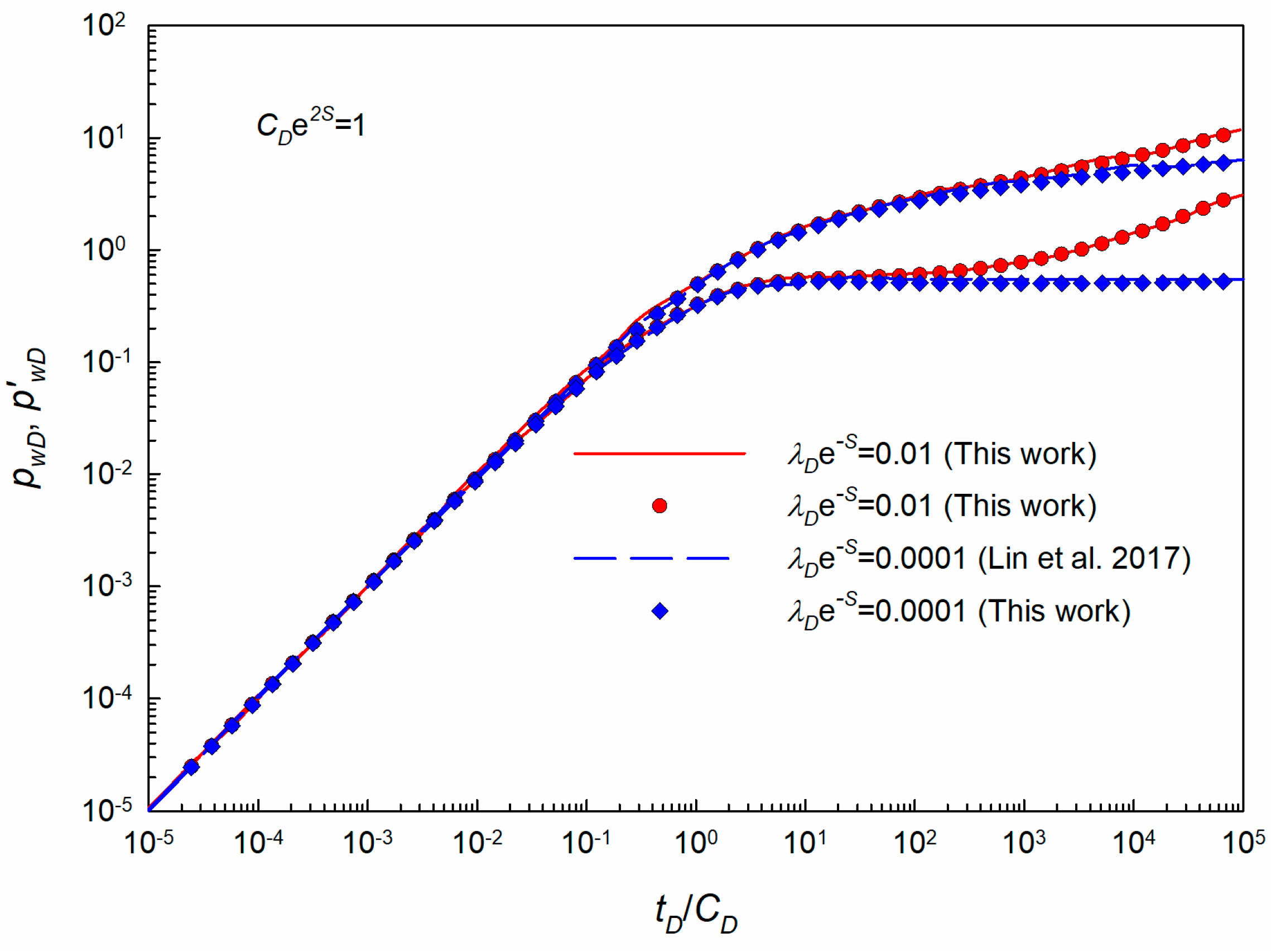
For the early time transient pressure data, it is very difficult for us to identify the wellbore storage and skin factor as the pressure and its derivative curves usually overlap in a unit-slope line for the traditional G-B type curves. Recall that the pressure derivative proposed by Bourdet et al. [29] the essence of this term is actually a mathematical transformation that can separate the small pressure variance and then amplify this small signal through the product of time. The larger the time, the greater the amplification factor becomes. However, this transformation is not valid for the early time period as the pressure derivative approximately equals t_D/C_D resulting in a unit-slope line. Therefore, for the pressure response data without radial flow regimes, strong no-uniqueness can be found during the transient pressure interpretation process.

Based on the idea of Bourdet’s pressure derivative, we want to extract the influence factor at the early times which is more sensitive on the C_D, S, and λ_D by mathematic transformation. The short-time asymptotic method can be applied to obtain this objective. The early time pressure solution is expanded and only the high-order series of the solution is separated which represents the small signal during the early time. In this way, more accurate type curves can be obtained which may be more sensitive on C_D, S, and λ_D during the early times and can obviously reduce the non-uniqueness of the interpretation results.

When the time is relatively smaller in the real-time domain, the Laplace variable u and β can be very large in the Laplace domain. Thus, the K₀(x) and K₁(x) can be asymptotically expanded as follows when β → 0 [30],

$$\begin{array}{cc}{K}_0\left(\beta \right)=\sqrt{\frac{\pi }{2\beta }}{e}^{-\beta }\left[1-\frac{1}{8\beta }+O\left({\beta }^{-1}\right)\right],& K_1\left(\beta \right)=\sqrt{\frac{\pi }{2\beta }}{e}^{-\beta }\left[1+\frac{3}{8\beta }+O\left({\beta }^{-1}\right)\right]\end{array}$$

(15)

Substitute Equation (14) into the solution in Equation (7), we have,

$${\overline{p}}_{wD}=\left(1+{\lambda }_{\mathrm{D}}{e}^{-S}\right)\left[u^{-2}-\frac{1}{\sqrt{C_D{e}^{2S}}}{u}^{-5/2}+O\left(u^{-5/2}\right)\right]$$

(16)

Neglecting the high-order term with small value, then transforming the solution to the real-time domain with respect to t_D/C_D yields,

$$p_{wD}=\left(1+{\lambda }_{\mathrm{D}}{e}^{-S}\right)\left[\frac{t_D}{C_D}-\frac{4}{3\sqrt{\pi C_D{e}^{2S}}}{\left(\frac{t_D}{C_D}\right)}^{3/2}\right]$$

(17)

Based on the idea of parameters proposed in the literature [30], a novel parameter was defined to amplify the small variable for the early time solution in Equation (17) in this work,

$$\omega =\left|\frac{3}{2}\frac{p_{wD}}{t_D/C_D}-\frac{1}{2}\frac{d{p}_{wD}}{d\left(t_D/C_D\right)}-1\right|=\left|{\lambda }_{\mathrm{D}}{e}^{-S}-\frac{\left(1+{\lambda }_{\mathrm{D}}{e}^{-S}\right)}{\sqrt{\pi C_D{e}^{2S}}}{\left(\frac{t_D}{C_D}\right)}^{1/2}\right|$$

(18)

It can be found from the above equation that only the contribution of C_D, S, and λ_D are considered, and these constructed curves are more sensitive to C_D, S, and λ_D other than a unit slope line with little information in the G-B type curves for the early times. Additionally, this curve has a horizontal asymptote (i.e., λ_De^−S) as the time t_D/C_D approaches zero when the TPG is considered. If TPG is not considered, this curve approaches the line (t_D/C_D)^0.5/(πC_De^2S)^0.5 when the time is small.

3. Model Validation

To verify the solutions obtained in this work, the transient pressure behavior was compared with those from previous work [31]. The low-velocity non-Darcy flow model was considered for the tight formation with the following main parameter, C_De^2S = 1, λ_De^-S = 0.0001, 0.01. As shown in Figure 3, there exists a good agreement between the results from this work and those from the literature confirming the accuracy of the solutions in this work to model the transient pressure behavior in a tight formation with consideration of the pseudo TPG. Additionally, it can be found from Figure 5, the existence of TPG can result in an increase of pressure and its derivative curves at the late time period. Additionally, the traditional IARF regime with a horizontal line at late times cannot be observed which can cause more uncertainty during the well-testing interpretation process as the most important flow regime characteristic (i.e., horizontal line with Bourdet derivative equals 0.5) has been changed due to the existence of TPG.

4. Results and Discussion

In this section, the rationality of the skin factor constraints has been clarified, and the novel type curves suitable for the early time transient pressure analysis have been generated. The sensitivity analysis has been conducted to investigate the effects of some main parameters on the new type curves.

4.1. Reasonability Analysis for the Physical Constraint of Skin Factor

During the well testing interpretation for the tight oil reservoirs, the constraint conditions of skin factor are usually not considered, which would lead to doubts about the interpretation results. Specifically, the skin factor reflects the pollution or improvement in the vicinity of the wellbore, and the permeability near the wellbore region represents the seepage capacity of the formation. The conceptual scope of these two should be different.

Table 1. Interpretation results for the transient pressure with and without skin factor constraints.

Well Name	Without Constraints		With Constraints
	Skin Factor	Permeability/mD	Skin Factor	Permeability/mD
Well1	−2.88	4.22	−0.45	10.67
Well2	−3.79	5.23	−0.50	25.06
Well3	−3.82	1.20	−0.11	8.59
Well4	−4.89	1.90	−0.50	35.60
Well5	−3.74	1.78	−0.60	7.08
Well6	−3.12	6.93	−0.50	20.00
Well7	−3.02	4.48	−0.50	29.40
Well8	−2.82	6.45	−0.50	23.10
Well9	−3.64	3.59	−0.50	10.28
Well10	−3.22	3.06	−0.01	8.16
Well11	−3.32	15.73	−0.75	62.75
Well12	−3.65	10.11	−0.25	72.00
Well13	−3.60	8.99	−0.75	24.75
Well14	−3.00	1.21	−0.36	5.62
Well15	−4.50	0.95	−0.50	2.57
Well16	−4.66	1.05	−0.50	6.93
Well17	−3.75	8.51	−0.50	9.95
Well18	−2.60	0.40	−0.50	0.37
Well19	−3.61	0.26	0.28	0.84
Well20	−2.71	1.55	0.12	1.67
Well21	−4.18	2.35	−0.40	11.70
Well22	−2.75	0.22	−0.50	0.63
Well23	−3.68	0.08	−0.50	0.65

shows the interpretation results of a typical tight oil reservoir in the eastern part of China (the case where the skin factor is obviously abnormal and less than −5 has been removed). The current interpretation results have proved that the (inner zone) permeability can be greatly affected by the value of the skin factor. It can be found from the following table that the skin factor is between −4.89 and −2.60 when the skin factor constraint conditions are not considered, resulting in the corresponding equivalent well diameter between 0.8~8.0 m, and the average permeability is 3.92 mD. When considering the skin factor constraints, the skin factor is between −0.75~0.28, and the corresponding equivalent well diameter is between 0.05~0.13 m, and the average permeability is 16.45 mD.

From a numerical point of view, the equivalent well diameter is more reasonable after considering the constraint conditions of the skin factor. Moreover, as the value of the skin factor has been confined to guarantee the correctness of the pressure solution, the influence of the skin factor can be greatly excluded for the early time transient pressure response which brings little interference to the interpretation of the permeability for the near wellbore region. As shown in Figure 6, the permeability obtained after considering the constraints of the skin factor is about 4 times that of the original result without constraints, which can reflect a more realistic seepage capacity of the formation near the wellbore which may be artificially fractured.

4.2. Sensitivity Analysis Based on New Type Curves

4.2.1. New Type Curves for Darcy Flow Model

The low-velocity non-Darcy flow is not considered and the new type curves for the Darcy flow model are generated (i.e., λ_D = 0). The main parameters affecting the type curves are the combination of C_D and S which are the same as the G-B type curves. However, a new curve reflecting the relationship between the newly defined parameter ω and the dimensionless time t_D/C_D is added to the traditional G-B type curves. Figure 7 shows the influence of parameter C_De^2S on the new type curves. It can be found at the early time wellbore storage (WBS) regime, all the pressure and its derivative curves are coinciding lines with unit-slope, little information can be obtained from the transient pressure response during this period only by analyzing the pressure and pressure derivative curves. The following flow regime is the transient flow regime which can be affected by the skin factor and the permeability. The larger the value of C_De^2S, the higher the position of the pressure and its derivative curves. However, the differences in the pressure and its derivative curves during the transition flow regime between different cases are not large enough which can bring high uncertainty for the well testing analysis and interpretation. The last flow regime is the IARF regime, all the pressure derivative curves overlap with a horizontal line for different cases. However, such flow regime is difficult to appear for the well testing in a tight formation where the low permeability can greatly delay its arrival.

The green lines in Figure 7 represent the relationship between the newly defined parameter ω and the dimensionless time t_D/C_D. It can be found that these ω curves can be highly dispersed at the early time period which can be beneficial to the analysis and interpretation of the early time pressure response. The ω curves are sensitive for the parameter C_De^2S at the early time period, and such new curves can be used for the early time transient pressure analysis. Additionally, it can be found that all the ω curves coincide into a horizontal line with its value equals unity. Even though it can be treated as a characteristic line similar to the horizontal derivative line in IARF regime, it is not very useful for the analysis of the early time pressure response where such a horizontal line may be not present within a limited testing time. Moreover, it can be found that the ω curve shows a straight line and its slope is affected by the value of C_De^2S which has been discussed early after the definition of this parameter.

4.2.2. Effect of C_De^2S on New Type Curves for Non-Darcy Flow Model

For the low-velocity non-Darcy flow model, the TPG is considered (i.e., λ_D ≠ 0). The main influencing factors on the type curves include the following combinations: C_De^2S and λ_De^−S. Firstly, new type curves are generated with different values of C_De^2S while keeping λ_De^−S constant. Figure 8 displays the new type curves with various values of C_De^2S. It can be found that the pressure and its derivative curves are more dispersed at the transient flow regime and IARF regime due to the existence of TPG. Additionally, the larger the value of C_De^2S, the higher the value of pressure and its derivative. As for the ω curves shown in this figure, it is more complicated than those for the Darcy flow model in Figure 7. At the starting time, as the time approaches zero, the ω curves stabilized near a horizontal line whose value equals λ_De^−S. As explained early, as time becomes smaller enough, the new ω curves have a horizontal asymptote (i.e., λ_De^−S). As time goes on, the value of the second term in Equation (18) becomes larger which can be in the same order of magnitude as the first term λ_De^−S. Thus, a singularity point occurs at this curve where the value of the first term equals the second term. After that, the influence of the first term in Equation (18) can get weaker and weaker, and the ω curves gradually approach a straight line. At the late IARF regime, all the ω curves coincide with each other. Moreover, it can be found from Figure 8, the larger the value of C_De^2S, the later the appearance of the singularity point of the ω curves, and the smaller the value of the ω function after the singularity point. These specific features can be easily explained by the definition of the ω function where the parameter C_De^2S is in the denominator position of the second term of Equation (18).

4.2.3. Effect of λ_De^−S on New Type Curves for Non-Darcy Flow Model

Another important combination parameter affecting the transient pressure type curves for the non-Darcy flow model is λ_De^−S where λ_D is the dimensionless TPG. Parameter C_De^2S has been assumed as constant (i.e., C_De^2S = 100) during the generation of the following type curves. Figure 9 presents the influence of λ_De^−S on the new type curves. As reported in previous work [7], the existence of λ_D brings extra resistance to the fluid flow in the tight formation and results in a higher value of pressure and pressure derivative curves. The larger the value of λ_De^−S, the higher the position of the pressure and its derivative curves in the type curves. For the newly defined ω curves shown in Figure 9, the changing trend of such curves is similar to that discussed previously. There is a horizontal line at the beginning, then a concave shape with a singular point, followed by an approximately straight line, and finally a horizontal line with a value of 1. It can be found from the figure that, the larger the value of λ_De^−S, the higher the position of the horizontal line at the beginning and the later appearance of the singularity point. These features can also be readily explained by the definition of parameter ω. At the beginning, the time approaches zero and the ω function has a horizontal asymptote with a value of λ_De^−S. Additionally, it will take a larger time to make the value of the second term in Equation (18) almost equal to the value of the first term in the same equation. Moreover, the newly developed type curves are more dispersive and more sensitive to parameters at the early time period, which is very useful for us to analyze the early time pressure data with limited testing time.

4.3. Discussion

Therefore, the novel workflow for the early time transient pressure analysis can be summarized as follows: firstly generate the physical constraint for the skin factor which can greatly reduce the uncertainty for the following analysis; secondly generate the new type curves including the pressure curves, derivative curves and ω curves on a log-log plot; then generating the curves using the field well-testing data and compare with the newly generated type curves; finally the wellbore storage coefficient, skin factor, formation permeability, and threshold pressure gradient can be accurately obtained with low ambiguity.

The advantage of this work can be summarized as follows, through such workflow mentioned above, the ambiguity during the interpretation of the early time transient pressure data can be greatly reduced, and the final interpretation results can be more reliable and accurate which can reflect the realistic underground wellbore and reservoir properties. However, as the high-order term of the pressure solution shall be used to generate the new type curves which need very precise pressure data at the early times. Thus, the requirements for our well testing process and device will be more rigorous, but this is not a big challenge for the pressure gauge with high accuracy and resolution nowadays.

5. Conclusions

(1)

The physical constraint of skin factor has been analyzed and the lower limit of skin factor has been obtained for practical use. The influence range of the skin factor and permeability may partially overlap during early time period without consideration of physical constraints. By considering the skin factor constraints, the interpretation parameters including the equivalent wellbore radius, and permeability near the wellbore region are more accurate and reliable.

(2)

The traditional G-B type curves fail to analyze the early time transient pressure data without enough information about the IARF regime, and a novel type curve for analyzing the early time transient pressure test in a tight formation has been proposed. The novel proposed type curves can extract the small pressure signal during the early time period which are more dispersed and more sensitive for the parameters including λ_D, C_D, and S.

(3)

The new ω curves show a horizontal asymptote with a value of λ_De^−S, then a concave shape with a singular point, followed by an approximately straight line, and finally a horizontal line with value of 1.

(4)

The larger the value of C_De^2S and λ_De^−S, the later appearance of the singularity point for the ω curves; and the larger the value of λ_De^−S, the higher the position of the horizontal asymptote at the beginning.

(5)

A novel workflow has been proposed with the following features, the skin factor constraint can reduce the ambiguity and increase the rationality of interpretation results. The novel type curves are more beneficial to the analysis of the early time well testing data which are more suitable for the early time transient pressure interpretation in a tight formation.

References

1. Mohammed, S.; Anumah, P.; Sarkodie-Kyeremeh, J.; Acheaw, E. A production-based model for a fractured well in unconventional reservoirs. J. Pet. Sci. Eng. 2021, 206, 109036. [Google Scholar] [CrossRef]
2. Li, H.; Guo, H.; Yang, Z.; Wang, X.; Sun, Y.; Xu, H.; Zhang, H.; Lu, H.; Meng, H. Boundary retention layer influence on permeability of tight reservoir. J. Pet. Sci. Eng. 2018, 168, 562–568. [Google Scholar] [CrossRef]
3. Wu, Z.; Cui, C.; Jia, P.; Wang, Z.; Sui, Y. Advances and challenges in hydraulic fracturing of tight reservoirs: A critical review. Energy Geosci. 2022, 3, 427–435. [Google Scholar] [CrossRef]
4. Chu, H.; Liao, X.; Chen, Z.; Zhao, X.; Liu, W.; Zou, J. Pressure transient analysis in fractured reservoirs with poorly connected fractures. J. Nat. Gas Sci. Eng. 2019, 67, 30–42. [Google Scholar] [CrossRef]
5. Mohammed, I.; Olayiwola, T.O.; Alkathim, M.; Awotunde, A.A.; Alafnan, S.F. A review of pressure transient analysis in reservoirs with natural fractures, vugs and/or caves. Pet. Sci. 2020, 18, 154–172. [Google Scholar] [CrossRef]
6. Jiang, L.; Liu, J.; Liu, T.; Yang, D. Production decline analysis for a fractured vertical well with reorientated fractures in an anisotropic formation with an arbitrary shape using the boundary element method. J. Pet. Sci. Eng. 2022, 208, 109213. [Google Scholar] [CrossRef]
7. Diwu, P.; Liu, T.; You, Z.; Jiang, B.; Zhou, J. Effect of low velocity non-Darcy flow on pressure response in shale and tight oil reservoirs. Fuel 2018, 216, 398–406. [Google Scholar] [CrossRef]
8. Dejam, M.; Hassanzadeh, H.; Chen, Z. Semi-analytical solution for pressure transient analysis of a hydraulically fractured vertical well in a bounded dual-porosity reservoir. J. Hydrol. 2018, 565, 289–301. [Google Scholar] [CrossRef]
9. Jiang, L.; Liu, J.; Liu, T.; Yang, D. A semianalytical model for transient pressure analysis of a horizontal well with non-uniform fracture geometry and shape-dependent conductivity in tight formations. J. Pet. Sci. Eng. 2020, 195, 107860. [Google Scholar] [CrossRef]
10. Fan, Z.; Parashar, R. Transient flow to a finite-radius well with wellbore storage and skin effect in a poroelastic confined aquifer. Adv. Water Resour. 2020, 142, 103604. [Google Scholar] [CrossRef]
11. Jahabani, A.; Aguilera, R. Well testing of tight gas reservoirs. J. Can. Pet. Technol. 2009, 48, 64–70. [Google Scholar] [CrossRef]
12. Zeng, B.; Cheng, L.; Li, C. Low velocity non-linear flow in ultra-low permeability reservoir. J. Pet. Sci. Eng. 2011, 80, 1–6. [Google Scholar] [CrossRef]
13. Zafar, A.; Su, Y.; Li, L.; Fu, J.; Mehmood, A.; Ouyang, W.; Zhang, M. Tight gas production model considering TPG as a function of pore pressure, permeability and water saturation. Pet. Sci. 2020, 17, 1356–1369. [Google Scholar] [CrossRef] [Green Version]
14. Wang, S.; Huang, Y.; Civan, F. Experimental and theoretical investigation of the Zaoyuan field heavy oil flow through porous media. J. Pet. Sci. Eng. 2006, 50, 83–101. [Google Scholar] [CrossRef]
15. Wei, X.; Qun, L.; Shusheng, G.; Zhiming, H.; Hui, X. Pseudo threshold pressure gradient to flow for low permeability reservoirs. Pet. Explor. Dev. 2009, 36, 232–236. [Google Scholar] [CrossRef]
16. Zhu, W.; Zou, G.; Liu, Y.; Liu, W.; Pan, B. The influence of movable water on the gas-phase threshold pressure gradient in tight gas reservoirs. Energies 2022, 15, 5309. [Google Scholar] [CrossRef]
17. Zhao, M.; Cao, M.; He, H.; Dai, C. Study on variation laws of fluid threshold pressure gradient in low permeable reservoir. Energies 2020, 13, 3704. [Google Scholar] [CrossRef]
18. Dou, H.; Ma, S.; Zou, C.; Yao, S. Threshold pressure gradient of fluid flow through multi-porous media in low and extra-low permeability reservoirs. Sci. China Earth Sci. 2014, 57, 2808–2818. [Google Scholar] [CrossRef]
19. Zhu, W.; Liu, Y.; Shi, Y.; Zou, G.; Zhang, Q.; Kong, D. Effect of dynamic threshold pressure gradient on production performance in water-bearing tight gas reservoir. Adv. Geo-Energy Res. 2022, 6, 286–295. [Google Scholar] [CrossRef]
20. Li, D.; Zha, W.; Liu, S.; Wang, L.; Lu, D. Pressure transient analysis of low permeability reservoir with pseudo threshold pressure gradient. J. Pet. Sci. Eng. 2016, 147, 308–316. [Google Scholar] [CrossRef]
21. Nie, R.; Wang, Y.; Kang, Y.; Jia, Y. Modeling the characteristics of Bingham porous-flow mechanics for a horizontal well in a heavy oil reservoir. J. Pet. Sci. Eng. 2018, 171, 71–81. [Google Scholar] [CrossRef]
22. Zhuang, H.; Sun, H.; Liu, X. Dynamic Well Testing in Petroleum Exploration and Development, 1st ed.; Elsevier: Oxford, UK, 2020. [Google Scholar]
23. Garcia-Rivera, J.; Raghavan, R. Analysis of short-time pressure data dominated by wellbore storage and skin. J. Pet. Technol. 1979, 31, 31–623. [Google Scholar] [CrossRef]
24. Wiewiorowski, N.; Valdes-Peres, A.; Blasingame, T. Characterization of Early-Time (Clean-Up) Performance for a Well with a Vertical Fracture Producing at Constant Pressure. In Proceedings of the Unconventional Resources Technology Conference, Austin, TX, USA, 24–26 July 2017. [Google Scholar] [CrossRef]
25. Wei, C.; Cheng, S.; Wang, X.; Li, W.; Li, Z.; Di, S.; Wen, C. A quick analysis approach for early-time well test data of vertically fractured wells: Applications in Changqing oilfield, China. J. Pet. Sci. Eng. 2021, 201, 108517. [Google Scholar] [CrossRef]
26. Stehfest, H. Numerical inversion of Laplace transforms algorithm 368. Commun. ACM 1970, 13, 47–49. [Google Scholar] [CrossRef]
27. Gringarten, A.C.; Bourdet, D.P.; Landel, P.A.; Kniazeff, V.J. A Comparison Between Different Skin and Wellbore Storage Type-Curves for Early-Time Transient Analysis. In Proceedings of the SPE Annual Technical Conference and Exhibition, Las Vegas, NV, USA, 23 September 1979. [Google Scholar] [CrossRef]
28. Ramey, H.J. Practical Use of Modern Well Test Analysis. In Proceedings of the SPE California Regional Meeting, Long Beach, CA, USA, 7 April 1976. [Google Scholar] [CrossRef]
29. Bourdet, D.; Whittle, T.; Douglas, A.; Pirard, Y. A new set of type curves simplifies well test analysis. World Oil 1983, 196, 95–106. [Google Scholar]
30. Lu, D.; Guo, Y.; Kong, X. A type curve for analyzing the early well testing data under unsteady flow. Well Test. 1993, 2, 33–40. [Google Scholar]
31. Lin, J.; He, H.; Han, Z. Typical curves and their analysis method for well test data without radial flow response. Acta Pet. Sin. 2017, 38, 562. [Google Scholar] [CrossRef]
Figure 1. Schematic diagram of low velocity non-Darcy flow model.
Energies 16 00245 g001
Figure 2. Schematic diagram of the reservoir and well model used in this work.
Energies 16 00245 g002
Figure 3. Different function curves representing the physical constraint of skin factor.
Energies 16 00245 g003
Figure 4. G-B type curves with different values of CDe2S.
Energies 16 00245 g004
Figure 5. Comparison of transient pressure response obtained from this work and those from literature [26] for a vertical well in a tight formation with consideration of TPG.
Energies 16 00245 g005
Figure 6. Effect of the skin factor constraint on the formation permeability near the wellbore interpreted from well-testing results.
Energies 16 00245 g006
Figure 7. Effect of CDe2S on the new type curves for Darcy flow model without TPG.
Energies 16 00245 g007
Figure 8. Effect of CDe2S on the new type curves for non-Darcy flow model.
Energies 16 00245 g008
Figure 9. Effect of λDe−S on the new type curves for non-Darcy flow model.
Energies 16 00245 g009