Machine Learning-Enhanced Radio Tomographic Device for Energy Optimization in Smart Buildings

Abstract

Smart buildings are becoming a new standard in construction, which allows for many possibilities to introduce ergonomics and energy savings. These contain simple improvements, such as controlling lights and optimizing heating or air conditioning systems in the building, but also more complex ones, such as indoor movement tracking of building users. One of the necessary components is an indoor localization system, especially without any device worn by the person being located. These types of solutions are important in locating people inside smart buildings, managing hospitals of the future and other similar institutions. The article presents a prototype of an innovative energy-efficient device for radio tomography, in which the hardware and software layers of the solution are presented. The presented example consists of 32 radio sensors based on a Bluetooth 5 protocol controlled by a central unit. The preciseness of the system was verified both visually and quantitatively by the image reconstruction as a result of solving the inverse tomographic problem using three neural networks.

1. Introduction

Modern buildings equipped with advanced control systems will be the new standard in construction in the near future. Their advantage over traditional construction is twofold [1]. First, they allow their functionality to adapt to the user’s needs, often automatically, without issuing a command in an active manner. On the other hand, entrusting the control of a building to a computer makes it possible to significantly reduce energy consumption. Where a person carelessly fails to turn off a light or sub-optimally sets an energy-consuming device, such as an air conditioner, a computer comes into play, which can reduce energy consumption and thus lower electricity bills. What is interesting, the control of different appliances is not a new idea at all. The optimal usage of air conditioning was performed using the analysis of historical data as time series [2]. Later on, the same author applied classifier systems for AC control [3]. For a recent review of such solutions, see [4].

The boundary between what we can call a smart building and an ordinary one is still vaguely defined [5]. The question of what devices and systems such a building should have is still open. However, the following statement should not raise doubts among experts from the environment. A smart building should have a system that allows it to detect the presence of people and, in turn, locate them. This is particularly important, as it allows efficient control of the equipment of specific rooms.

In the simplest variant, this can be implemented using simple IoT sensors [6]. These include PIR motion sensors or laser occupancy sensors, among others. However, these solutions do not provide full information about the location of a person at an exact place in the building. More advanced systems are needed to control the building’s energy consumption more precisely.

Localization is among the most relevant subjects in modern technology. Satellite navigation using GPS and other similar systems is undoubtedly one of the greatest achievements of modern science. It allows very accurate measurement of the position of a device at virtually any location on Earth. However, it does have a significant drawback. Namely, it does not work very well in buildings and other places where the signal from satellites is weakened by some physical obstacle, such as a concrete ceiling.

Nevertheless, despite enormous work in industry and academia, no universal indoor localization system can be widely deployed for various locations. Therefore, we are forced to rely on different, problem-specific techniques. These include numerous wireless technologies, such as WiFi [7,8,9,10,11,12], Bluetooth [13,14,15] and UWB [16,17,18,19].

Let us mention the latest progress and deployments of indoor localization. In [20], the authors considered the localization of food delivery couriers inside large shopping malls in China. Using various approaches based on smartphone sensor data, they localize people to optimize order distribution between couriers. In [21], the experience insights from real-world deployment were shared. Finally, the authors show a large-scale WiFi-based system that 20 million users in 35 cities use. The system relies on angle-based and time-based methods with stationary access points and mobile devices, such as smartphones and laptops. On the other hand, in [22], smartphone Bluetooth was used for localization in the context of large shopping malls. For fingerprint identification, the authors used Bluetooth Low-Energy (BLE) Radio Signal Strength Indication (RSSI) and geomagnetic field strength. The study presents the deployment in 35 malls in 7 cities with more than 1 million customers. All malls were filled with networks of Bluetooth beacons, mostly installed in ceilings. An effective data augmentation method for RSSI was shown in [23]. The authors reached over 20% improvement in the localization accuracy of Alzheimer’s patients, where data collection is costly and time-consuming. On the other hand, in [24] it was shown that wireless localization systems can be susceptible to new attacks. Therefore, deploying them on a large scale can also be challenging from the cybersecurity point of view.

All works above are based on the active model of localization. Namely, localized devices exchange the signal (either WiFi or Bluetooth) with a grid of stationary beacons. In this work, however, we would like to focus on a passive approach. Here, we only have a grid of stationary beacons, but the people we would like to detect do not wear any devices. Such a solution is handy when we do not want the subjects to carry any devices or they cannot for various reasons. These places can be hospitals, especially for the mentally ill, or prisons.

Radio tomographic imaging (RTI) is a technique that allows for such a visualization [25]. The basis of RTI is establishing non-invasive cross-sections of areas under electromagnetic radiation at specific wavelengths [26]. The window of used frequencies is adjusted so that subjects inside the measurement area absorb, scatter or reflect the incoming wave. An ideal medium for such a process is, naturally, water, which constitutes more than 60% of human body mass on average. The drop in the signal strength caused by an obstacle between the transmitter and receiver is a basis for person detection.

Regardless of the field used for measurement, tomographic methods have a common denominator. It is the need to perform reconstruction in order to obtain an image. It is a non-trivial problem that requires solving matrix equations in traditional approaches. In general, we are dealing with deficiencies in explanatory and dependent variables. It means that the problem is ill-posed, where the sensitivity matrix of the system is not always quadratic. Furthermore, it raises difficulties in determining its inverse, which is strictly impossible, and various approximations must be used [27,28,29,30,31,32,33]. Because of these problems, there is still a wide field for methods that improve the process of reconstructing tomographic measurements into images.

The popularization of machine learning (ML) in recent years has meant that it has also found a place in the field of tomography. Using models that can learn complex nonlinear relationships in a given dataset has greatly facilitated the acquisition of images. If little else, it has greatly improved the quality of reconstructed images. ML is also valuable because of the lower computational cost needed for reconstruction. For example, running a forward measurement through even a complex neural network often requires fewer Flops than solving a matrix equation and thus consumes less electric energy.

The traditional methods of image reconstruction involving the computation of the inverse matrix can be susceptible to noise in signals. Sometimes ill-posed problems can be characterized by the butterfly effect, where a little perturbation in the input data can result in huge changes in the outcome. Therefore, the usage of regularization techniques is common in the field. However, it does not yield a universal solution. The key advantage of machine learning is the ability to distinguish between the relevant signal and noise. This is especially the case in pattern-sensitive techniques, where the model is focused on the patterns it learned during training while completely ignoring the noise. This is particularly important in the realm of RTI, where a person can turn on some device, which might disturb our probes and ruin the reconstructed image in consequence.

One of the main advantages of the system in question is its energy efficiency juxtaposed with highly precise localization. The operation of the device’s components alone requires a power supply of just a few watts. This means that the additional energy cost spent on the operation of the RTI system is able to compensate for energy consumption in many other places. The location data can be used by the smart building control system, which will translate directly into large energy savings.

This paper presents our working prototype of an RTI device, which we would like to commercialize shortly. The novel tomographic device consists of 32 beacons, the central unit and image reconstruction software based on machine learning. The usage of several deep learning algorithms for obtaining high-quality reconstructions is shown. The paper is organized as follows. In Section 2, we describe the technical details of the hardware, its properties and energy consumption, the basis of tomography and ML reconstruction models. Section 3 presents the results of several image reconstruction algorithms compared to the ground truth. Finally, in Section 4, we summarize and conclude the paper.

2. Materials and Methods

2.1. Hardware Layer

2.1.1. Hardware in a Nutshell

In simple words, a set of probes is hung on the walls of a test room, and they are linked and managed by a central unit. The probes conduct measurement using a chosen protocol, either Bluetooth 5 or IEEE 802.15.4. We collect the RSSI by using one of the probes as a transmitter and the remaining as receivers; then the process is continued iteratively for each probe.

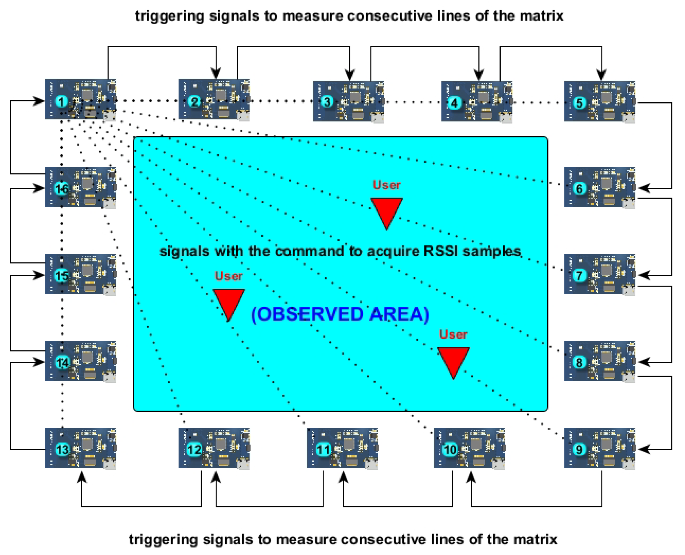
The method of acquiring measurement data at the stage of communication in the PAN (Personal Area Network), as well as an example of transmitter placement, are presented in Figure 1. The graphics show the simplest array of sensors in a standard rectangular room, as well as the formation of the first row of the measurement matrix (dashed lines denote the process of indicator acquisition). After acquiring $n-1$ indicators, where n is the number of radio probes used in the room, the active probe excites the next probe according to the sequence number. The excitation (solid lines with arrows) in the next probe triggers an analogous procedure to that of the preceding probe.

After completing the full cycle, the measurement data frame is collected, and data processing can take place.

2.1.2. Detailed Description

The fundamental, and at the same time the smallest, building block of the RTI system is the radio probe presented in Figure 2. It consists of two 2.4 GHz radio chips, each of which can act as both a transmitter and a receiver. The obverse side of the PCB is occupied by the Bluetooth section made in accordance with the fifth generation of this wireless transmission standard. Figure 2 shows a mosaic of the probe’s electrical connections—the red color of the components constitutes 70% of the structure of the BLE module. The focal point of the circuit is the nRF52832 wireless SoC (System on a Chip), which is a platform allowing the implementation of the BLE protocol on the one hand, and a decision-making unit equipped with an ARM Cortex M4 core and a unit specialized in floating-point calculations on the other. In Figure 2, it is identified by the designator nRF1. An SoC is a complementary hardware solution in the form of a highly integrated chip. It encompasses a range of components such as CPU, digital (e.g., input-output ports, communication buses) and analog (e.g., analog-to-digital converters, RF modules).

Near the microcontroller are the mandatory external components required for proper operation: RTC (a so-called watch quartz resonator characterized by the high accuracy of the offered signal) designated Y1, the main quartz resonator Y2 clocked at 32 MHz, communication with the user via LED indicators designated RGB1, inductances L4 and L5 for the internal DC/DC converter and capacitive filters surrounding the SoC. You can communicate with the chip both wirelessly with the help of PAN (Personal Area Network), i.e., short-range networks, such as Bluetooth or IEEE 802.15.4, and wired via a JTAG interface. According to Figure 2, the right edge is reserved for the antenna path (2.4 GHz ceramic antenna (ANT1)) and feeder with matching circuits. In addition to the built-in ceramic antenna, it is possible to switch the track using a jumper (OMN / DIR) with an external antenna. The connection is realized via the u.FL connector (J1). The surroundings of the antenna track have been completely stripped of the ground (spout) layer, and their boundary edges have been filled with potential equalization points under both sides of the laminate. A 3D visualization of the PCB obverse is presented on the left panel in Figure 3.

The reverse side of the PCB in its entirety (the layer marked in blue) is occupied by a radio chip that allows the use of the IEEE 802.15.4 standard. It comes in the XBee S2C module, which has all the components on a separate laminate. The XBee module is connected to the main PCB with surface solder connections. The metal body shields the chip and, apart from the GPIO, interface or configuration leads, only the u.FL connector for connecting a customized antenna is brought outside. The chip has its API, which can be communicated via a UART serial port. This port is connected to the control unit of the entire device, the nRF52832. A visualization of the reverse PCB is presented on the right panel in Figure 3.

Radio probes can connect directly but do not have enough computing power to share processes between data acquisition, data coordination and pre-processing. In addition, they are not capable of communicating with the local network. The burden of all processes other than taking measurements has been shifted to a specialized unit in the form of a single-chip computer. Together with a touchscreen display, a proprietary BLE expander, an omnidirectional antenna and a case, they constitute a mobile device that guarantees the probes network access, computing power and, in the case of LAN problems, a place to aggregate and archive measurement results (with the help of PAN). The idea of the device is presented in the form of a block diagram in Figure 4.

Transferring the burden of segregation and aggregation of measurements to the central unit also brings energy savings, which, despite the outlay of additional equipment, are achieved by densely covering the building space with an RTI network supporting the control of devices responsible for regulating light, heat, ventilation or air conditioning. Limiting the functions performed by the probes to a minimum led to the maximum sleep time for microcontrollers. The signal from the Bluetooth transmitter is distributed in three stages, each of which is radiated at a different frequency (channels 37, 38 and 39). The probe configuration used and the associated current consumption of the BLE stack are presented in Figure 5.

Each of the three transmissions shown and their associated data maintain the peak current consumption of the Bluetooth LE stack for about 380 µs, making the total time in the order of 1.1 ms. In turn, each of the transmissions is preceded by an approximately 500 µs period of standby and radio re-energization. In total, the largest period of Bluetooth stack activity is spread over less than 2 ms of cycle duration. Taking into account the preferred data transmission interval of 100 ms, this represents only 2% of the idle duration, during which the microcontroller consumes 2 µA of sustained current. Ultimately, this results in an average BLE stack current consumption of 230 µA. If the BLE transmitter is present in the system on its own, the current consumption associated with the scanner’s activity should be added to the result. The value will then increase to 282 µA. If the RTI system operates in Bluetooth 5 + IEEE 802.15.4 mode, one should take into account the consumption associated with the operation of the BLE stack in transmit mode only (230 µA) and the average consumption of the XBee module (1.2 mA), i.e., a total of 1.43 mA. The calculations made above are right for a system built with 32 probes, which represents the most demanding case developed. For systems of smaller size, the current consumption resulting from the operation of the probes will be correspondingly smaller. For the sake of completeness,

Table 1. Energy consumption parameters of the standards of the device.

Operation Mode	Working Time (Days)	Average Power Consumption (mW)	Suggested Current Output of the Power Supply (mA)	Suggested Wattage of the Power Supply (W)
Bluetooth 5	147	30	640	3.2
Bluetooth 5 + IEEE 802.15.4	29	151	1628	8.14

has been drawn up, representing an operating time with a 1000 mA LiPo cell, average power consumption and dedicated power supply with wired power.

To estimate the current consumption of a central processing unit, we use the manufacturer’s technical documentation indicating the suggested current capacity of the power supply and output power. Depending on the single-chip computer used, this can range from 2 to 4 A at 5 V. This makes the power requirement in the range of 10 to 20 watts, which, combined with the probe system, gives a target power of no more than 30 watts at peak. Compared to a traditional incandescent bulb of 60, this represents 25% to 50% of its total power requirements. Compared to the value of occupant presence and location data obtained through the RTI system (regardless of the size of the building), this represents a negligible percentage of the power of the property’s total energy demand. Given the multitude of electrical consumers present in the rooms of modern commercial buildings, electrical savings are derived from the elimination of absentmindedness and mismanagement of resources by the human factor. The reliability of presence verification comes from the fact that the user does not need an electronic device to transmit a radio signature. In combination with the radio ID, on the other hand, the RTI system is also capable of assisting artificial intelligence in cueing the user to adjust the settings of the comfort modules in accordance with their preferences. As a result, it has become possible to deepen the energy-saving effects on a building-wide basis to as much as 20%.

The basic idea of the presented device was to create an access gateway for all the minor modules included in the RTI system. Due to the insufficient bandwidth of the factory network card and the confirmed high unreliability in relation to the application, it was decided to replace the built-in BLE 4.2 with its own Bluetooth 5 adapter. It brought, among other things, such benefits as the ability to use the latest version of BLE and eliminated data bandwidth problems. The SBC’s built-in network adapter shared a hardware resource in the form of an antenna between two wireless data transmission protocols: WiFi and Bluetooth. The separation also made it possible to bring the BLE omnidirectional antenna outside the body of the device. The expander is an SoC nRF52832 connected to the SBC via a serial port. Unlike the probes, its primary task is to provide communication between the probes and the server intended for reconstruction. Structurally, the device differs in that the PCB is surrounded by additional connectors that allow for quick and easy installation in structures similar to the one shown in Figure 4. The central unit was equipped with an operating system from the Linux OS family, and the control panel was created with the help of the Qt Creator environment. The program is called automatically at startup and gives the possibility to save the acquired data to a file, send it to the reconstruction server or view the created background and measurement matrix in real-time.

2.2. The Principle of Measurement

The developed solution involves cyclic measurement of signal strength between at least two devices and then relating the position of the transmitter and receiver to a point on the plane of the room. The measured signal strength is called RSSI and is expressed in decibels referenced to 1 mW (dBm). The property of lossy transmission of a radio wave through the space dividing the devices is used here. This causes significant changes in the amplitude of the signal induced in the receiver antenna and thus gives information about the intersection of the line of sight of the devices. This line of sight will hereafter be referred to as the projection angle. Due to the fact that EM waves are highly absorbed by water, this phenomenon is ideal for the detection of organic obstacles, such as people. To a lesser extent, this method also works well for locating inanimate objects, specially built of metals. The idea presented can be symbolically represented by Figure 6.

The 2.4 GHz ISM (Industrial, Scientific, Medical) band was used as the carrier frequency of the transmitted signal. Signal modulation for BLE and IEEE 802.15.4 is phase keying with Gaussian curve approximation (GFSK). Bluetooth uses frequencies assigned to three channels: 37 (2402 MHz), 38 (2426 MHz) and 39 (2480 MHz). These are frequencies used for detecting and recognizing each other’s devices, broadcasting and other communications involving a one-to-many model. Their location in the band is presented in Figure 7. In the case of IEEE 802.15.4, no overhead is applied to specific transmission channels, and a one-to-one transmission type is used. Detection and determination of the user’s position in the room are carried out by increasing the number of radio probes and placing them around the perimeter of the test zone (usually a wall). Each possible pair of transmitters adds a new projection angle to the model, which resembles a grid filling the two-dimensional model of the test zone. Studies in this field have been performed for three systems of different sizes (8 probes, 16 probes and 32 probes). An example of the distribution of projection angles (grid) is presented in Figure 8. In the illustrative graphics, a 16-probe system was used so as not to reduce the transparency of the presented models. The density of the model grid (and thus the number of devices) should be selected according to the room size. For typical office or utility rooms, a system of 16 probes is sufficient in most cases. For large conference rooms and small warehouses, a system of 32 transmitters is better. The way the probes are arranged is also of great importance. Using Figure 8 as an example, it should be noted that the way the probes are placed at the left-top and right-bottom corners have resulted in zones of insensitivity. Most often, these are areas devoid of projection angles, or the number of angles passing through a given sector does not allow unambiguous determination of the object’s position. For the reasons given above, the transmitters’ placement, and thus, the grid’s form, had to be modeled with a uniform and optimal density for each sector of the room covered by the RTI.

Another factor important to the system’s optimization processes was the height of the ring of transmitters girding the surveyed room. An experimental method found that the system has the highest reactivity when operating at a height from the waist to halfway up a person’s torso. It is due to the fact that at this height, the body is the best obstacle in the path of EM waves (high density of rich-in-water organic matter). Finally, the height at which the antenna of the device was located corresponded to the average value of human height at which this section of the human body falls. The RTI probe system, shown in Figure 9 and Figure 10, was attached at a height of 140 cm. Depending on the mathematical tools used in the system, both directional and omnidirectional antennas are allowed, but the tests performed in both cases created requirements to modify the algorithm responsible for the reconstruction. Tests included configurations such as omnidirectional antennas, omnidirectional antennas with screens on the side of the wall, directional antennas, strip antennas in different orientations, ceramic antennas in different spatial orientations and having and not having a screen. The screen was designed to narrow the radiation area to about 180° horizontally and vertically. In addition, it prevented EM waves from reflecting off the metal structural elements of buildings, which, in some places, detrimentally boosted the measured RSSI value. Figure 9 and Figure 10 show probes with strip antennas mounted on a u.FL connector.

Due to their design, radio probes allow measurements to be made in two ways. The first is to make measurements using only the Bluetooth LE protocol. It boils down to using a data frame both as a data carrier and as a source of sampled signal to acquire the RSSI index. Each packet contains information about the RSSI associated with each possible pair of devices. For systems with up to 16 devices, it is sufficient to use a basic data frame designed for broadcasting. For systems of up to 32 probes, the scan response feature characteristic of BLE technology is used. It allows the scanner to send a request to send a packet with additional information. In this way, the amount of available space for user data can be doubled. It should be noted that the signal is always measured from the first packet. All the software controlling the BLE module was created using the C-embedded language. The structure of the communication package is presented in Figure 11. A data container consisting of 6 reserved bytes of memory for flags (R), 3 bytes of a device identifier (IDx), 16 bytes representing a single row of the background or measurement matrix collected by the device data (RSSIxx) and 6 bytes of storage allocated for the possible extension of the transmitter ID number was inserted into the PDU, which has space for user data (omitting the header).

Such a solution is characterized by a minimal number of packets circulating in the area, and the results from calculations performed in the BLE stack go directly to the central unit. It translates into a high refresh rate of the heat map image. The disadvantage of the solution turned out to be the large outlay of filters and signal averaging mechanisms, whose fluctuations could exceed 10 dBm over a distance of several meters. The second way is simultaneously using the BLE stack and XBee modules (IEEE 802.15.4). The way data are segregated and arranged in the BLE packet (which still serves as a transport layer) does not change. The difference is due to the BLE algorithm’s abandonment of the pointer value calculation favoring IEEE 802.15.4. Both modules communicate with each other via a serial port. The application in the nRF52832’s memory forces certain operations on the XBee modules, which issue commands to each other remotely to perform RSSI measurements. It should be noted that the indicators obtained in this way are very stable over time (despite the lack of environmental changes). The measured signals were characterized by a deviation of 1 dBm up and down over a distance of several meters. The disadvantage of this solution is the API slowing down the execution of operations, resulting in the nRF52832/XBee module 1/XBee module 2/XBee module 1/nRF52832 performing operations in at least tens of milliseconds each time. This translates into a lower refresh rate of the image reconstructed by the RTI. The XBee modules can accept commands in wireless form from the CPU (the use of the proprietary XBee expander is then required (simultaneously with the Bluetooth 5 expander)). It provides increased control over the entire system’s operations but slows it down. Another (most common) method used in the project was to excite each other’s devices after taking a measurement (on the principle of cascade connection). At the moment of excitation, the first module (always initiating operation after a reboot or power failure), after collecting RSSI indicators from all other devices, excites the next one according to the sequence number. After collecting all indicators, the matrix row is updated and exposed for acquisition by the central unit in the form of advertising. It should be noted here that this approach makes it so the individual rows of the matrix do not have to refresh one by one. When a transmission error occurs, the failed RSSI packet is ignored, and its previous results are not overwritten (they are stored for transmission/reception failure). Therefore, despite the failure of a single transmitter, the entire imaging system can continue to perform its functions but with lower accuracy. This makes the system as a whole very fault-tolerant. In the case when the application hangs up on one of the devices, the system is equipped with a mechanism for reinitializing the system. A jam in the system manifested itself through a transmission error in the excitation signal between individual devices. After a certain amount of time (usually a little more than the average time of performing reconstruction), which is always counted down by a timer in probe number 1, the devices resume transmission after the system activity disappears (in this case, no excitation signal is received from the last probe in the queue).

2.3. Toward the Reconstruction

In principle, the tomographic methods are governed by the equation, which states the forward problem

$$J·e=m,$$

(1)

where J is the sensitivity matrix, e is the vector of finite elements of the mesh (reconstructed image) and m is the measurement vector. The sensitivity matrix contains information on the geometry of the system. To illustrate how it is created, let us use an example from Figure 12. It presents a setup of an RTI network with 16 sensors. Each node can transmit and receive a radio wave packet to obtain a network with 120 two-way connections.

The analyzed area can be covered with a pixel mesh. We assume that radio signals between the transmitter and receiver propagate inside the first Fresnel zone, which has the shape of an ellipse. Then we assign weights to every pixel, depending on whether it belongs to the Fresnel zone or not. The general formula is

$$w_{ij}=\frac{1}{\sqrt{d_i}}\left\{\begin{array}{cc}\hfill 1,\hfill & \mathrm{if}{d}_{ij}^1-d_{ij}^2<d_i+\delta \hfill \\ \hfill 0,\hfill & \mathrm{otherwise}\hfill \end{array}\right.$$

where $d_i$ is the distance between two radio sensors, $d_{ij}^1$ and $d_{ij}^2$ are the distances from the center of pixel i to sensor j. Finally, $\delta$ is a parameter describing the width of the ellipse. Thus, points belonging to the Fresnel zone get weight 1 while the outside ones 0.

The measurement vector consists of $N^2$ elements (where N is the total number of RT probes). Each represents the RSSI measurement between two RT probes measured in dB. For example, in Figure 13, a sample measurement vector was rescaled and rearranged to a $N\times N$ matrix. This measurement represents a person standing in the central part of the experimental room.

Interestingly, one can notice the arch-like structure of the measurement matrix, corresponding to the electromagnetic wave weakening by the obstacle. This pattern provides a hint that reconstructions can be obtained with the usage of pattern-sensitive methods, such as convolutional neural networks (CNNs), long short-term memory (LSTM) cells and other computer vision (CV) methods.

In order to obtain the image from the measurement, one has to rearrange Equation (1) in the following way

$$J^{-1}·m=e,$$

(2)

with an inverse sensitivity matrix. Obtaining the inverse, or, usually, a pseudoinverse of J is generally a non-trivial task. This is classically performed with various deterministic methods, such as Gauss–Newton, Tikhonov regularization or Moore–Penrose pseudoinverse, to name a few. These methods, however, are very computationally demanding. If one wants to deploy the solution on some lightweight device, e.g., Raspberry PI, the obtained execution times, and thus the frame rate of the image, might not be satisfying.

This is where ML and DL methods come to the rescue. While neural network training requires vast computational resources, obtaining an inference from a trained model does not. Therefore, solving the inverse tomographic problem with DL has the potential to greatly improve the quality of the images and reduce the computation time simultaneously.

2.4. Data Acquisition

To train deep learning models, a vast amount of data are needed. Gathering lots of real measurements with ground truth is costly and requires hundreds of hours. To overcome this inconvenience, we rely on simulations as training data. As the image reconstruction utilizes the inverse problem, for simulating measurements, we use the forward problem (1), which is computationally easier. It means from the assumed content of the room, we compute the simulated RSSI matrix.

We prepare the simulated dataset in the following steps using the self-developed toolkit in the following steps.

• Preparation of the numerical model of the room. The interior of the room is mathematically represented with a pixel mesh.
• Placement of a human-sized gaussian inclusion into a randomly chosen point from the uniform distribution.
• The computation of the RSSI matrix with the forward problem, which is a simple multiplication of the system’s sensitivity matrix and the room mesh.
• Scaling of the RSSI matrix so its magnitude and characteristics match real measurements.

Points from 2 to 4 were repeated 30,000 times giving us our final simulation dataset for supervised ML. To make it more clear, the X is RSSI vectors, while the Y is values of pixels of the mesh.

2.5. Models

In experimenting with measurements and reconstructions, we have prepared three models relying on various ML techniques. To build and train the networks, we used Tensorflow for the first network and Matlab for the remaining. In all approaches, we used the 1D measurement vector representation as an input with the size of 1024 elements (instead of a 32 × 32 matrix). The output is a corresponding vector with pixels of the image. The first model is a fully connected neural network, the architecture of which is presented in

Table 2. The architecture of the fully connected neural network model.

Layer Type	Shape	Activation
Input	1024	-
Dense	256	ReLU
Dense	512	ReLU
Batch Normalization	-	-
Dense	5329	Sigmoid

.

In this network, we treated the problem as a classification. Therefore, the training data were transformed with a threshold function

$$t_{\xi }\left(x\right)=\left\{\begin{array}{c}\hfill 1,x\ge \xi ,\hfill \\ \hfill 0,x<\xi ,\hfill \end{array}\right.$$

(3)

where we used $\xi =0.5$ in this particular case.

We start with an input layer. Then, there are two fully connected layers with 256 and 512 neurons. Both are activated with the rectified linear unit (ReLU). After these layers, the data are normalized with a batch normalization layer, and they go to the final fully connected output layer with sigmoid activation. The configuration is presented in Table 2.

As a loss function, we naturally picked binary cross-entropy. The training was performed using Adam optimizer, with a standard learning rate of ${10}^{-3}$. The training was set with 100 max epochs, 64 batch size and a 0.2 validation split. An early stopping callback, which measured the dynamics of validation loss, was used.

The training lasted for 56 epochs as the loss function reached convergence and was stopped by the callback. Model evaluation on the test revealed an acceptable dose of overfitting. The final values of the loss were 0.0076 in the training set and 0.0096 in the test set.

The second model utilizes several convolutional layers, which are sensitive to geometric structures present in a measurement. One can approach the problem with convolution in two different paths. First, treat the measurement as a 2D matrix (or even a grayscale image) and look for patterns that carry relevant information on the obstacle’s position, size and shape. This allows the use of 2D convolution and some CV methods as well. On the other hand, one can use a 1D representation of the measurements and apply one-dimensional convolution filters to extract the inclusion characteristics.

We use the latter method in this case, treating our RSSI measurements as vectors with 1024 elements. We have already had some successful trials with the first approach [34]. However, we could not obtain decent results with a single model, and using two-stage neural nets was necessary.

As an input, the network takes a 1024-element measurement vector. Then it passes through a convolution layer with 128 filters of large 24 × 24 size and hyperbolic tangent activation. Using such a steep activation function provides a kind of cut-off and helps to deal with noise, which is present in real-world data. After these convolutions, there are layers for regularization purposes, namely a dropout and batch normalization. Finally, convolutional layers are pooled with global max pooling and passed to a fully connected layer that is the output of the model. The architecture of the model is presented in

Table 3. The architecture of the convolutional model.

Layer Type	Shape	Activation
Input	1024	-
Conv1D	128, 24 × 24	TanH
Dropout	0.05	-
Batch Normalization	-	-
Global Max Pooling	-	-
Dense	5329	ReLU

.

The third network is recurrent and is based on long short-term memory cells. Usually, such networks are used for time series-related tasks, such as the prediction of the next step or classification of the time series. It can be questionable because our data are not related to any time-dependent phenomena, as it is a static measurement data frame. However, generally speaking, LSTM, especially in its bi-directional variant, is extremely sensitive to sequenced structural patterns. The structures seen in Figure 13 conserve their pattern and information in a one-dimensional representation. Therefore, the usage of recurrent techniques is justified, as we deal with structured data in one dimension.

The final model has the least number of layers, as only four are listed in

Table 4. The architecture of the LSTM model.

Layer Type	Shape	Activation
Input	1024	-
Bi-Directional LSTM	2048	TanH
Dropout	0.1	-
Dense	5329	ReLU

. The first is the input layer, which passes data to a bi-directional LSTM layer with 2048 cells and hyperbolic tangent activation. Then, a regularizing dropout layer with 0.1 probability is applied, and a fully connected layer with ReLU activation is an output of the model.

Both networks (CNN and LSTM) were built as regression models. Therefore, their loss function is the well-known mean squared error (MSE)

$$MSE=\frac{1}{N}\sum _{i=1}^N{(y_i-{\widehat{y}}_i)}^2,$$

(4)

with y being the real value and $\widehat{y}$ predicted by a model. In our case, these are ground truth and reconstruction, respectively. For additional monitoring of learning, the root mean squared error (RMSE) was used, which is simply a square root of the above formula. The networks were trained using the Adam optimizer with an adaptive learning rate with an initial value of ${10}^{-3}$. The training went regularly and was characterized by exponential convergence. The training process was terminated by an automatic callback function after 378 iterations for CNN and 342 iterations for LSTM.

The reconstruction time for a single observation took less than 50 ms for each model. The calculations were performed on an Intel^® Core™ i5-8400 2.80 GHz processor, 16 GB of RAM and an NVIDIA GeForce RTX 2070 GPU.

3. Results

This section presents the reconstructions of several measurements we have conducted. The reconstructions were obtained with three different ML models. Naturally, we compare the results to the ground truth.

We have conducted hundreds of measurements during our work and experiments. However, we cannot present all of them for obvious reasons in this paper. Therefore, we randomly picked three measurements and presented their reconstructions. The ground truth was generated manually from the known position of a person in the room. The test subject was an average-sized male, and the test room was a small conference room of approximately 20 square meters.

The results can be seen in Figure 14, Figure 15 and Figure 16. In each figure, there are four panels—ground truth and three reconstructions from our models, fully connected neural network, convolutional neural network and long short-term memory recurrent neural network, respectively. In addition, every visualization has a contour of the room (red line), and the positions of RTI probes (blue dots) marked.

It can be clearly seen that all algorithms precisely retrieve the position of the human in the room. In all three cases, the reconstructed shade is in the same place as in the ground truth (panels a). However, there are differences in the shape of the subject.

The fully connected network gives us the smallest object reconstructions. This can be justified by the classification setup we adopted in this approach. The output image passes through the sigmoid function, which cuts off smaller values of pixels.

It does not happen in regression models (CNN and LSTM), as the inclusions are bigger and sometimes even smeared. What is interesting, different models seem to work better for different inclusion placements. In Figure 14, all models performed more or less the same visually. However, in Figure 15, CNN outperforms the remaining models, both in size and position of inclusion. On the contrary, in Figure 16, the fully connected network performed the worst, while the remaining two achieved much better results.

This brings us to the conclusion that using only one model for the reconstruction might be suboptimal. A better solution would be to determine in which case the model performs better on the given input data and pick the favorable one. On the other hand, one might think of an inspiration from ensemble learning, where a family of models predicts the image, and then some fusion occurs. It can even be the simplest averaging with some initial filtering, up to a more sophisticated data aggregation method.

On the quantitative side, the results of the models computed on the test set data are collected in

Table 5. The metrics of the models on the test set.

Model	SSIM	PSNR
Fully connected NN	0.9712	25.82
CNN	0.9674	23.99
LSTM	0.9724	25.11

. For verification of their performance, two metrics were used. The first is the structural similarity index metric (SSIM), which focuses on the similarity of the spatial distribution of structures in the picture. Moreover, it mimics human perception of the similarity between two images. The other is peak signal-to-noise ratio (PSNR), which is a well-known, standard measure in signal processing.

In general, all models perform pretty well, and their metrics are high. However, it appears that the LSTM model has the best result in SSIM, but the fully connected network achieves the best PSNR value. This means that the LSTM-based network is the best at reconstructing the spatial structure of the image, in other words, which pixels light up. On the other hand, the fully connected model is the best at deciding the intensity of the pixels. As we already mentioned, these results seem complementary and should be merged into one picture to enhance the reconstruction quality even more.

Nevertheless, the obtained results from ML algorithms look far better than those we obtained with the inverse sensitivity matrix. This is because ML-based reconstructions lack artifacts commonly present in the aforementioned deterministic methods. Therefore, an additional, yet minor, advantage of our approach is the lack of necessity of using numerous post-processing algorithms to obtain clean and acceptable imaging.

4. Discussion and Conclusions

This paper presents a novel RTI device with 32 probes and machine learning-based image reconstruction algorithms. The system is designed to be cheap and accessible in terms of its price and energy consumption. The presented device is designed for passive localization in smart buildings and optimal energy management. Precise information about user presence and location can be used to steer various devices, such as window curtains, air conditioning, heating and lights.

The results are greatly satisfying from many perspectives, as the system can visualize a person without additional devices (such as smartphones). First, we could eradicate most of the noise we dealt with in previous versions of the device. It gave us stable and reliable RSSI measurements with a standard deviation of around 1 dBm. Unfortunately, the price to pay for such precision was the time of taking one frame. The frame rate is significantly lowered, and we aim to introduce some improvements to make it bigger.

Secondly, the machine learning models trained on simulated data sets gave very good results on real-world measurements. They proved to be resistant to noisy data from real measurement, which is one of the most important findings of the paper. It shows that our simulations of RTI and reality play along, which is very promising. Collecting data for analysis and training usually takes a lot of effort and cost, which can be avoided. It gives good opportunities to our device, especially given future commercialization, because it makes it easily deployable. A possible deployment would not require hours of data collecting. However, setting up the room geometry, performing simulations and transfer-learning of prepared models on new data can save many problems for a potential user.

To summarize, we successfully tested the new version of the device. From the hardware side, we achieved a stronger and more stable signal with respect to the past versions. On the software side, we trained robust neural networks, which precisely locate a person in the room. This combination presents new quality, and the following progress will be reported in future works.

The presented RTI setup can also be used for various smart home tasks. These are specifically related to some medical problems, such as fall detection, which can also be important in hospital deployments. Adding another ring of probes can give us additional information on the height dimension. Such data would allow for tracking the body position of the person. We shall return to these problems elsewhere.