Embedding-Graph-Neural-Network for Transient NOx Emissions Prediction

Abstract

Recently, Acritical Intelligent (AI) methodologies such as Long and Short-term Memory (LSTM) have been widely considered promising tools for engine performance calibration, especially for engine emission performance prediction and optimization, and Transformer is also gradually applied to sequence prediction. To carry out high-precision engine control and calibration, predicting long time step emission sequences is required. However, LSTM has the problem of gradient disappearance on too long input and output sequences, and Transformer cannot reflect the dynamic features of historic emission information which derives from cycle-by-cycle engine combustion events, which leads to low accuracy and weak algorithm adaptability due to the inherent limitations of the encoder-decoder structure. In this paper, considering the highly nonlinear relation between the multi-dimensional engine operating parameters the engine emission data outputs, an Embedding-Graph-Neural-Network (EGNN) model was developed combined with self-attention mechanism for the adaptive graph generation part of the GNN to capture the relationship between the sequences, improve the ability of predicting long time step sequences, and reduce the number of parameters to simplify network structure. Then, a sensor embedding method was adopted to make the model adapt to the data characteristics of different sensors, so as to reduce the impact of experimental hardware on prediction accuracy. The experimental results show that under the condition of long-time step forecasting, the prediction error of our model decreased by 31.04% on average compared with five other baseline models, which demonstrates the EGNN model can potentially be used in future engine calibration procedures.

1. Introduction

In the last decades, the greenhouse effect has gradually become a global issue [1], and higher thermal efficiency and lower emission output have become the primary goals for the development of modern internal combustion engines. Correspondingly, emission regulations are becoming increasingly stringent to reduce emissions in the transportation section of each country [2,3]. Automotive manufacturers need to meet these regulations under complex transient test conditions, and to minimize vehicle emissions. In fact, there is a significant difference between the steady-state test and transient test of engine emission performance [4]. Steady-state data usually means the average output value of the engine over a period. Due to the low time resolution of conventional emission analyzers, the results of steady-state experiments normally cannot compare with real-time engine performance. Fast response emissions analyzers can collect transient data to measure emissions variations under transient operating conditions such as engine start/stop and acceleration/deceleration. Transient operating conditions normally represent the real engine working conditions, sometimes with an extremely high-resolution ratio. Therefore, as an assessment tool, an accurate engine emission prediction model, which can be applied to evaluate the engine transient emission performance, is critical for engine control and calibration.

In view of the deficiency of online NOx monitoring equipment in practical application, CFD (Computational Fluid Dynamics) simulations [5,6,7] are commonly used to predict NOx emissions and have been applied to optimize the engine control strategies in the past. However, for real-time forecasting demand, CFD is not applicable due to its high computational cost, high calibration requirements, complex structure [8,9,10,11] and poor adaptability to different engines. Considering the high dimensional engine control MAPs and lookup tables which are embedded in the engine ECU system, the number of experiments required is exponential, which leads to excessive cost. Recently, Acritical Intelligent (AI) methodologies have been widely considered as promising tools for engine performance calibration, especially for engine emission performance prediction and optimization. Liu et al. [12] combined a data preprocessing and long and short-term memory (LSTM) model [13] to estimate numerical emission predictions under unsteady conditions with acceptable accuracy. Kiyas et al. [14] modeled combustion efficiency and exhaust emission indexes for a turbocharged engine with an LSTM model. Halil et al. [15] compared a Deep Neural Network (DNN) to a traditional artificial neural network (ANN) [16,17,18] method regarding the emission prediction ability. The results showed that the performance of the DNN model was much better than the traditional ANN model with a lower relative error. However, the above models are only applicable to single time-step emission prediction, and their multi- time-step forecasting performances are limited.

To achieve a high-precision engine control and calibration method, predicting long time step emission sequences is required [19]. Emission prediction can be viewed as a time series forecasting problem and a long sequence time-series forecasting problems. In the last decade, performance degradation has proved to be the major limitation of the LSTM model due to gradient disappearance [20]. On the other hand, the Transformer model [21] has made breakthroughs in sequence events prediction [22,23]. However, both models ignore the interconnection between multivariate time series and cannot capture the information of high frequency variation characteristics. In addition, the quadratic computation process for solving the self-attention mechanism leads to a further limitation of the transformer model when predicting a long sequence [24]. The potential solution for handling the above issue is a graph neural network (GNN) model [25], since it enhances the spatial modeling and spatiotemporal feature extraction ability. GNN is based on the graph convolution structure, which has the possibility to avoid the gradient disappearance problem.

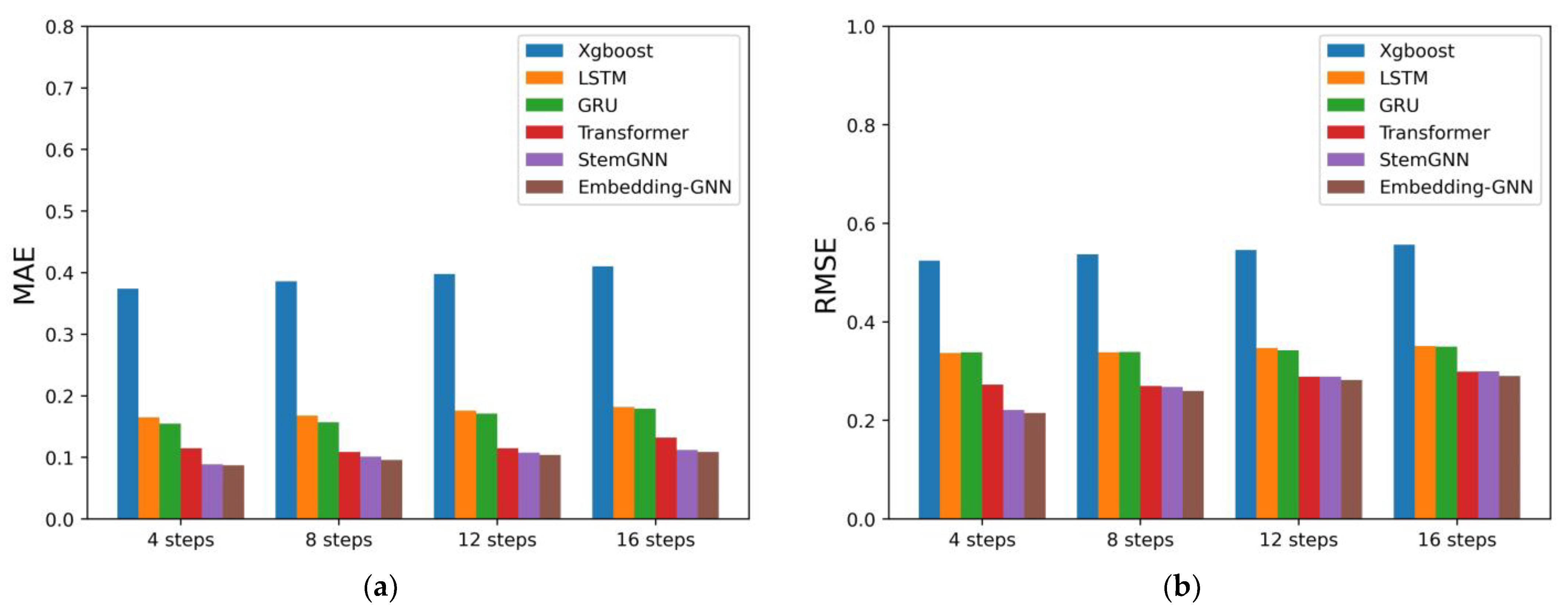
Based on the above analysis, the main purpose of this study was to create a general method for engine NOx emission prediction with high prediction accuracy. We propose a novel graph neural network model based on dimensional embedding algorithm (EGNN), and the performance of this model is and conventional GNN model. The results show that the present EGNN model yields higher accuracy and better performance. A fast emissions analyzer is utilized in this study for data acquisition. Compared with the steady-state emission meter, fast emissions analyzers can obtain more data in a given time period and save the experimental cost.

To achieve such a goal, the main tasks of this work can be described as follows:

(1)

First, attaching a multi-dimensional variable encoding layer to the attention map learning layer. Since there are signal characteristic differences between different sensors such as data accuracy, digital resolution and signal drifting level, an encoder layer is applied to deal with these differences and embed them into the network as a new data feature. In addition, the application of the encoding layer guarantees the EGNN model a better anti-noise performance comparing to other models.

(2)

Second, a sparse attention method is coupled with the self-attention graph generation mechanism to convert the high-dimensional graph relationships into low-dimensional ones, thereby the reduction of model inputs and memory overhead becomes possible [26]. In addition, the proposed attention mechanism provides the ability to accurately predict the long-time step sequence. Compared with the traditional GNN, the self-attention mechanism generates a graph structure automatically, which saves the process of manually finding the relationship between variables.

(3)

To improve the data accuracy, transient emitters are applied in the EGNN model rather than those steady emitters. Hence, the time cost can be significantly reduced when large dataset being processed.

The article is organized as follows. The related work is presented in Section 2. The structure of the proposed method is introduced in Section 3. In Section 4, the basic parameters of the engine, the bench test process and the method of data preprocessing, are described. We compare the proposed method with five other models in Section 5, and the paper is concluded in Section 6.

2. Related Works

In this section, studies related to engine emission prediction based on machine learning methods in the past 3 years are summarized for better understanding the background of the present study.

Mohammad et al. [27] utilized three machine learning methods to predict engine emissions, namely LSTM, ANN and random forest, and better results were achieved compared to traditional emission predicting methods. Aran et al. [28] used principal component analysis (PCA) in an emission forecasting model to reduce the number of input variables. The results showed that the predicting performance of the model can be improved in a condition in which the computational budget is limited. On the other hand, Armin et al. [29] studied the effect of different input variables on an SVM model under four different engine steady operating conditions. It was found that a model with multiple input variables yielded higher accuracy. Ma et al. [30] combined ANN and a particle swarm optimization algorithm, and the engine fuel consumption and emission performance were well predicted. The above research mainly focused on steady-state conditions, and the methods used were mainly traditional ANN and machine learning models. Our paper considers both the engine steady-state and transient-state conditions.

Fang et al. [31] applied a fast response emission analyzer in their study. The results showed that a transient model could be developed and the prediction of transient NOx emission became possible. To reduce the dimension of input variables in the emission predicating model, Nick et al. [32] tested two filtering approaches, a p-value test method, and a Pearson correlation coefficient method. Yu et al. [33] combined LSTM and filtering methods to predict NOx emissions under engine transient conditions. Compared with the studies listed in the literature [31,32,33], the major novelty of our paper is that for the first time, the possibility of modeling long-term emission sequence with fewer variables is demonstrated and verified, and the accuracy of the model developed in this work is significantly improved.

3. Research Methods

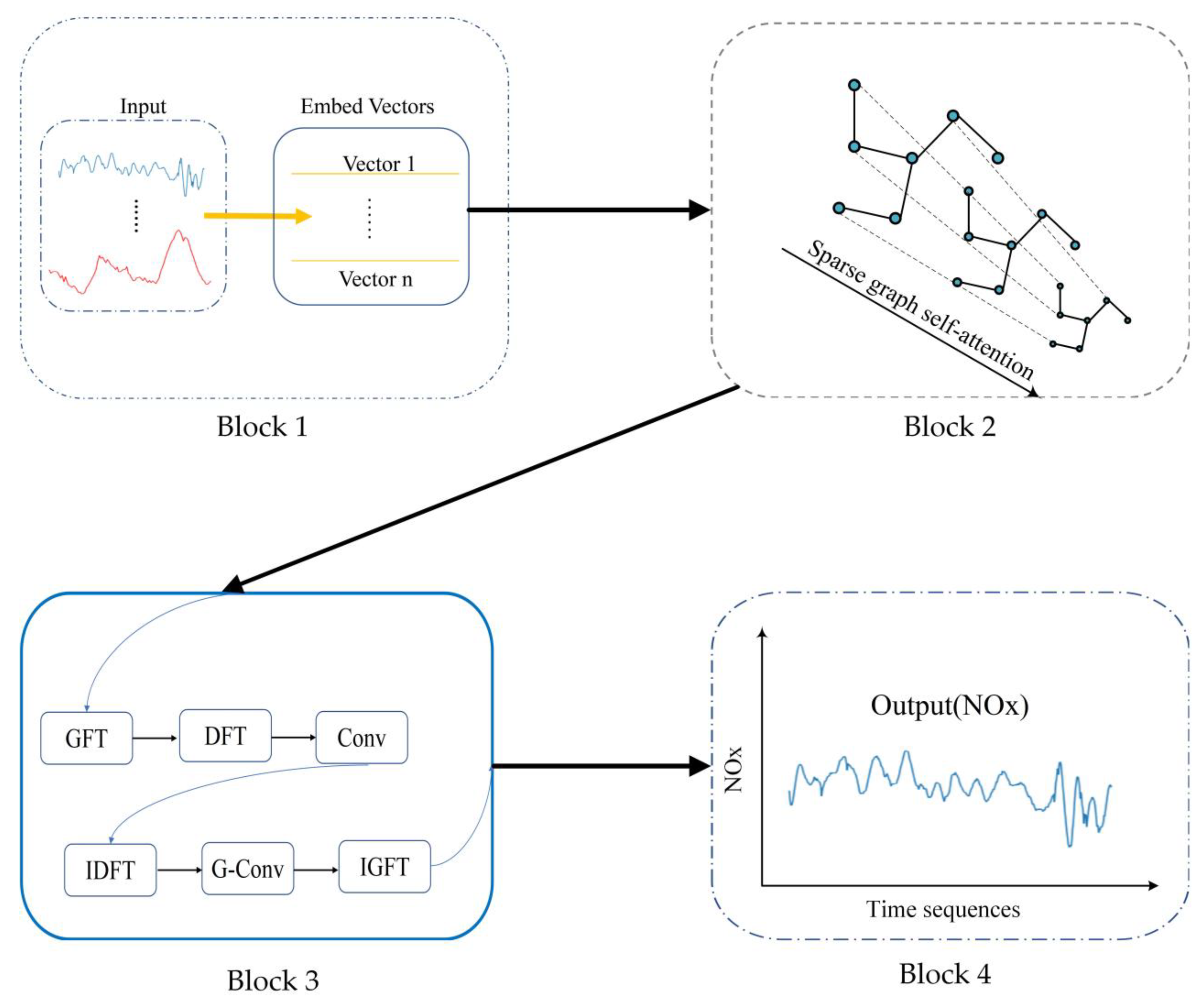
Figure 1 is a schematic diagram of our proposed structure, and involves four main blocks introduced in the following sections.

Multidimensional Variable Embedding (Section 3.2): process the variables by the embedding method to learn the unique characteristics of sensors.

Sparse graph self-attention mechanism (Section 3.3): develop a graph structure adaptively based on the improved self-graph-attention mechanism for the neural network.

Graph neural network based on Fourier transform (Section 3.4): adopt spectrogram GNN to capture the relationship in the graph structure and complete the establishment of the emission prediction model.

Output block (Section 3.4): output the prediction result of NOx.

3.1. Problem Definition

The NOx emission prediction is based on the time series of historical emission information to estimate the emission values in the future, which means the emission values of time $t+\Delta t$ can be predicted at time t, where $\Delta t$ denotes time interval between two points. To capture the relationship between multivariate variables and NOx, the data structure, multivariate graph shown in Figure 2 is adopted.

We define the multivariate variables model as a graph $G=(X,A)$, where X = {x₁, x₂, ..., x_N} is a finite set of N nodes that represents multivariate variables and x_i$\in {ℝ}^{m\times T}$ where T is the timestamp and m is the embedding dimension, which will beis explained in the Section 3.3. $A^{N\times N}$ represents the adjacency matrix of graph G.

With the input values of previous L time steps X_t−l, X_t−l+1, ..., X_t, our target is to predict the K time step values of the NOx emission. The prediction can be denoted by X_t+1, X_t+2, ..., X_t+h, and inferred by the deep learning model Y (G, X_t−l, X_t−l+1, ..., X_t).

3.2. Multidimensional Variable Embedding

Multidimensional variables represent multiple characteristic inputs to the model. Various sensors have their own unique characteristics in different stages and environments. At the same time, their initial noise values are different. To reduce the influence of hardware on the model’s prediction performance, we utilized an encoding method to generate feature vectors for multidimensional variables. Compared with the positional encoding in Transformer [21], the embedding vectors provided to the input variables are learnable.

Figure 3 is a schematic diagram of encoding. The representation method for embedding vector is as follows:

$$V_i=\left({\omega }_{i1},{\omega }_{i2},\dots ,{\omega }_{id}\right) \mathrm{for} i \in \{1,2,\dots ,N\},d\in N^{*}$$

(1)

where N is the number of the variables and N* is positive integer set.

3.3. Sparse Graph Self-Attention Mechanism

3.3.1. Sparse Self-Attention Mechanism

In the Transformer [26], the self-attention calculates the dot product of the i-th query as follows:

$$ST(q_i,\mathit{K},\mathit{V})=(q_i{\mathit{K}}^T/\sqrt{d})\mathit{V}$$

(2)

where d is the model’s input dimension, q_i is the i-th row of Q, and Q, K, V$\in {ℝ}^{L\times d}$. L is the input sequence length.

In the self-attention mechanism, according to the Formula (2), the probability distribution of Q and K is as follows:

$$p(k_j|q_i)=\mathrm{K}(q_i,k_j)/{\displaystyle \sum _l\mathrm{K}(q_i,k_l)}$$

(3)

$\mathrm{K}(q_i,k_j)$ is the asymmetric exponential kernel $\exp (q_i{k_j}^{\mathrm{T}}/\sqrt{d})$, $q_i,k_j$ representing column i of Q matrix and column j of K matrix, respectively.

We define a uniform distribution as $x(k_j|q_i)=1/L$. When the matrix probability distribution of Q and K approximates a uniform distribution, then, for the overall self-attention mechanism, the weight is approximated to a random input, which means the neural network loses its function. Therefore, we adopted the MMD method (Maximum Mean Discrepancy) shown in Formula (5) to measure the similarity between parameter weight distribution and uniform distribution.

$$d_k^2(p,q)={\parallel E_{x~p}[\mathsf{\Phi }(x)]-E_{x~q}[\mathsf{\Phi }(x)]\parallel }_{\mathrm{H}k}^2$$

(4)

For the convenience of calculation, Formula (4) is transformed into the following form, and the linear kernel function is used for mapping:

$$\begin{array}{c}U(p,q)=\frac{1}{L^2}(e^{\frac{q_i{k}_j^{\mathrm{T}}}{\sqrt{d}}}{\displaystyle {\sum }_{a=1}^L{e}^{\frac{q_i{k}_a^{\mathrm{T}}}{\sqrt{d}}}}\\ +{\displaystyle {\sum }_{a=1}^L(\frac{1}{L^2}}-2e^{\frac{q_i{k}_a^{\mathrm{T}}}{\sqrt{d}}}))\end{array}$$

(5)

Multiply both sides of the above equation by L² and drop the constant to get the Formula (6):

$$U(p,q)=(e^{\frac{q_i{k}_j^{\mathrm{T}}}{\sqrt{d}}}-2){\displaystyle {\sum }_{a=1}^L{e}^{\frac{q_i{k}_a^{\mathrm{T}}}{\sqrt{d}}}}$$

(6)

Following the inference in the informer [28], which is $\ln {\displaystyle {\sum }_{a=1}^L{e}^{\frac{q_i{k}_a^{\mathrm{T}}}{\sqrt{d}}}}\approx \max (\frac{q_i{k}_a^{\mathrm{T}}}{\sqrt{d}})$, the Formula (6) can be rewritten as the following form:

$$U(p,q)=e^{\frac{q_i{k}_j^{\mathrm{T}}}{\sqrt{d}}}\cdot \underset{j}{\max }(e^{\frac{q_i{k}_a^{\mathrm{T}}}{\sqrt{d}}})-2{\displaystyle {\sum }_{a=1}^n{e}^{\frac{q_i{k}_a^{\mathrm{T}}}{\sqrt{d}}}}$$

(7)

By Formula (7), dot product pairs with higher attention weights are screened out to make the size of learned graph smaller, with the depth of the model reduced concerning parameters memory consumption as shown in Figure 4. Therefore, the matrix Q is transformed into the sparse special matrix in Formula (8). The hyperparameter s is set that indicates the Top-s product pairs are selected as the input of the next layer.

$$Q^{\ast }=sam(Q|u(p,q))$$

(8)

where sam(.) is the function that samples the q in top-s product pairs to generate the Q*$\in {ℝ}^{s\times d}$.

3.3.2. Graph Construction

Simple GNN-based methods require a graph structure when modeling engine multidimensional parameters. The graph structure can be constructed by physical knowledge or experience, which can be difficult to build because of the nonlinear relationship among the parameters of the engine. To adapt to different engines, we utilize the sparse self-attention mechanism to automatically learn the potential correlations between multiple engine parameters as shown in Formula (9):

$$G=\mathit{Softmax}(\mathit{relu}(K{Q}^{\ast }/\sqrt{d})V)$$

(9)

where Q* is the sparse spatial matrix generated in Formula (8), relu function is chosen as the activation function, and Softmax is adopted to normalize the generated graph.

In this way, the model builds a graph structure of its own parameters in a data-driven manner.

3.4. Graph Neural Network Based on Fourier Transform

Most time series research has focused on the time-domain correlation between multi-dimensional variables, while ignoring the intrinsic relationship between the parameters in the frequency domain. Considering the high-frequency variation of parameters caused by high engine speed, we attempted to use an improved spectrogram neural network to establish an engine emission prediction model by combining the graph generated in the Block 2 of Figure 1. The improved spectrogram neural network Block is displayed in the block 3 of Figure 1.

To combine the sensor embedding vectors v_i with the neural network, we improved the overall calculation flow. First, our graph generator incorporates v_i and to do this, we compute the graph attention as follows:

$$z_i{}^{(t)}=v_i+x_i{}^{(t)}$$

(10)

$$h(i,j)=Gelu(w_q{z}_i\cdot w_k{z}_j)$$

(11)

$${\alpha }_{i,j}=\frac{\exp (h(i,j))}{{\displaystyle \sum \exp (h(i,k))}}$$

(12)

where Formula (10) combines the input features and embedding vectors, and Gelu is used as the nonlinear activation to calculate the attention coefficient in Formula (11). Softmax function normalizes the attention coefficients in Formula (12).

The generated emission graph is transformed into a spectral matrix by Graph Fourier Transform (GFT), which maps the input graph to an orthonormal space based on the normalized graph Laplacian. The normalized graph Laplacian Lap is shown in Formula (13):

$$Lap=I-D^{-0.5}G{D}^{-0.5}$$

(13)

where I is the identity matrix, D is a degree matrix and G is the graph generated in Formula (9).

In Formula (14), the Lap can be spectrally decomposed, the matrix composed of its eigenvectors is U, and A is the eigenvalue matrix.

$$Lap=UA{U}^{\mathrm{T}}$$

(14)

Therefore, GFT and Inverse Graph Fourier Transform (IGFT) can be calculated as shown in Formulas (15) and (16).

$$F(X)=U^{\mathrm{T}}X=\widehat{X}$$

(15)

$$F^{-1}(\widehat{X})=U^{\mathrm{T}}\widehat{X}$$

(16)

After the operation, the multi-dimensional sensor variables become independent of each other. Then, by the Discrete Fourier transform (DFT) operation, variables for the engine are transformed into the frequency domain, which can capture feature information under the Gated Linear Units (GLU) layers’ transform and the convolution layer. Inverse Discrete Fourier Transform (IDFT) brings the variables back to the time domain. Finally, we use the graph convolution in Formula (17) and IGFT to generate the final output.

$$\mathit{G}-\mathit{conv}={\displaystyle \sum _{k=0}^K{\theta }_k}{(UA{U}^{\mathrm{T}})}^k$$

(17)

where ${\theta }_k$ is the weight of the k-hop neighbor.

4. Engine Bench and Data Preparation

To measure the prediction performance of EGNN, we conducted multiple sets of experiments on an engine with model JLB-4G14TB, and obtained a dataset called EDT containing 140,000 sample points.

4.1. Test Bench

The research was based on a four-cylinder, four-stroke, gasoline engine, whose specifications are presented in

Table 1. Engine specifications Engine specifications.

Engine Parameters	Values
Intake mode	Turbocharger
Number of cylinders	4
Maximum power rotational speed	5200 rpm
Maximum torque rotational speed	1600–4000 rpm
Displacement	1.4 L
Valves per cylinder	4
Valve system	DOHC
Maximum power	104 kW
Maximum torque	235 N.m
Cylinder head material	Aluminum alloy

. A schematic diagram of the test bench is shown in Figure 5.

In the test bench, the intake pressure and exhaust-gas pressure were measured by a CYYZ11A pressure transmitter. The intake temperature and the exhaust-gas temperature were measured by PT100 and a thermocouple temperature sensor, respectively. The torque was controlled by a motor which connected the CompactRIO control system. The NOx emission was measured by a Cambustion CLD 500 transient emission analyzer. All sensors were connected to the PXI hardware platform for data acquisition. The model and measurement accuracy of the experimental equipment are shown in

Table 2. Measuring devices of the engine test bench.

Equipment Name	Type	Precision
Thermocouple temperature sensor	WRN-230	±0.5 °C
Air intake temperature sensor	PT100	±0.15 °C
Photoelectric encoder	A-CHA	±0.1°
Transient emission analyzer	CLD 500	NOx:1 ppm
Pressure Transmitter	CYYZ11A	±0.1% FS
Oxygen Sensor	LSU4.9	±1% FS

.

4.2. Work Conditions

In the experiments, engine load was changed from 6 to 100% full load in 2 to 20% intervals by controlling the dynamometer. At the beginning, the speed was controlled at 800 r/min for ten minutes to warm up the lubricating oil. After that, the engine started to gradually accelerate from idle speed to 3500 r/min. During the period, rapid deceleration and rapid acceleration were randomly performed to simulate braking and random acceleration in real road driving conditions. To ensure the amount of data under steady-state conditions, we sampled at intervals of 250 r/min in the speed range from 1000 rpm to 3000 rpm. The scanning time of each interval was not more than 15 s. In addition, we scanned different speeds at the same load condition. The load variation range was 6 to 50%, while the speed range was 1000 rpm to 3000 rpm. The data were collected using the crankshaft angle as a trigger and data collecting was triggered every 180° turn.

4.3. Data Preparation

The data were filtered using the Complete Ensemble Empirical Mode Decomposition with Adaptive Noise method (CEEMDAN) [34]. CEEMDAN makes up for the shortcomings of the EMD method and often be used for high-frequency filtering processing of nonlinear signals. When generating each IMF (Intrinsic Mode Function), white noise is added to reduce the modal aliasing of the EMD decomposition, thereby reducing the reconstruction error.

The partial results of filtering for variables are shown in Figure 6 and Figure 7. The intake air pressure was calculated by using the relative pressure.

The magnitude difference between each feature parameter was too large, which affected the gradient update of network learning and reduced the prediction accuracy, so we adopted the z-score method to standardize the data, as shown in Formula (18):

$$x_z=\frac{x-\overline{x}}{S}$$

(18)

where S is Standard deviation of one-dimensional data and $\overline{x}$ is mean value of the dimensional data.

5. Results and Discussion

5.1. Setting of the Experiments

We set the experiments on the dataset EDT, which is divided into training dataset, valid dataset, and testing dataset at a ratio of 7:2:1. The length of input sequence was set from 4 to 16 to evaluate the long sequence prediction ability of the network. As is shown in Figure 8, the training dataset included data collected from steady-state conditions and smooth acceleration and deceleration conditions. In Figure 9, the testing dataset consisted of a series of data which collected under engine rapidly changing conditions, such as sudden deceleration and rapid acceleration.

The experiments were conducted in the operating system Ubuntu 20.01 with AMD Core R9 CPU (12 core 3.8 GHz),16 GB RAM memory and Nvidia GPU 3070. EGNN was implemented in Pytorch 1.7. In the experiments, we set the batch-size as 64 for training, validating, and testing. The optimizer we choose was the Adam optimizer that optimizes the parameters of the network to minimize the loss.

5.2. Baseline Models

The EGNN was compared with the following five models.

Xgboost [35]: Xgboost, which is a traditional machine learning model for processing sequences.

LSTM [13]: A model based on RNN widely used in deep learning.

GRU [36]: Another model changed from RNN that is applied on natural language processing.

Transformer [21]: Encoder-decoder architecture and the self-attention mechanism is firstapplied on it.

StemGNN [37]: StemGNN is a spatial-temporal GNN and based on graph structure automatically generated and attention mechanism, which can effectively mine the relationship between dynamic spatiotemporal features for time series prediction.

5.3. Performance Evaluation

Accuracy is a very important metric to measure the quality of NOx prediction models. At the same time, accurate prediction plays the important role in the engine control and calibration.

The mean absolute error (MAE), root mean square error (RMSE), precision and the coefficient of determination (R²) were used to evaluate the performance of our model on the EDT dataset. These metrics are represented by the Formulas (19)–(23), where $y$ represents the true value, $\widehat{y}$ represents the predicted value of the model. n is the number of samples.

$$precison=\frac{1}{n}{\displaystyle \sum (1-\frac{|y_i-{\widehat{y}}_i|}{y_i})}$$

(19)

$$RMSE=\sqrt{\frac{1}{n}{\displaystyle \sum {(y_i-{\widehat{y}}_i)}^2}}$$

(20)

$$MAE=\frac{1}{n}{\displaystyle \sum |y_i-{\widehat{y}}_i|}$$

(21)

$$R^2=\frac{(n{\displaystyle \sum y_i}{\widehat{y}}_i+{\displaystyle \sum y_i}{\displaystyle \sum {\widehat{y}}_i})}{[n{{\displaystyle \sum y_i}}^2-({\displaystyle \sum y_i{)}^2}][n{{\displaystyle \sum {\widehat{y}}_i}}^2-({\displaystyle \sum {\widehat{y}}_i{)}^2}]}$$

(22)

$$R=\sqrt{R^2}$$

(23)

5.4. Comparison of Graph Attention Mechanism Results

To investigate the validity of our proposed graph attention method, we performed a case study on two models.

Figure 10 and Figure 11 show the result of graph attention mechanism for StemGNN and EGNN respectively. The data in each grid in the figure indicates the importance of the abscissa to the ordinate. For the completeness of the diagram, we performed attention score calculations for each variable and normalized by Formula (12). After normalization by Formula (13), each value shows the proportion of the influence of the variable on another variable, so the attention scores of the two graph neural networks can be compared.

The variables are listed in

Table 3. Implications of Variables in Figure 10 and Figure 11.

Variable Abbreviation	Implication
Angle	Crankshaft angle
Tin	Air intake temperature
Tout	Exhaust temperature
Pin	Air intake pressure
Pout	Exhaust pressure
Lambda	Equivalence ratio
Fire	Ignition angle
Rpm	Revolutions per minute
Throttle	Throttle valve percentage
NOx	Emissions

. The StemGNN’s attention for NOx mainly focuses on intake temperature, and the attention values of other variables are very low, less than 0.04 while EGNN has a wider attention distribution for NOx where crankshaft angle, exhaust pressure, equivalence ratio, ignition angle and rotational speed have higher attention values. At the same time, crankshaft angle, exhaust pressure, equivalence ratio, ignition angle and rotational speed have a significant impact on emission values according to the emission characteristics of the engine. Therefore, our model not only obtains an outstanding forecasting performance, but also shows an advantage of interpretability.

5.5. Prediction Results Analysis

In this section, we compare EGNN with the other five baseline methods based on the source dataset.

Figure 12 shows the predictions of the baseline models and EGNN under the R evaluation method whose horizontal and vertical coordinates corresponding to true values and the model prediction results. At the same time, the linear fitting function of the true values and predicted values are also shown in Figure 12. The closer the linear function slope is to 1, the higher accuracy the model. The regression slopes were found to be 0.4166, 0.7553, 0.6963, 0.9802, 0.9900, 0.9933 for the six models, and EGNN had the highest slope, which means the best prediction ability. It was shown that the results of Xgboost, LSTM and GRU were more discrete compared to the Y = X function with the results of Transformer, StemGNN and EGNN. Traditional machine learning performed badly on our large sample datasets. Under the R index, StemGNN and Transformer were slightly worse than EGNN in single-step predictability, about 1.2% and 0.3%.

As shown in Figure 13, EGNN achieved a good single time step prediction result. We selected the real values of random dynamic operating points and used six models to predict value for fitting. The predicted time step was one. It can be concluded that EGNN has a good prediction effect on the dataset even if under the random variation of speed and load and intensive changes in working conditions. When the engine operating conditions change rapidly, the first three models have extensive prediction distortion, and cannot accurately predict the change trend of the target value. Among them, although Xgboost can capture the change trend of emissions, it has a large deviation from the target value. Compared with the actual value, the prediction results of LSTM and GRU have obvious phase differences, which may be caused by the insufficient learning ability of RNN structure. The precisions of models are shown in

Table 4. Single time step prediction results of six models.

Metrics	Baseline Methods
	Xgboost	LSTM	GRU	Transformer	StemGNN	EGNN
R	0.743	0.878	0.875	0.983	0.993	0.995
R2	0.553	0.771	0.741	0.968	0.985	0.991
Precision (%)	65.5	86.1	84.1	96.4	96.5	97.3
Linear slope	0.4166	0.7508	0.7236	0.9704	0.9900	0.9933

. It is obvious that our method has the best precision at 97.3%, improving by 49.0, 13.0, 15.7, 0.6 and 0.6%, respectively, compared to the other five models. Comparing Figure 13d,f, the Transformer has a large error in some conditions while EGNN does not.

We used an emission sequence containing 24 time steps to predict the emission at different prediction length, including 4, 8, 12 and 16 time steps of NOx emission. From

Table 5. Prediction results of different time steps based on EGNN and the other five baseline models.

Time Steps		Baseline Methods
	Metrics	Xgboost	LSTM	GRU	Transformer	StemGNN	EGNN
4	MAE (ppm)	41.09	17.31	17.03	9.066	7.016	5.718
	RMSE (ppm2)	98.21	50.24	49.80	22.41	18.14	15.68
8	MAE (ppm)	47.60	18.02	17.75	7.646	7.085	6.356
	RMSE (ppm2)	105.53	51.67	50.84	20.56	19.75	18.66
12	MAE (ppm)	50.19	18.76	18.99	8.105	7.343	7.166
	RMSE (ppm2)	111.71	52.16	52.71	21.73	21.73	20.64
16	MAE (ppm)	56.84	18.45	19.58	11.12	9.436	7.842
	RMSE (ppm2)	118.50	52.19	53.95	26.31	26.49	23.55

, it can be observed that: (1) our proposed model EGNN greatly improved prediction performance on the EDT dataset, and as the time step increased, the prediction error increased gradually and smoothly, which demonstrates the proposed sparse graph attention has great effects on enhancing the prediction capacity in the long time step emission forecast problem. (2) EGNN was superior to the GNN model and StemGNN at all tested time steps, which means the sparse graph self-attention mechanism can better mine nonlinear relationships among multi-variables. (3) The EGNN model shows significantly better ability and prediction results than recurrent neural networks such as LSTM and GRU. The proposed model had an RMSE decrease of 36.2% (at four steps), 23.1% (at eight steps), 18.7% (at twelve steps), and 17.3% (at sixteen steps). This indicates the graph structure had better prediction capacity than the RNN-based models. (4) Compared with Transformer based on encoder-decoder structure and self-attention mechanism, the EGNN also showed better prediction results.

Under the MAE and RMSE index, the prediction performance of our model was better than that of Transformer. As is shown in Figure 14, the advantages of EGNN are still obvious under the normalized MAE and RMSE evaluation methods, under the normalized MAE and RMSE evaluation methods.

From Figure 15, showing the boxplot of prediction errors, it is easy to see that EGNN generates less higher prediction errors, which are marked as outliers in the plot, compared to the other five models. The greatest deviation of the predictions of the first three models close to 500 ppm. The deviations of the latter three were smaller. However, compared with EGNN, the prediction stability of the Transformer wasworse, which is reflected in the larger number of deviation points of Transformer. It means our model has better stability. Combining Figure 15 and Table 5, we can observe that whether under a single time step or a longer time step, EGNN has better predictive ability.

6. Conclusions

We propose a neural network model composed of variable embedding, sparse graph attention and an EGNN block based on Fourier transform. In the present model, both steady-state and transient conditions were considered, and input variables were identified and utilized for improving the model performance. Several insightful results were achieved as follows:

(1)

Based on the feature embedding of Transformer, the Multidimensional Variable Embedding was developed. By assuming that each variable is a node, multidimensional variables was converted into a graph structure. Through the sparse self-attention mechanism technique, the conventional GNN model was optimized to achieve a better ability to capture interrelationships between variables.

(2)

The proposed graph neural network in this study provides a new route for effectively dealing with multi-dimensional variable correlation, high frequency variations and nonlinear NOx concentration time series. Compared with StemGNN, EGNN can focus on more variables in the calculation of correlation weights. Five of these variables received high weight scores in EGNN while StemGNN mainly focused on two variables. This suggests that EGNN can capture deeper interrelationships between variables.

(3)

Comparing the R2 value of EGNN to other typical machine learning-based NOx predicting methodologies such as Xgboost, LSTM, GRU, the R2 value of EGNN increased by 79.2, 28.5, and 33.8%, respectively, under the single timestep. However, the R2 of EGNN only increased by 2.3% and 0.6% compared to Transformer and StemGNN.

(4)

On the other hand, the advantage of EGNN was demonstrated when the index of RSME was analyzed. Comparing the RSME of EGNN with Transformer and Stem GNN, significant decreases of 21.4% and 8.8% could be achieved, which shows the unique long timestep prediction ability of the model developed in this study.

(5)

Increasingly stringent emission requirements generate a huge challenge for automotive engines. Being able to accurately predict the future emission values of the engine plays a key role in engine control. EGNN provides a possible route to reduce the cost of engine production and calibration processes, and provides good predictive support for engine control in the future.

The future research goal is to use different engines to study the transfer learning effect of the emission prediction network model to improve generalization.