On the Optimal Shape and Efficiency Improvement of Fin Heat Sinks

Abstract

In this paper, we analyze the values of the entropic efficiency of longitudinal fins by investigating the coupling between the function describing the fin profile and the corresponding steady-state temperature distribution along the fin. By starting from different boundary conditions, we look at the distribution temperature maximizing the efficiency of the fin. From this temperature distribution and by requesting that the fin must comply with natural physical constraints, such as the maximum fin thickness, we obtain an optimal profile for a purely convective fin and a convecting–radiating fin. For different boundary conditions and for a maximum fin thickness equal to four (in dimensionless units), both the profiles are increasing starting from the fin base until they reach the maximum value and then decrease to zero at the tip. Analytic and numerical results, together with different plots, are presented.

1. Introduction

Longitudinal fins are an effective and well-established means of increasing the heat transfer from a given surface or device to the environment. Practical applications of fins are numerous, ranging from low scales, such as cooling of electronic components, to large scales, such as heat control of heat in heat exchanger tubes or rejection devices for space vehicles (see e.g., the book [1]). There are many types of heat exchangers, reflecting the different means of exchanging heat. Additionally, for specific applications, the use of fins exploiting combined-mode energy transfer are necessary and the interaction of these modes must be analyzed [2]. The potential dependence of the various heat transfer modes on the temperature gives further complexity to the physical models that can result in nonlinear differential equations and usually numerical methods are required to describe properly the behavior of the fins under different conditions.

In this paper, we consider a fin dissipating heat both by convection and radiation mechanisms. The model, described for example by Kraus et al. [1] and Nguyen and Aziz [3], has been extensively investigated by Bochicchio et al. [4] and Giorgi and Zullo [5]. In [6] the authors of this paper introduced a novel indicator for the effectiveness of longitudinal, convecting–radiating fins to dissipate heat: this new indicator measures the dissipation, through entropy rates, of the steady state of the fin with respect to the same dissipation of an ideal fin with the highest dissipation possible. Clearly, the closest the real fin is to the ideal one, the higher will be the corresponding efficiency. A comparison with respect to the classical definition of efficiency for the fins is also discussed in [6]. The distribution of the temperature along the fin at the steady state is coupled with the function describing the profile of the longitudinal fin: the effect of changing the fin profile can result in very different temperature distributions, also by keeping the same boundary conditions. In turns, the temperature distributions and the boundary conditions determine the values of efficiency. How the variation of the temperature, of the boundary conditions and of the many thermodynamic parameters describing the system affect the values of the efficiency is an old problem considered, under many point of view, by many authors (see e.g., Kraus et al. [1], Nguyen and Aziz [3], Mosayebidorcheh et al. [7], Mao et al. [8], Gardner [9]). Here, we propose an analysis of the definition of the entropy given in [6] and of the role that the fin profile plays in determining an effective way to dissipate heat. Indeed, it is known that to different fin profiles there correspond different efficiencies of the fin to remove the heat. In [1] Kraus and Aziz give the efficiency of longitudinal fins corresponding to rectangular, triangular and parabolic profiles. These are also the profiles analyzed in the original work of Gardner [9]. Since then, many papers have appeared regarding the efficiency of fins with suitable profiles. Nguyen and Aziz [3] studied the performance of fins with rectangular, triangular, trapezoidal and parabolic profiles at different values of the Biot number Bi. Marck et al. [10] analyzed the problem from a mathematical point of view, by imposing constraints on the volume or perimeter of the fin and giving non-existence results for both the problems. An overview of the performance of finned tubes with fins of different profiles is given by the review of Basavarajappa et al. [11]. Another review, highlighting the role of geometrical dimensions, dimensionless numbers, and fin location on the performance of the fin, especially applied to latent heat thermal energy storage systems, is given by Abdulateef et al. [12]. The role of radiation combined with the suitable fin profile is analyzed, by a numerical point of view, by Cuce and Cuce [13].

We will consider separately a purely convective fin and a more general convective-radiating fin. The analysis is conducted both by starting from the definition of efficiency as given in [6] and from the classical definition of efficiency. One of the novelties introduced in this work is about the application of the differential equation coupling the distribution temperature and the fin profile: as far as we know, this equation has been used to obtain the temperature distribution for specific fin profile, such as the rectangular, triangular or parabolic. We capsize the point of view: we specify the temperature distribution that improves the performance of the fin and then look at the differential equation as the one satisfied by the fin profile function.

The work is organized as follows: in Section 2, we introduce the physical model and the corresponding boundary conditions. In Section 3, we give the definition of the entropic efficiency, as given in [6]. In Section 4, we analyze the simplest case: the case of a purely convective fin. We divided the section in three sub-sections: after an introductory part illustrating the proposed methodology, in Section 4.1, we consider a fin with a tip at the temperature of the fluid adjacent to the fin, whereas in Section 4.2, a fin with an insulated tip. In Section 4.3, we analyzed the problem of the optimization starting from the classical definition of efficiency. A table summarizing the findings is also given. In Section 5, we consider a convecting–radiating fin: for simplicity we consider the case of a fin with a tip at a temperature equal to that of the fluid. In Section 6, we analyze our results trying to underline the main findings and to elucidate, both from a physical and a mathematical point of view, the conclusions obtained. In Section 8, we discuss some possible applications of our findings. Finally, in the Conclusions, we try to obtain a systematic view of our work and place it within the context: if it is true that there are many physical and mathematical variables involved in the description of the optimization process, we maintain that the preliminary results here presented constitute a concrete basis for further improvements in this area of research.

Numerical and analytic methods are used and discussed also with plots. A further discussion of the results will be given with some remarks about the plausibility of the solutions obtained.

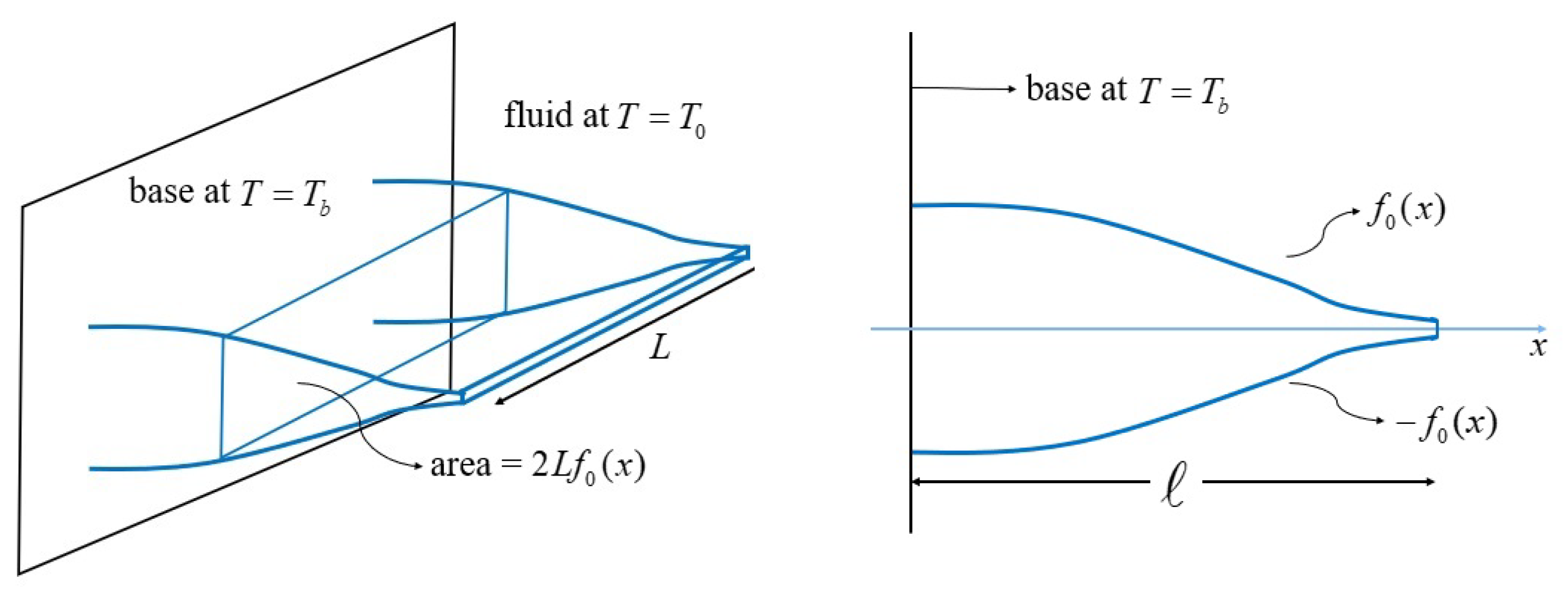
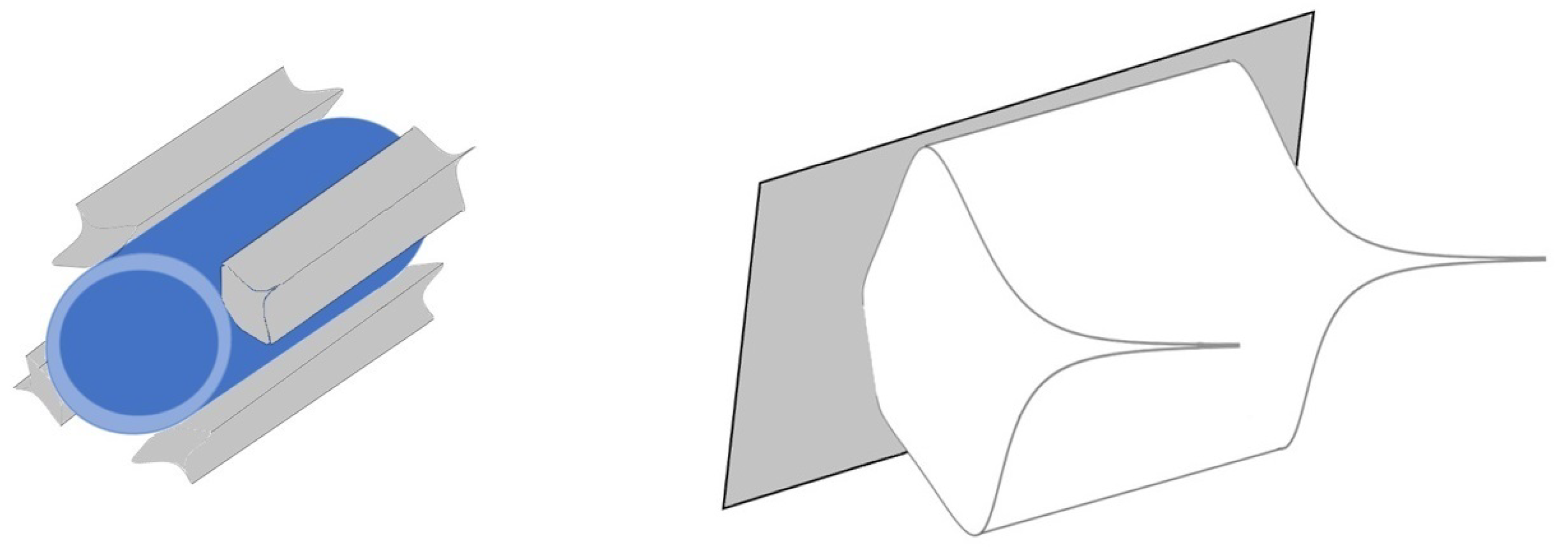
2. Description of the Physical Model

In this section, we mainly follow Bochicchio et al. [4] and one of our previous works [6]. A longitudinal fin of arbitrary profile is attached to a source base at a fixed temperature $T_b$. The fin length (alongside the base) is L, whereas the fin thickness at a distance x from the base is $2f_0\left(x\right)\ge 0$. We consider a symmetric fin: the profile is described by the curves $f_0\left(x\right)$ and $-f_0\left(x\right)$, where x is the coordinate in the direction perpendicular to the fin base. The half-thickness at the base is $f_b=f_0(x=0)$. The fin tip, at $x=\ell$, has half-thickness equal to $f_t=f_0(\ell )$ (see also Figure 1). Following Kraus et al. [1], Nguyen and Aziz [3] and Bochicchio et al. [4], we assume that the Fourier law of conduction holds inside the fin and that the temperature varies, due to the symmetries, only along the x direction.

Given $\rho$ the density of the homogeneous material, h the convective heat transfer coefficient, $\kappa$ the thermal conductivity, c the specific heat, and $\sigma$ the Stefan-Boltzmann constant, the evolution of temperature $T(x,t)$ is governed by the following equation [4]:

$$\rho c{f}_0\left(x\right)\frac{\partial T}{\partial t}=\kappa \frac{\partial }{\partial x}\left(f_0\left(x\right)\frac{\partial T}{\partial x}\right)-2h(T-T_0)-2\sigma ϵ(T^4-T_0^4)$$

(1)

where $ϵ$ is the emissivity of the fin and $T_0$ is the temperature of the fluid adjacent to the fin. In the rest of this paper we are interested in the steady-state distribution of the temperature along the fin, so the equation we are looking for is

$$\kappa \frac{\partial }{\partial x}\left(f_0\left(x\right)\frac{\partial T}{\partial x}\right)-2h(T-T_0)-2\sigma ϵ(T^4-T_0^4)=0.$$

(2)

The boundary conditions are in general determined by the Biot and radiation-convection numbers of the base and of the tip of the fin. In general we must have:

$$f_0\left(x\right){\left.\frac{dT}{dx}\right|}_{x=0}-{\left.{\eta }_0(T-T_b)\right|}_{x=0}-{\xi }_0{\left.(T^4-T_b^4)\right|}_{x=0}=0.$$

(3)

and

$$f_0\left(x\right){\left.\frac{dT}{dx}\right|}_{x=\ell }+{\left.{\eta }_1(T-T_0)\right|}_{x=\ell }+{\xi }_1{\left.(T^4-T_0^4)\right|}_{x=\ell }=0.$$

(4)

where ${\eta }_i$ and ${\xi }_i$, $i=0,1$, are proportional to the corresponding Biot and radiation-conduction numbers.

Let us introduce dimensionless variables. We set $z=x/\ell$, $\theta =T/T_b$, $\alpha =2h{\ell }^2/\left(f_b\kappa \right)$, $\beta =2\sigma ϵ{\ell }^2{T}_b^3/\left(f_b\kappa \right)$ and $f\left(z\right)=f_0(z\ell )/f_b$. Equation (2) becomes

$$\frac{\partial }{\partial z}\left(f\left(z\right)\frac{\partial \theta }{\partial z}\right)-\alpha (\theta -{\theta }_0)-\beta ({\theta }^4-{\theta }_0^4)=0$$

(5)

with boundary conditions

$$\begin{array}{cc}\hfill & {\left.f\left(z\right)\frac{d\theta }{dz}\right|}_{z=0}-{\left.B{i}_0(\theta -1)\right|}_{z=0}-{\left.N_0({\theta }^4-1)\right|}_{z=0}=0,\hfill \\ \hfill & {\left.f\left(z\right)\frac{d\theta }{dz}\right|}_{z=1}+{\left.B{i}_1(\theta -{\theta }_0)\right|}_{z=1}+{\left.N_1({\theta }^4-{\theta }_0^4)\right|}_{z=1}=0,\hfill \end{array}$$

(6)

where the radiation–conduction numbers $N_j={\xi }_j\ell /f_b$, $j=0,1$ and the Biot numbers $B{i}_j={\eta }_j\ell /f_b$, $j=0,1$, have been introduced.

Equation (5) is nonlinear in $\theta$ and, in general, cannot be solved explicitly in terms of known functions. Some explicit solutions and a methodology to find exact solutions of Equation (5) has been described by Bochicchio et al. [4]. In the next section we introduce the entropic efficiency of the fin.

3. The Entropic Efficiency

The definition of the entropic efficiency ${\eta }_s$, given by the authors of this paper in [6], is the ratio between the entropy produced by the fin during the evolution of the system from the initial temperature $T_0$ to the steady state T with respect to the entropy produced by the fin by evolving the system from the same initial distribution $T_0$ to the reference temperature $T_b$. In formulae, we have:

$${\eta }_s\doteq \frac{{\int }_0^1\left({\dot{s}}_{0,\sigma }({\theta }^3-{\theta }_0^3)+{\dot{s}}_{0,h}ln\left(\frac{\theta }{{\theta }_0}\right)\right)dz}{\left({\dot{s}}_{0,\sigma }(1-{\theta }_0^3)+{\dot{s}}_{0,h}ln\left(\frac{1}{{\theta }_0}\right)\right)}.$$

(7)

In the previous formula ${\dot{s}}_{0,\sigma }$ and ${\dot{s}}_{0,h}$ are two reference entropies: they are the entropies produced by the fin by evolving the system from $T_{in}$ to $exp\left(1\right)T_{in}$ and from $T=0$ to $T=T_b$. The ratio between the reference entropies ${\dot{s}}_{0,\sigma }$ and ${\dot{s}}_{0,h}$ is related to the ratio of the dimensionless convective and radiative coefficients $\alpha$ and $\beta$ through the formula

$$\frac{{\dot{s}}_{0,\sigma }}{{\dot{s}}_{0,h}}=\frac{16}{3}\frac{I\left(ϵ\right)}{ϵ}\frac{\beta }{\alpha }.$$

(8)

In the previous formula $I_{ϵ}$ describes the dependence of the radiation entropy by emissivity, and, for any fixed $ϵ\in [0,1]$, it is given by the following integral (see e.g., del Rio and de la Selva [14] or Schwabl [15]):

$$I\left(ϵ\right)={\int }_0^{\infty }{x}^2\left[\left(1+\frac{ϵ}{e^x-1}\right)ln\left(1+\frac{ϵ}{e^x-1}\right)-\left(\frac{ϵ}{e^x-1}\right)ln\left(\frac{ϵ}{e^x-1}\right)\right]dx.$$

(9)

Hence, Equation (7) can be written also in this form:

$${\eta }_s=\frac{{\int }_0^1\left(\frac{16}{3}\frac{I\left(ϵ\right)}{ϵ}\beta ({\theta }^3-{\theta }_0^3)+\alpha ln\left(\frac{\theta }{{\theta }_0}\right)\right)dz}{\left(\frac{16}{3}\frac{I\left(ϵ\right)}{ϵ}\beta (1-{\theta }_0^3)+\alpha ln\left(\frac{1}{{\theta }_0}\right)\right)}.$$

(10)

In the next section we start the analysis of formulae (10) and (5) by looking at a purely convective fin: in this case $\beta =0$ and we will try to investigate how the changes in the fin profile $f\left(z\right)$ have effect on the values of the efficiency ${\eta }_s$ (10).

4. The Case of Non-Radiating Fins

We start our analysis by looking at the case when the radiative contribution to the dissipation of heat can be neglected. In this case the efficiency ${\eta }_s$ is given by

$${\eta }_s=1-\frac{1}{ln\left({\theta }_0\right)}{\int }_0^{1}ln\left(\theta \right)dz$$

(11)

A systematic investigation about the optimal profile $f\left(z\right)$ of the fin, together with the optimal choice of the material characteristics (convective properties related to the convective coefficient $\alpha$ and to the Biot number $Bi$) seems to be difficult to perform directly through variational techniques. In Equation (11) it appears the temperature directly that however is coupled to the profile $f\left(z\right)$ in Equation (5). The optimal choice may also depend on the choice of the boundary conditions. For this reason we capsize the point of view. We look at different temperature profiles across the fin with different parametric families of functions. Among these we select the family possessing the highest efficiency. It is not difficult to understand, from formula (11), the characteristics of the temperature distribution possessing high efficiency. Indeed, $\theta$ assumes values in the range $[{\theta }_0,1]$ and, physically, we expect it to be a decreasing function of z. This implies that the value of the area under the graph of $\theta \left(z\right)$ between $z=0$ and $z=1$ must be as large as possible (see also Figure 2).

Once the temperature distribution is fixed, the profile of the fin is calculated by solving Equation (5) for $f\left(z\right)$. Indeed, for any fixed $\theta \left(z\right)$, Equation (5) is a differential equation for the function $f\left(z\right)$ that can be explicitly solved. For the case of a non-radiating fin we obtain

$$f\left(z\right)=\frac{c+\alpha {\int }_0^z(\theta \left(x\right)-{\theta }_0)dx}{\frac{d\theta }{dz}},$$

(12)

where the value of c is a constant of integration and must be fixed by requiring, consistently with the definition of $f\left(z\right)$, that $f\left(0\right)=1$. The choice of the classes of functions for $\theta \left(z\right)$ must satisfy the given boundary conditions. We take the base of the fin to be at $T=T_b$, i.e., $\theta \left(0\right)=1$. The convection on the fin tip is described by the corresponding Biot number: at the fin tip then we have

$${\left.f\left(z\right)\frac{d\theta }{dz}\right|}_{z=1}+{\left.Bi(\theta -{\theta }_0)\right|}_{z=1}=0.$$

(13)

The limit case $Bi=0$ corresponds to an insulated tip, whereas the limit $Bi\to \infty$ corresponds to a tip at $T=T_0$. Here we will discuss the two limiting cases: the first one is that of a tip at $T=T_0$, i.e., we take:

$$\theta \left(1\right)={\theta }_0$$

(14)

The second one is the case of a fin with an insulated tip, i.e.

$${\left.\frac{d\theta }{dz}\right|}_{z=1}=0.$$

(15)

4.1. Tip at $T=T_0$

Given Equation (5), from an analytical point of view the simplest situation is to consider a rectangular fin, corresponding, in dimensionless variables, to $f\left(z\right)=1$. In this case it is possible to solve Equation (5) (when $\beta =0$) exactly. The solution, corresponding to the given boundary conditions, is

$$\theta \left(z\right)={\theta }_0+(1-{\theta }_0)\frac{sinh\left(m\right(1-z\left)\right)}{sinh\left(m\right)}.$$

(16)

where $m=\sqrt{\alpha }$. If the fin profile changes, the steady-state temperature distribution will not be (16), but will change accordingly to Equation (5). Vice versa, if we change the temperature profile, the fin profile will change according to Equation (5). As explained in the lines above, we would like to expand the area under the graph of $\theta \left(z\right)$, stretching up the temperature distribution. We start from formula (16). Since $z\in [0,1]$, we substitute to z in formula (16) a non-negative function $g\left(z\right)$ such that $g\left(z\right)<z$ for $z\in [0,1]$. For the sake of simplicity, let us take $g\left(z\right)=z^k$, where k is a given parameter. The new temperature distribution that we consider is then the following:

$$\theta \left(z\right)={\theta }_0+(1-{\theta }_0)\frac{sinh\left(m(1-z^k)\right)}{sinh\left(m\right)}.$$

(17)

Notice that the functions (17) satisfy the same boundary conditions for any k. The effect of inserting the power $z^k$ can be better understood by looking at Figure 3.

Additionally, if the class of functions (17) is expected to give more efficient fins, one should keep in mind that Equation (12) for the profile of the fin must give physically reasonable functions, i.e., it should have no singularities in $z\in [0,1]$ and should be non-negative in this interval. The dependence on powers of the type $z^k$ can give difficulties in this regard: indeed, if $k>1$, the derivative in the denominator of Equation (12) vanishes and singularities appear in the function $f\left(z\right)$. Since ${\eta }_s$ is an increasing function of k, this means that the value $k=1$ (i.e., $\theta$ given by Equation (16)) gives the maximum physically admissible efficiency. Then, with the position (17) there is no possibility to enhance the efficiency of the basic, rectangular, fin.

The problem is the value of the derivative of the function (17) at $z=0$: as can be seen also from Figure 3, the function is flattened around $z=0$ for $k>1$ and its derivative vanishes at $z=0$. Locally around $z=0$ we would need a temperature distribution with a finite negative derivative, flattening in the middle, such as a logistic curve turned upside down. A possibility is to add to the distribution (17) a function vanishing both in $z=0$ and $z=1$ (so that the effect on the boundary conditions is null) and with a small negative value. The simplest choice is the polynomial $-z(1-z^{\frac{1}{n}})$. We also insert a new parameter, say w, in order to have control of this term. Therefore, we consider the new class of distributions temperature as

$$\theta \left(z\right)=-wz(1-z^{\frac{1}{n}})+{\theta }_0+(1-{\theta }_0)\frac{sinh\left(m(1-z^k)\right)}{sinh\left(m\right)}.$$

(18)

To give an idea of the effect of introducing the term proportional to w, we plot in Figure 4 the temperature distribution for three different values of k and for $w=0$ and $w=0.1$. To the red distribution, corresponding to $w=0$, there correspond higher values of the efficiency (11), but, as said above, the flatness of the curves at $z=0$ gives a singularity to the profile in $z=0$: this conclusion can be compared with similar singularities results described in [10]. The effect of having $w\ne 0$ is to increase the absolute value of the derivative at $z=0$, avoiding the singularity problem.

We notice that, for any fixed value of ${\theta }_0$ and m, the efficiency (11) is increasing by increasing k and n and decreasing by increasing w (see for example Figure 5).

Therefore, it should be advantageous to take the highest possible value of k and n and small values of w. However, again we are constrained by physical considerations on the profile of the fin in the possible choices of these three parameters. Indeed, for any fixed couple $(n,k)$ we see that it exists a threshold value $w^{*}$ such that $f\left(1\right)<0$ for $w<w^{*}$ and $f\left(1\right)>0$ for $w>w^{*}$. Furthermore, for large values of k, the values of $f\left(z\right)$ in the range $z\in (0,1)$ could have quite high peaks. It is clear that the value of $f\left(z\right)$ at some point between $z=0$ and $z=1$ cannot be arbitrarily high. For example, if the fin is a component of an array the space available depends on the spacing. Additionally, usually there are compelling space limitations in physical and electronic systems. In general, we may say that there should be some threshold value for the maxima of $f\left(z\right)$, $z\in [0,1]$. The value of this threshold depends on the type of application and physical conditions in which the fin must operate. In the following, we will make a choice for the threshold to show how our approach works. It should be kept in mind however that this value has been chosen for an illustrative purpose and must be adapted to the particular application to maximize the efficiency (11).

Therefore, to be operative, let us choose the value of 4 as the maximum value for the value of $f\left(z\right)$, $z\in [0,1]$. We remember that the half-thickness of the fin at its base is $f_b$, so, in dimensional units, the base thickness is $2f_b$, whereas the total thickness is not greater than $8f_b$ if the maximum value for the value of $f\left(z\right)$ is 4.

In the following we start the analysis by fixing $k=2$ and trying to vary the parameters $(n,w)$. Then we will look at further values of k. To fix the ideas, the values of the parameters ${\theta }_0$ and m are fixed to be ${\theta }_0=1/2$ and $m=1$.

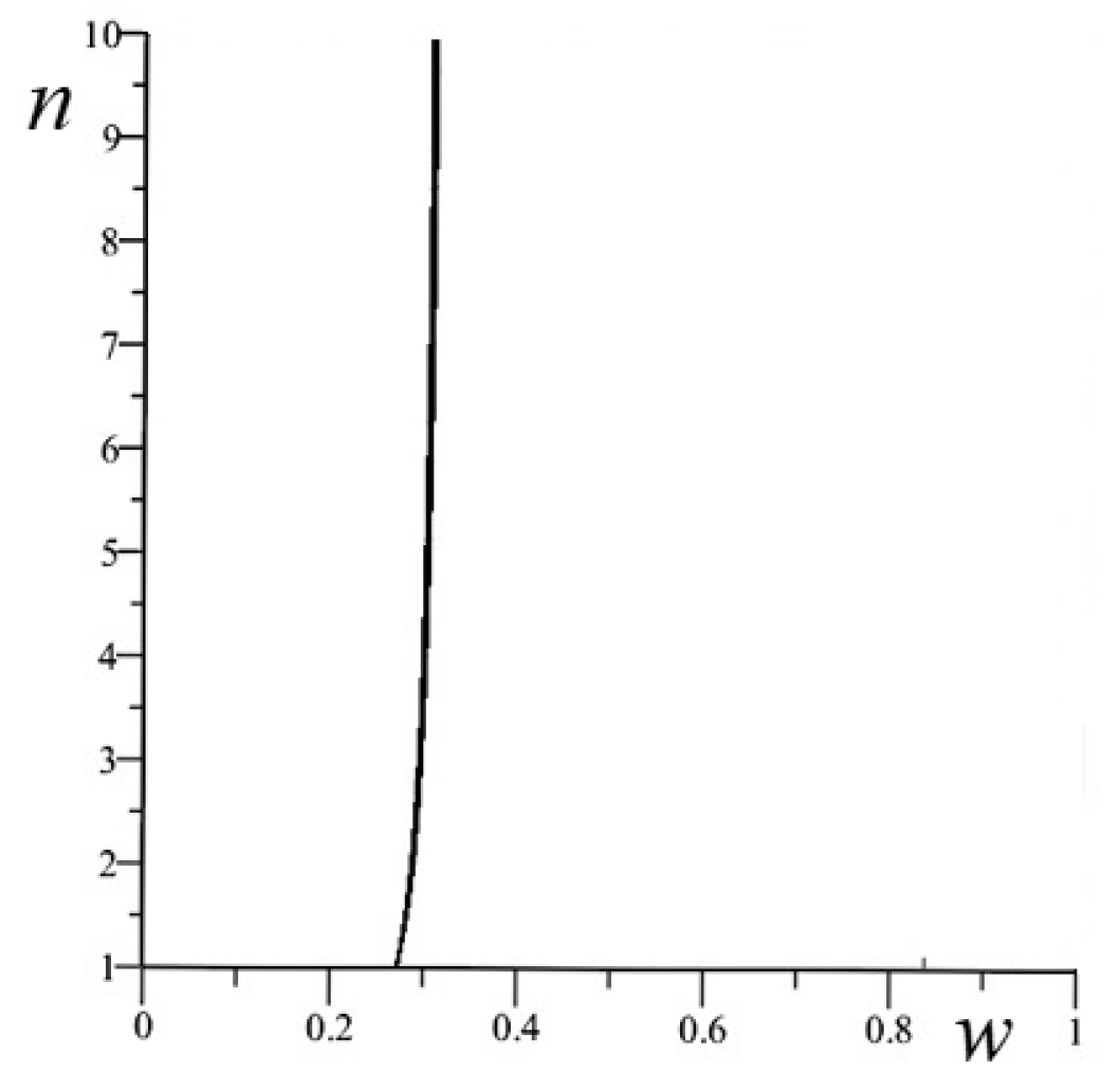
• $k=2$. For small of w and large n the value of the efficiency (11) is ∼ 0.68. Numerically we see that $f\left(1\right)>0$ only if $w>w_2^{*}$, where $w_2^{*}$ is a certain value of w that depends also on n. A plot of $w_2^{*}$ as a function of n is reported in Figure 6. It is possible to show that for n large and for the given values of ${\theta }_0$ and m, $w_2^{*}$ is asymptotic to 0.3174…

Figure 6. The values of the threshold $w_2^{*}$ for $k=2$ as a function of n: only for $w>w_2^{*}$$f\left(1\right)>0$.

Figure 6. The values of the threshold $w_2^{*}$ for $k=2$ as a function of n: only for $w>w_2^{*}$$f\left(1\right)>0$.

If we choose w just above the threshold $w_2^{*}$. i.e., $w=0.318$, the corresponding profile of the fin $f\left(z\right)$ for $n=10$ is given in Figure 7. The corresponding efficiency can be calculated to be ∼0.668. For comparison, with $k=1$ and $w=0$ we have an efficiency ∼0.52.

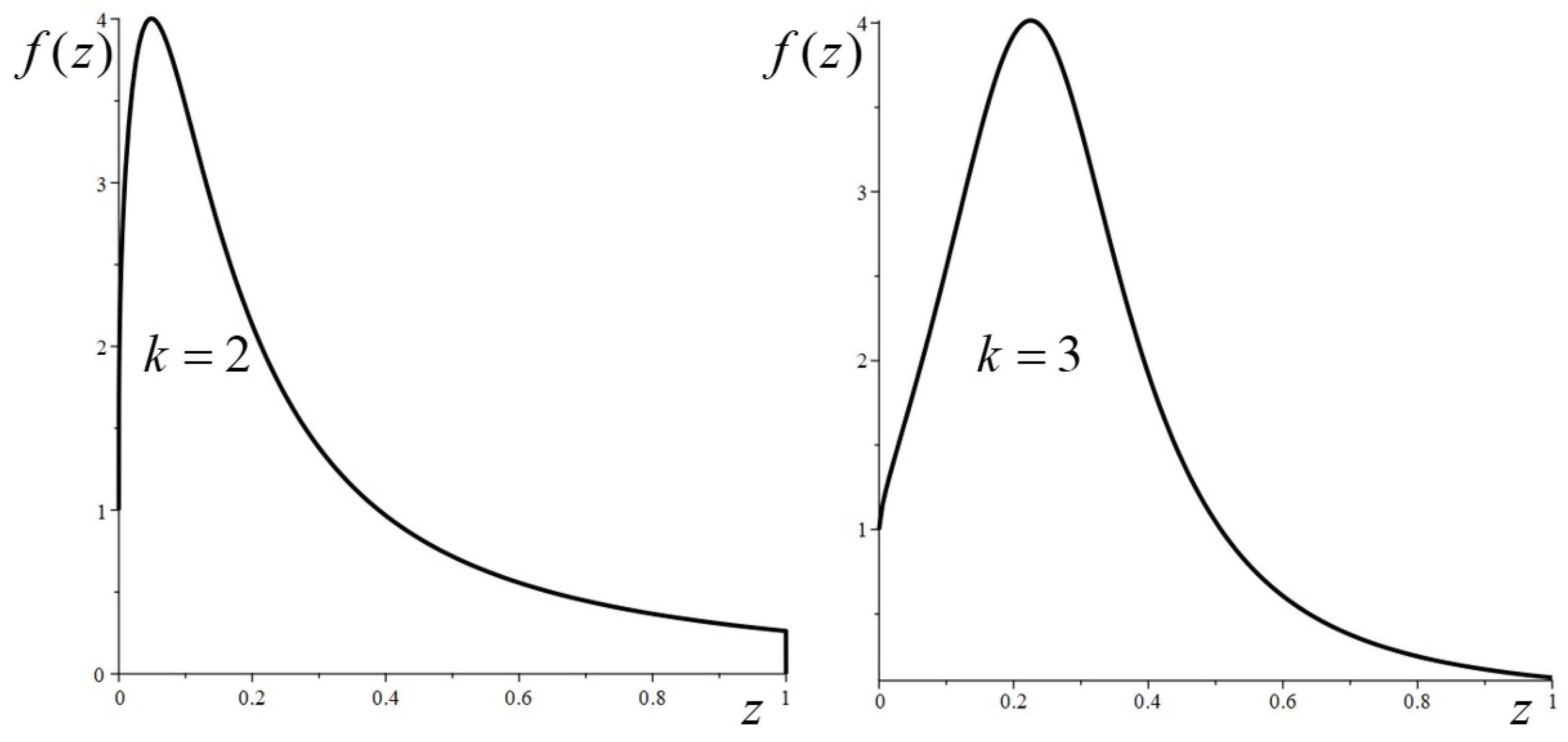
• $k=3$. Again, we have a threshold $w_3^{*}$ such that $f\left(1\right)>0$ only if $w>w_3^{*}$. For n large $w_3^{*}$ is asymptotic to 0.361... We take $w=0.362$. The asymptotic maximum value of the efficiency, if $k=3$, is given by $0.761...$. This is the maximum value for the given parameters m, ${\theta }_0$, k and w, obtained for large n. However, for large values of n, the maximum of $f\left(z\right)$ becomes greater than four. There is another threshold value, this time for n, given by $n\sim 7.61$, such that the maximum of $f\left(z\right)$ is not greater than four. Therefore, we take $n=7.6$. The corresponding value of the efficiency is ${\eta }_s\sim 0.743$. The fin profile is reported in (Figure 8).
• $k=4$. We have a threshold $w_4^{*}$ such that $f\left(1\right)>0$ only if $w>w_4^{*}$. For n large $w_4^{*}$ is asymptotic to 0.389... We take $w=0.39$. The asymptotic maximum value of the efficiency is given by $0.809...$. However, for large values of n, the maximum of $f\left(z\right)$ becomes greater than four. The threshold value for n (such that the maximum of $f\left(z\right)$ is not greater than 4) is now given by $n\sim 4.7$. Therefore, we take $n=4.7$. The value of the efficiency is ${\eta }_s\sim 0.793$.
• $k=5$. We have a threshold $w_5^{*}$ such that $f\left(1\right)>0$ only if $w>w_5^{*}$. For n large $w_5^{*}$ is asymptotic to 0.407... We take $w=0.41$. The asymptotic maximum value of the efficiency in this case is given by $0.841...$. There is a threshold value for n, given by $n\sim 3.18$, such that the maximum of $f\left(z\right)$ is not greater than four. Therefore, we take $n=3.17$. The value of the efficiency is ${\eta }_s\sim 0.797$. Actually, for small values of n, it would be possible to take some smaller values of w with respect to $w_5^{*}$ (since $w_5^{*}$ actually depends on n). But the difference in the efficiencies is not really large. The fin profile is reported in Figure 9.
• $k=6$. We have a threshold $w_6^{*}$ such that $f\left(1\right)>0$ only if $w>w_6^{*}$. For n large $w_6^{*}$ is asymptotic to 0.420... We take $w=0.421$. The asymptotic maximum value of the efficiency in this case is given by $0.863...$. The threshold value for n is now given by $n\sim 2.05$. Therefore, we take $n=2.04$. The corresponding value of the efficiency is ${\eta }_s\sim 0.799$.

We see that for $k=6$ the efficiency is very close to that of the case $k=5$. Indeed, by increasing k, we need to take smaller values for the threshold n to avoid greater values for the maximum of $f\left(z\right)$. This is clearly a physical constraint but, as said, it should be kept in mind that it depends on the suitable application and conditions in which the fin operates and as such can be modified.

4.2. The Insulated Tip

It is well known that the efficiency of a fin is a decreasing function of the Biot number $Bi$. From our point of view this is a consequence of the fact that, in general, for lower Biot numbers the tip temperature will be higher, giving a greater area under the curve $\theta \left(z\right)$, $z\in [0,1]$. In this subsection we apply the same scheme of the previous subsection: we start from the temperature distribution corresponding to a rectangular fin and then we try to modify it be keeping the same boundary conditions but increasing the area under the curve $\theta \left(z\right)$. When $f\left(z\right)=1$ and with the given boundary conditions, the temperature distribution is

$$\theta \left(z\right)={\theta }_0+(1-{\theta }_0)\frac{cosh\left(m\right(1-z\left)\right)}{cosh\left(m\right)}.$$

(19)

Again, we consider as ground distribution the function (19) by substituting $z\to z^k$. Then we add a function vanishing at $z=0$ and with the derivative at $z=1$ equal to zero. Additionally, we require that the derivative at $z=0$ to be negative. By requiring this function to be of the form $\sim z(1+az+b{z}^{1/n})$ we obtain

$$\theta \left(z\right)=-wz(1-z^{\frac{1}{n}}-\frac{1-z}{n})+{\theta }_0+(1-{\theta }_0)\frac{cosh\left(m(1-z^k)\right)}{cosh\left(m\right)}.$$

(20)

We notice that now, differently with respect to the previous case, w and n are not arbitrary but there should be a relation between them. Indeed, to be consistent and avoid a singularity in $f\left(z\right)$ at $z=1$, we must re-write Equation (12) in this form:

$$f\left(z\right)=\frac{\alpha {\int }_1^z(\theta \left(x\right)-{\theta }_0)dx}{\frac{d\theta }{dz}}.$$

(21)

Now, for fixed values of the parameters m, k and ${\theta }_0$, the constraint $f\left(0\right)=1$ can be seen as an equation determining the value of n as a function of w or vice-versa. Indeed, it can be shown that there is a polynomial of second degree in n linking w to n. It is explicitly given by:

$$12n^2(w-m^{2}a)-n((6-m^2)w+6m^{2}a)-w(6+m^2)=0,$$

(22)

where

$$a={\int }_0^1(1-{\theta }_0)\frac{cosh\left(m(1-z^k)\right)}{cosh\left(m\right)}.$$

Then, the value of w must be fixed to be

$$w=\frac{6a{m}^{2}n(2n+1)}{(n-1)(m^2+12n+6)}.$$

(23)

With this choice of w we have only another two free parameters (i.e., k and n) to control to maximize the efficiency. Again, as in the previous subsection, the parameter n, for any fixed k, must be fixed by requiring that the maximum of $f\left(z\right)$ should not be greater than a threshold value, again fixed to be 4 here. So let us start to describe what happens for successive values of k. For all this subsection the values of the parameters ${\theta }_0$ and m are fixed to be ${\theta }_0=1/2$ and $m=1$. For comparison with what presented below, the value of the efficiency corresponding to the temperature distribution (19) with ${\theta }_0=1/2$ and $m=1$ is ${\eta }_s\sim 0.814$.

• $k=2$. All the parameters are fixed apart n. As a function of n the efficiency is an increasing function, with an asymptotic value equal to 0.870.... However, for n greater than 7.26 the function $f\left(z\right)$ has a maximum greater than 4. Therefore, we take $n=7.25$. The corresponding value of the efficiency is 0.863.
• $k=3$. As a function of n now the efficiency is asymptotic to ∼0.9. However, the threshold on n giving a maximum of $f\left(z\right)$ greater than four is very small: it is given by $n=1.52$. We take $n=1.51$. The corresponding value of the efficiency is ∼ 0.874.
• $k=4$. The efficiency is asymptotic to ∼0.92. For this value of k the threshold value of n is smaller than 1: the corresponding value of the efficiency is smaller than the previous, giving an optimal value of k equal to 3.

The plots of the fin profile corresponding to $k=2$ and $k=3$ analyzed above are given in Figure 10.

4.3. Comparison with the Classical Definition of the Efficiency for Non-Radiating Fins

The classical definition of efficiency relies on the first principle of thermodynamics, i.e., the efficiency is measured in terms of the heat transferred by the fin to the external environment. More precisely the classical efficiency $\eta$ is given by the ratio of the actual heat transfer to the ideal heat transfer for a fin of infinite thermal conductivity (i.e., at $T=T_b$ or $\theta =1$). For non-radiating fins it is possible to show that, in terms of dimensionless variables, such efficiency is explicitly given by

$$\eta =\frac{{\left.f\left(z\right)\frac{d\theta }{dz}\right|}_{z=1}-{\left.f\left(z\right)\frac{d\theta }{dz}\right|}_{z=0}}{\alpha (1-{\theta }_0)}$$

(24)

We notice that the previous formula can be usefully rewritten in another form. Indeed, we have

$$\eta =\frac{{\left.f\left(z\right)\frac{d\theta }{dz}\right|}_{z=1}-{\left.f\left(z\right)\frac{d\theta }{dz}\right|}_{z=0}}{\alpha (1-{\theta }_0)}=\frac{{\int }_0^1\frac{d}{dz}\left(f\left(z\right)\frac{d\theta }{dz}\right)dz}{\alpha (1-{\theta }_0)}$$

(25)

and, from the differential Equation (5)

$$\eta ={\int }_0^1\left(\frac{\theta \left(z\right)-{\theta }_0}{1-{\theta }_0}\right)dz.$$

(26)

The comparison of this definition with the entropic one (11) that can be also rewritten as

$${\eta }_s={\int }_0^1\left(1-\frac{ln\left(\theta \right(z\left)\right)}{ln\left({\theta }_0\right)}\right)dz$$

(27)

has been given by Bochicchio et al. in [4]. Here we want just to notice that both the integrands are increasing functions of $\theta \left(z\right)$, but the integrand of ${\eta }_s$ is concave with respect to $\theta \left(z\right)$: this means that ${\eta }_s\ge \eta$. As it has been shown in [4], this property is not fulfilled if the effects of radiation are taken into account. Additionally, the same line of reasoning adopted to maximize the nonlinear efficiency can be adopted for the classical definition: since the integrand increases with the temperature, this implies that, in order to maximize the efficiency, we must take a value of the area under the graph of $\theta \left(z\right)$ between $z=0$ and $z=1$ as large as possible. The same distributions of temperature considered in the previous section are expected to represent an optimal choice for the maximization of the efficiency.

In

Table 1. The steady states considered in Section 2 and the corresponding efficiencies.

$\mathit{\theta }\left(\mathit{z}\right)$	$\mathit{\eta }$	${\mathit{\eta }}_{\mathit{s}}$
$\frac{1}{2}+\frac{1}{2}\frac{sinh\left(\right(1-z\left)\right)}{sinh\left(1\right)}.$	0.462	0.520
$-0.318z(1-z^{\frac{1}{10}})+\frac{1}{2}+\frac{1}{2}\frac{sinh\left((1-z^2)\right)}{sinh\left(1\right)}.$	0.619	0.668
$-0.362z(1-z^{\frac{1}{7.6}})+\frac{1}{2}+\frac{1}{2}\frac{sinh\left((1-z^3)\right)}{sinh\left(1\right)}.$	0.701	0.743
$-0.39z(1-z^{\frac{1}{4.7}})+\frac{1}{2}+\frac{1}{2}\frac{sinh\left((1-z^4)\right)}{sinh\left(1\right)}.$	0.740	0.779
$-0.41z(1-z^{\frac{1}{3.17}})+\frac{1}{2}+\frac{1}{2}\frac{sinh\left((1-z^5)\right)}{sinh\left(1\right)}.$	0.758	0.797
$-0.421z(1-z^{\frac{1}{2.04}})+\frac{1}{2}+\frac{1}{2}\frac{sinh\left((1-z^6)\right)}{sinh\left(1\right)}.$	0.758	0.799
$\frac{1}{2}+\frac{1}{2}\frac{cosh\left(\right(1-z\left)\right)}{cosh\left(1\right)}.$	0.761	0.814
$-0.477z(1-z^{\frac{1}{7.25}}-\frac{1-z}{7.25})+\frac{1}{2}+\frac{1}{2}\frac{cosh\left((1-z^2)\right)}{cosh\left(1\right)}.$	0.823	0.863
$1.238z(1-z^{\frac{1}{1.51}}-\frac{1-z}{1.51})+\frac{1}{2}+\frac{1}{2}\frac{cosh\left((1-z^3)\right)}{cosh\left(1\right)}.$	0.836	0.875

, we report the values of the classical and entropic efficiencies (26) and (27): on the top of the table, on the first six rows, there are the distributions of temperature corresponding to the boundary conditions $\theta \left(0\right)=1$ and $\theta \left(1\right)=0$. The boundary conditions satisfied by the distributions of temperature in the last three rows are $\theta \left(0\right)=1$ and ${\left.\frac{d\theta }{dz}\right|}_{z=1}=0$.

5. Profile Optimization of the Convecting–Radiating Fin

For convecting–radiating fins, the entropic efficiency is given, in terms of dimensionless variables, by Equation (10):

$${\eta }_s=\frac{{\int }_0^1\left(\frac{16}{3}\frac{I\left(ϵ\right)}{ϵ}\beta ({\theta }^3-{\theta }_0^3)+\alpha ln\left(\frac{\theta }{{\theta }_0}\right)\right)dz}{\left(\frac{16}{3}\frac{I\left(ϵ\right)}{ϵ}\beta (1-{\theta }_0^3)+\alpha ln\left(\frac{1}{{\theta }_0}\right)\right)}.$$

(28)

This is again an increasing function of $\theta \left(z\right)$ and we can adopt the same methodology used in the previous section to optimize the fin profile: we look at some suitable distribution of temperature, with large area under its graph between $z=0$ and $z=1$, and assume that this distribution satisfy the steady state corresponding to Equation (5) with some prescribed boundary conditions. Then, we look at Equation (5) as the equation determining $f\left(z\right)$ and look for the profile, compatible with physical requirements, that maximizes the efficiency (28).

From Equation (28) we see that the value of the efficiency depends only on the ratio $\beta /\alpha$. Let us set $\beta =\alpha y$. In terms of the physical constants of the problem, the value of y is given by

$$\frac{\beta }{\alpha }=y=\frac{\sigma ϵT_b^3}{h},$$

(29)

where we remember that $\sigma$ is the Stefan-Boltzmann constant, $ϵ$ the emissivity of the fin, h the convective heat transfer coefficient and $T_b$ the temperature of the base. If we take values of the emissivity equal to $1/2$ and take $T_b$ to vary in the range $[100,700]K$ and take for h a typical value in the range $[10,1000]\frac{W}{m^{2}K}$, then the possible values of y belong to the range $[0,1]$. The solutions of the nonlinear equation

$$\frac{d}{dz}\left(f\left(z\right)\frac{d\theta }{dz}\right)=\alpha (\theta -{\theta }_0)+\beta ({\theta }^4-{\theta }_0^4)$$

(30)

describing the steady state of the temperature along the fin, cannot be expressed, in general, as expressions involving elementary or special functions. We consider, for simplicity, just one type of boundary conditions: the base of the fin is always at $\theta =1$ and its tip is at $\theta ={\theta }_0$. The case of an isolated tip is more involved since in this case the relation (22) would be quartic in w and of greater degree in n.

Since we do not have an analytic ground distribution temperature, we start from those corresponding to the linear case and then we modify them. In all this section, the values of m (i.e., $\sqrt{\alpha }$), ${\theta }_0$ and $ϵ$ are taken to be equal, respectively, to 1, $1/2$ and $1/2$.

From the same line of reasoning as in Section 4, we consider the family of steady states given by

$$\theta \left(z\right)=-wz(1-z^{\frac{1}{n}})+{\theta }_0+(1-{\theta }_0)\frac{sinh\left(m(1-z^k)\right)}{sinh\left(m\right)}.$$

(31)

The case $w=0$ and $k=1$ corresponds to the distribution temperature solution of Equation (30) for $\beta =0$ and $f\left(z\right)$ equal to a constant. Notice however that the case $w=0$ and $k=1$ can be considered also the solution of Equation (31) for $\beta \ne 0$ and a suitable choice of the fin profile $f\left(z\right)$. Indeed, if we insist that the ground distribution

$$\widehat{\theta }\left(z\right)={\theta }_0+(1-{\theta }_0)\frac{sinh\left(m\right(1-z\left)\right)}{sinh\left(m\right)}$$

(32)

is solution of Equation (30), then, from Equation (30) itself, it follows that $f\left(z\right)$ is given by

$$f\left(z\right)=\frac{{\int }_0^z\left(\alpha (\widehat{\theta }\left(x\right)-{\theta }_0)+\beta ({\widehat{\theta }}^4\left(x\right)-{\theta }_0^4)\right)dx-(1-{\theta }_0)mcoth\left(m\right)}{\frac{d\widehat{\theta }}{dz}}$$

(33)

For $\beta =0$ the previous equation consistently gives $f\left(z\right)=1$, whereas for $\beta \ne 0$$f\left(z\right)$ is decreasing with z. For completeness we report the plot of $f\left(z\right)$ as a function of z and $y=\beta /\alpha$ in Figure 11.

Let us now start the analysis by looking at the variation of the parameters $(n,w)$ in (31) for fixed values of k. We start from $k=2$.

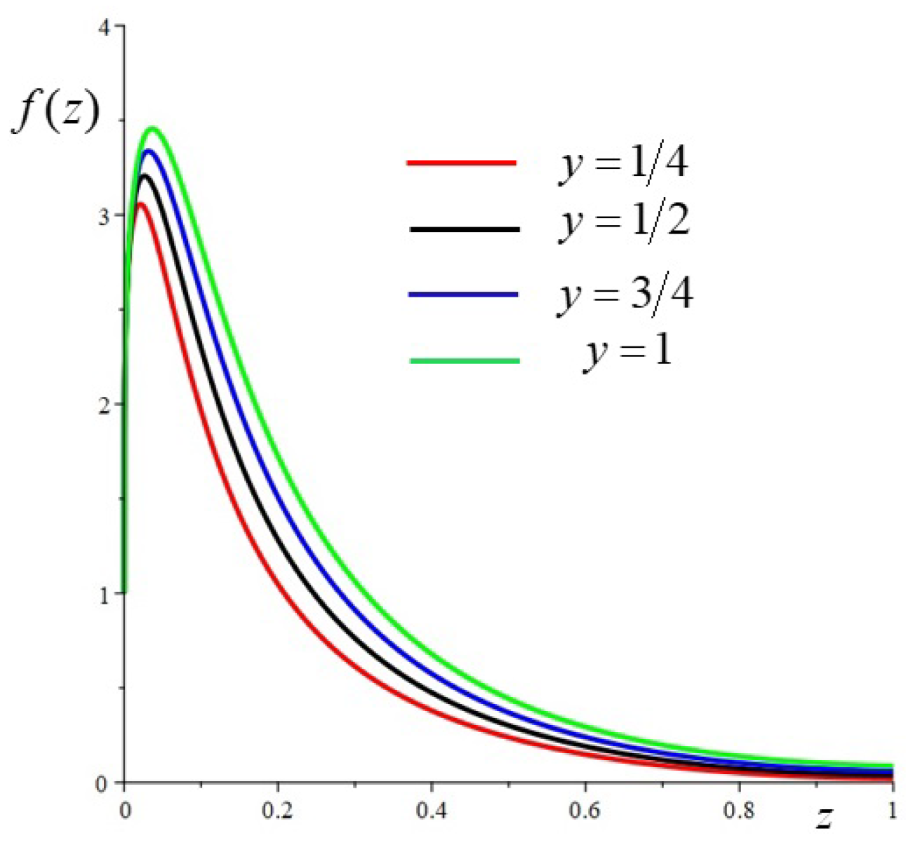
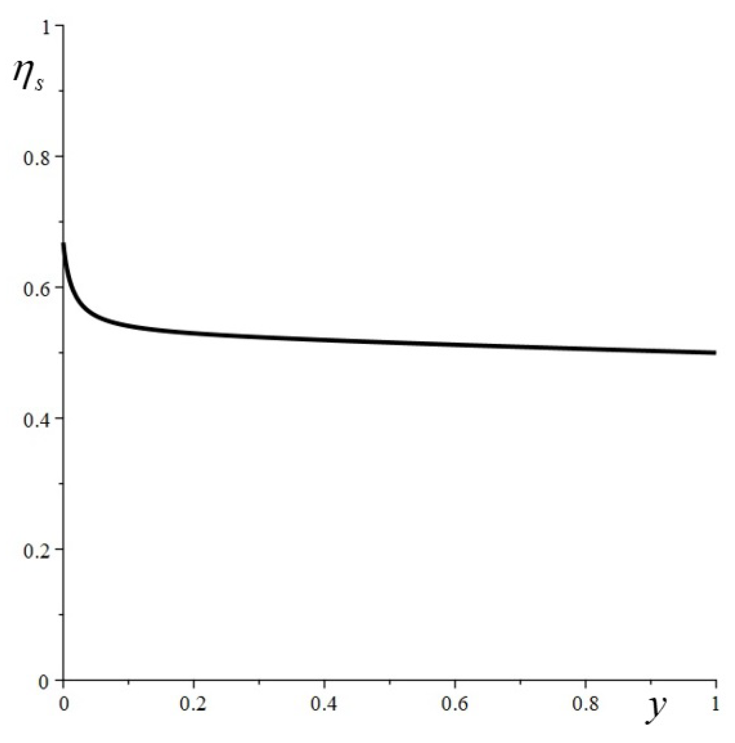
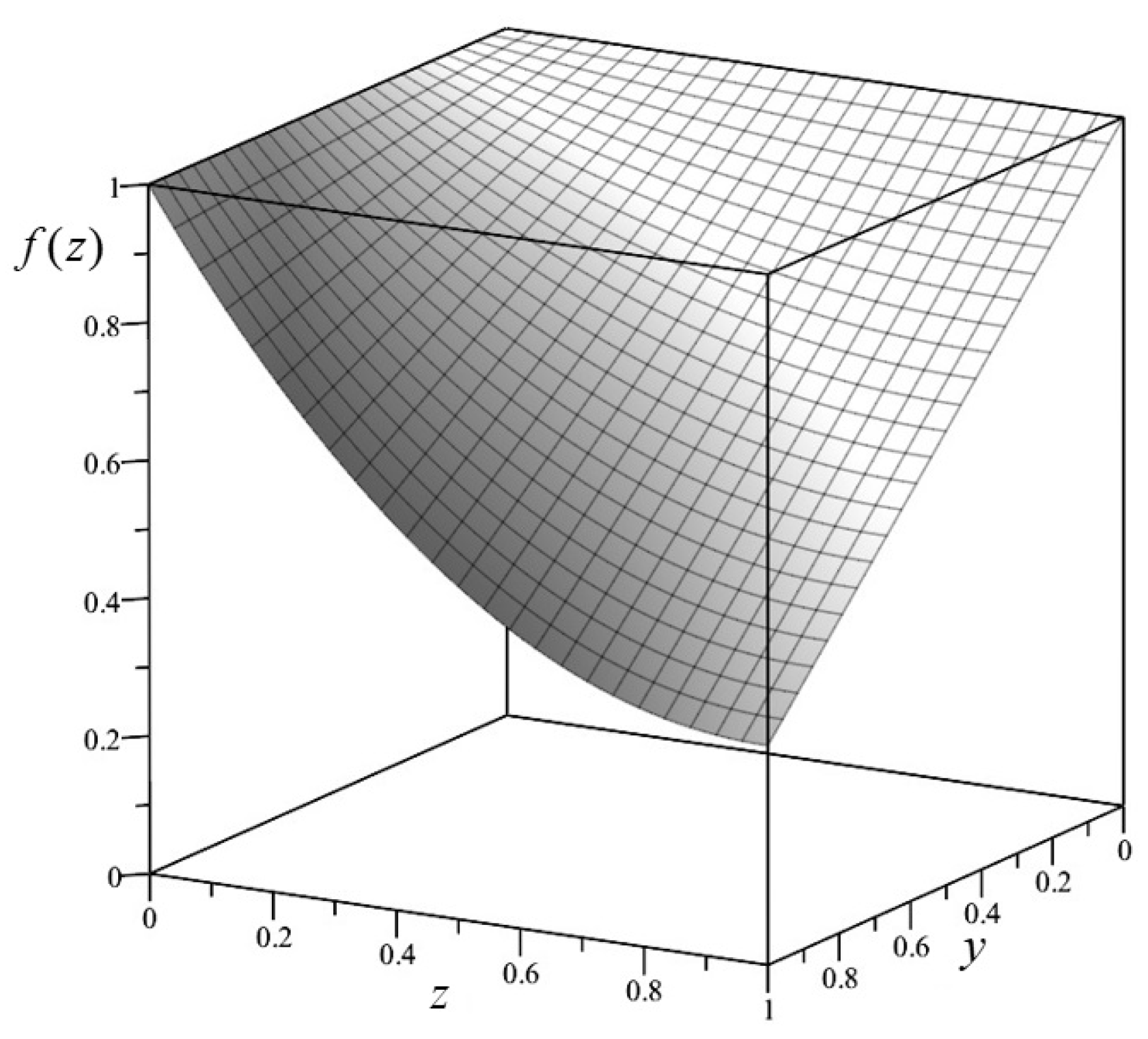
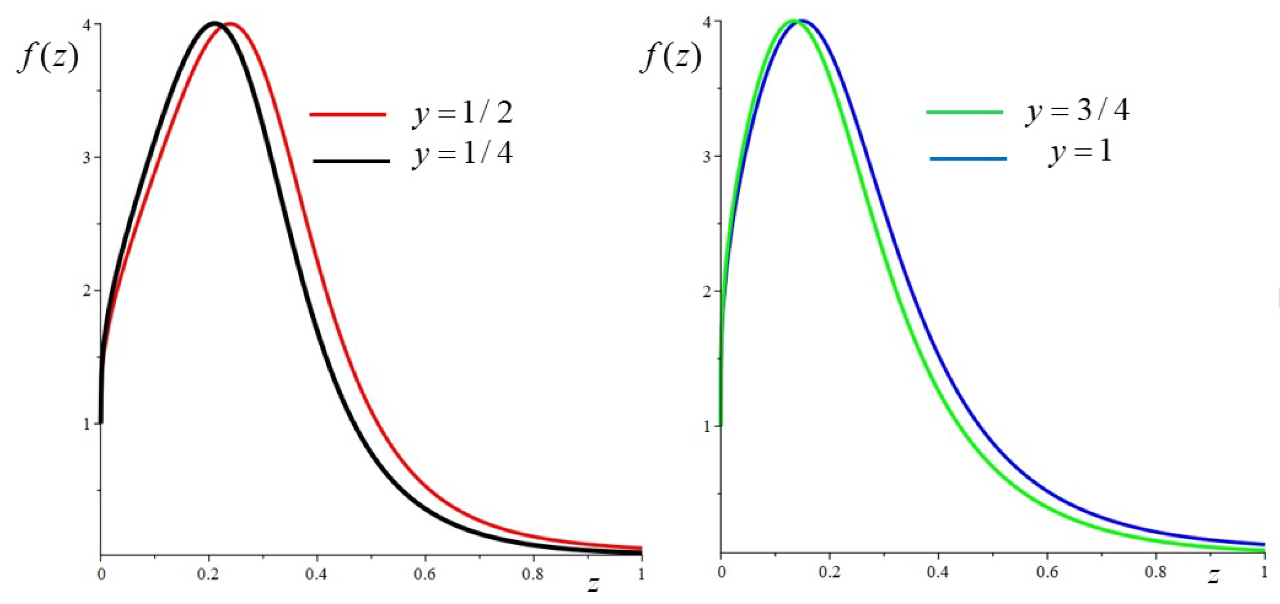
• $k=2$. For fixed values of w and n the value of the efficiency (28) is a function of y. For small w and large n this function is asymptotic, say, to ${\widehat{\eta }}_{s,2}\left(y\right)$. ${\widehat{\eta }}_{s,2}\left(y\right)$ is decreasing with y: it goes from ${\widehat{\eta }}_{s,2}\left(0\right)\sim 0.681$ for $y=0$ to ${\widehat{\eta }}_{s,2}\left(1\right)\sim 0.546$ for $y=1$. Numerically we see that $f\left(1\right)>0$ only if $w>w_2^{*}\left(y\right)$, where $w_2^{*}\left(y\right)$ is a certain value of w that depends on n and y. It is possible to show that for n large and for the given values of ${\theta }_0$ and m, $w_2^{*}\left(y\right)$ is asymptotic to $0.317+0.473y$, so we take $w=0.318+0.473y$. The corresponding profiles for $n=10$ and four values of y are given in Figure 12. The efficiency, with these values of the parameters, is a decreasing function of y from ${\eta }_s\sim 0.668$ for $y=0$ to ${\eta }_s\sim 0.5$ for $y=1$. A plot of ${\eta }_s$ as a function of y is given in Figure 13.
• $k=3$. Again, we see that $f\left(1\right)>0$ only if $w>w_3^{*}\left(y\right)$, where $w_3^{*}\left(y\right)$ is a certain value of w that depends on n and y. It is possible to show that for n large and for the given values of ${\theta }_0$ and m, $w_3^{*}\left(y\right)$ is asymptotic to $0.361+0.577y$, so we take $w=0.362+0.577y$. For any fixed value of $y\in [0,1]$ there is a threshold value of n, ${\widehat{n}}_3\left(y\right)$ such that the maximum of $f\left(z\right)$ is greater than four for $n>{\widehat{n}}_3\left(y\right)$. For $y=\frac{1}{4}$, $\frac{1}{2}$, $\frac{3}{4}$ and 1, the values of ${\widehat{n}}_3\left(y\right)$ are, respectively, given by $7.08$, $6.66$, $6.30$ and $5.98$. By taking values of n just below these thresholds, one obtains the following values of the efficiencies (in order from $y=1/4$ to $y=1$): $0.610$, $0.591$, $0.573$ and $0.553$.
• $k=4$. The threshold value of w, $w_4^{*}\left(y\right)$ is asymptotic, for n large, to $0.389+0.644y$, so we take $w=0.39+0.644y$. For any fixed value of $y\in [0,1]$ there is a threshold value of n, ${\widehat{n}}_4\left(y\right)$ such that the maximum of $f\left(z\right)$ is greater than four for $n>{\widehat{n}}_4\left(y\right)$. For $y=\frac{1}{4}$, $\frac{1}{2}$, $\frac{3}{4}$ and 1, the values of ${\widehat{n}}_4\left(y\right)$ are, respectively, given by $4.38$, $3.99$, $3.61$ and $3.21$. The corresponding efficiencies are given by 0.641, 0.607, 0.571 and 0.528.
• $k=5$. The threshold value of w, $w_5^{*}\left(y\right)$ is now asymptotic, for large n, to $0.407+0.690y$: let us take $w=0.408+0.690y$. The threshold values of n, say ${\widehat{n}}_5\left(y\right)$, such that the maximum of $f\left(z\right)$ is greater than four for $n>{\widehat{n}}_4\left(y\right)$, are the following: ${\widehat{n}}_5\left(y\right)=2.72$ in $y=1/4$, ${\widehat{n}}_5\left(y\right)=2.23$ in $y=1/2$, ${\widehat{n}}_5\left(y\right)=1.70$ in $y=3/4$ and ${\widehat{n}}_5\left(y\right)=0.99$ in $y=1$. The corresponding efficiencies are given by $0.637$, $0.571$, $0.482$ and $0.327$.

Figure 12. The fin profiles for $k=2$, $w=0.318+0.473y$, $n=10$, ${\theta }_0=1/2$ and $m=1$ and four different values of y.

Figure 12. The fin profiles for $k=2$, $w=0.318+0.473y$, $n=10$, ${\theta }_0=1/2$ and $m=1$ and four different values of y.

Figure 13. The efficiency corresponding to the case $k=2$ as a function of y. The other parameters are $w=0.318+0.473y$, $n=10$, ${\theta }_0=1/2$ and $m=1$.

Figure 13. The efficiency corresponding to the case $k=2$ as a function of y. The other parameters are $w=0.318+0.473y$, $n=10$, ${\theta }_0=1/2$ and $m=1$.

We see that, starting from $k=4$ and $y>1/2$, by increasing k we are not increasing the values of the efficiencies: for $y>1/2$ the case $k=3$ is the optimal choice. For $y\le 1/2$ and $y\ne 0$ the optimal choice is $k=4$. The value $y=0$ corresponds to the purely convective case analyzed in the previous section. In Figure 14 we report the profiles corresponding to $k=4$ for $y=1/4$ and $y=1/2$ (left) and the profiles corresponding to $k=3$ for $y=3/4$ and $y=1$ (right): the overall shape of the profiles are quite similar to those of the purely convective case.

6. Analysis of the Results

As can be seen from Figure 9 and Figure 14, the optimal fin profile, according to this study, is increasing starting from the fin base until it reaches a global maximum and then decreases to zero at the tip. The global maximum must be fixed a-priori and is dictated by physical considerations suitable for each specific application of the fin. Physically, the characteristics of the profile to be increasing is because we require that the area under the function $\theta \left(z\right)$, compatibly with the boundary conditions, must be as large as possible for $z\in [0,1]$. This mathematical requirement, if taken as it is, gives a singular function $f\left(z\right)$ in $z=0$ and hence must be balanced by the specification that the profile must be non-singular. To obtain a non-singular profile we introduced a parametric temperature distribution function with two more parameters, w and n. The parameter w, if different from zero, avoids the singularity at $z=0$, whereas the parameter n can be controlled to maximize the efficiency. Again, if n is taken arbitrarily large, the maximum thickness of the fin would increase arbitrarily so, in order to fix the ideas, we set a threshold value for the maximum thickness of the fin. Finally, notice that the profile is increasing with the decrease of the parameter w but this parameter cannot be taken arbitrarily small, since for values of w less than a given threshold $w^{*}$ (whose value depend also on the other parameters of the model), the function describing the profile would be negative at the tip. This explains the decrease of the profile from its maximum until it reaches the value zero, since zero is the value corresponding to the minimum possible value of w, i.e., to the maximum value of the efficiency. This analysis is valid both if the entropic efficiency (10) and its classical counterpart (26) are taken as target function. Our results agree with the numerical study given by Cuce and Cuce [13] about the efficiency of fins shrinking at the tip. Possible applications in engineering practice will be discussed in the next section.

7. Discussion

In this section, we would like to briefly discuss specific applications of our results in engineering practice. In particular, we consider a planar prime surface with longitudinal fins and a cylindrical tube equipped with the fins. The use of such devices in several pieces of thermal management equipment, such as electronic devices, gas or fluid cooler structures or latent heat energy storage systems is well known (see e.g., the book from Kraus et al. [1] for the description of some of the most common fins design and applications, Saha et al. [16] for a description of different geometries and their advantages for finned tube heat exchangers). There are different works focusing on the performance of fins with distinct profiles. Nevertheless, as noticed by Marck et al. in [9], very few theoretical results and mathematical proofs do exist in this field. This is mainly due to the number of different types of heat exchangers, reflecting both the different mechanisms of heat exchange and the different aspects of the problem that can be very different for suitable applications. These features will be further discussed in the conclusions. For what just said we will not enter into details for specific applications. The most common finned tubes with longitudinal fins in the literature have rectangular, triangular or trapezoidal profiles: Basavarajappa et al. [11] give a review of the performances of different such tubes. In our opinion, one of the main novelties introduced in this work is the introduction of formula (12) or its generalization (33) for the study of the optimal fin profile: in this way, the problem is shifted to the maximization under the curve determined by the temperature distribution. A possible finned tube with a certain number of longitudinal fins with the profile given in Figure 9 and a planar surface equipped with a fin with the same profile are shown in Figure 15. We stress that we consider this work a preliminary one: we would like to refine and validate our findings by numerical analysis (see e.g., Cuce and Cuce [13] for an example of an optimization of fin shape study by computational fluid dynamics) and, hopefully, experimental tests. More suggestions will come in these successive works.

8. Conclusions

In this paper, we established some optimal profiles of longitudinal fins to maximize the corresponding efficiency, measured through the entropic indicator (10) or through the classical indicator (26). Both the convection and radiation mechanisms have been taken into account. The analysis took advantage of the coupling between the fin profile function $f\left(z\right)$ and the temperature distribution at the steady-state $\theta \left(z\right)$ in the same differential Equation (5): indeed, both the values of the classical and of the entropic indicator are increasing functions of $\theta \left(z\right)$: if this function is fixed, then Equation (5) can be seen as an equation determining the fin profile $f\left(z\right)$. Here, for simplicity, two types of boundary conditions have been taken into account: they correspond to a tip at $\theta ={\theta }_0$ and to an insulated tip. An analysis involving also different values of Biot and radiation–conduction numbers can be in principle obtained, but here, also for simplicity in exposition, we preferred to fix the boundaries as described in the text. A crucial point regarding the investigation is that it is strongly limited by physical considerations: indeed, depending on the type of boundary conditions, one should request that no singularities appear in the solution of Equation (5) for $f\left(z\right)$, and the solution must be non-negative and its maximum cannot exceed a given threshold. The value of this threshold is dictated mainly by space limitations and, as such, depends on the particular application for which the fin is designed. Here, from an operative point of view, we take this threshold equal to 4, but clearly it can be adjusted for specific applications. The results of the paper then would change accordingly. Clearly, the geometry of the fin and the properties of the materials, included here in the various thermodynamic parameters, are just particular aspects of the fin optimization: the costs, the manufacturability and the weight can be other significant aspects that, for specific application, should be take into account, but that, for obvious reasons, have not been considered in this work.

References

- Kraus, A.D.; Aziz, A.; Welty, J.R. Extended Surface Heat Transfer; Wiley: New York, NY, USA, 2002. [Google Scholar]
- Howell, J.R.; Mengüç, M.P.; Siegel, R. Thermal Radiation Heat Transfer, 6th ed.; CRC Press: Boca Raton, FL, USA, 2016. [Google Scholar]
- Nguyen, H.; Aziz, A. Heat transfer from convecting-radiating fins of different profile shapes. Heat Mass Transf. 1992, 27, 67–72. [Google Scholar] [CrossRef]
- Bochicchio, I.; Naso, M.G.; Vuk, E.; Zullo, F. Convecting-radiating fins: Explicit solutions, efficiency and optimization. Appl. Math. Model. 2021, 89, 171–187. [Google Scholar] [CrossRef]
- Giorgi, C.; Zullo, F. Entropy Production and Efficiency in Longitudinal Convecting-Radiating Fins. Proceedings 2020, 58, 13. [Google Scholar]
- Giorgi, C.; Zullo, F. Entropy Rates and Efficiency of Convecting-Radiating Fins. Energies 2021, 14, 1643. [Google Scholar] [CrossRef]
- Mosayebidorcheh, S.; Hatami, M.; Mosayebidorcheh, T.; Ganji, D.D. Optimization analysis of convective-radiative longitudinal fins with temperature-dependent properties and different section shapes and materials. Energy Convers. Manag. 2015, 106, 1286–1294. [Google Scholar] [CrossRef]
- Mao, Q.; Hu, X.; Zhu, Y. Numerical Investigation of Heat Transfer Performance and Structural Optimization of Fan-Shaped Finned Tube Heat Exchanger. Energies 2022, 15, 5682. [Google Scholar] [CrossRef]
- Gardner, K.A. Efficiency of Extended Surface. Trans. ASME 1945, 67, 621. [Google Scholar]
- Marck, G.; Nadin, G.; Privat, Y. What is the optimal shape of a fin for one-dimensional heat conduction? SIAM J. Appl. Math. 2014, 74, 1194–1218. [Google Scholar] [CrossRef] [Green Version]
- Basavarajappa, S.; Manavendra, G.; Prakash, S.B. A review on performance study of finned tube heat exchanger. J. Phys. Conf. Ser. 2020, 1473, 012030. [Google Scholar] [CrossRef]
- Abdulateef, A.M.; Mat, S.; Abdulateef, J.; Sopian, K.; Al-Abidi, A.A. Geometric and design parameters of fins employed for enhancing thermal energy storage systems: A review. Renew. Sustain. Energy Rev. 2018, 82, 1620–1635. [Google Scholar] [CrossRef]
- Cuce, P.M.; Cuce, E. Optimization of configurations to enhance heat transfer from a longitudinal fin exposed to natural convection and radiation. Int. J.-Low-Carbon Technol. 2014, 9, 305–310. [Google Scholar] [CrossRef]
- del Rio, F.; de la Selva, S.M.T. Reversible and irreversible heat transfer by radiation. Eur. J. Phys. 2015, 36, 035001. [Google Scholar] [CrossRef]
- Schwabl, F. Statistical Mechanics; Springer: Berlin/Heidelberg, Germany, 2006; ISBN 13 978-3-540-32343-3. [Google Scholar]
- Saha, S.K.; Ranjan, H.; Emani, M.S.; Bharti, A.K. Heat Transfer Enhancement in Externally Finned Tubes and Internally Finned Tubes and Annuli; Springer: Berlin/Heidelberg, Germany, 2019. [Google Scholar]