Abstract
Production forecasting plays an important role in development plans during the entire period of petroleum exploration and development. Artificial intelligence has been extensively investigated in recent years because of its capacity to extensively analyze and interpret complex data. With the emergence of spatiotemporal models that can integrate graph convolutional networks (GCN) and recurrent neural networks (RNN), it is now possible to achieve multi-well production prediction by considering the impact of interactions between producers and historical production data simultaneously. Moreover, an accurate prediction not only depends on historical production data but also on the influence of neighboring injectors’ historical gas injection rate (GIR). Therefore, based on the assumption that introducing GIR can enhance prediction accuracy, this paper proposes a deep learning-based hybrid production forecasting model that is aimed at considering both the spatiotemporal characteristics of producers and the GIR of neighboring injectors. Specifically, we integrated spatiotemporal characteristics and GIR into an attribute-augmented spatiotemporal graph convolutional network (AST-GCN ) and gated recurrent units (GRU) neural network to extract intricate temporal correlations from historical data. The method proposed in this paper has been successfully applied in a well pattern (including five producers and seven gas injectors) in a low-permeability carbonate reservoir in the Middle East. In single well production forecasting, the error of AST-GCN is 63.2%, 37.3%, and 16.1% lower in MedAE, MAE, and RMSE compared with GRU and 62.9%, 44.6%, and 28.9% lower compared with RNS. Similarly, the accuracy of AST-GCN is 15.9% and 35.8% higher than GRU and RNS in single well prediction. In well-pattern production forecasting, the error of AST-GCN is 41.2%, 64.2%, and 75.2% lower in RMSE, MAE, and MedAE compared with RNS, while the accuracy of AST-GCN is 29.3% higher. After different degrees of Gaussian noise are added to the actual data, the average change in AST-GCN is 3.3%, 0.4%, and 1.2% in MedAE, MAE, and RMSE, which indicates the robustness of the proposed model. The results show that the proposed model can consider the production data, gas injection data, and spatial correlation at the same time, which performs well in oil production forecasts.
1. Introduction
In the petroleum exploration and development industry, the prediction of oil production is very important in decision-making, planning, and evaluation. The reservoir characteristics, dynamic development parameters, and well operation parameters make the relationship between production and time non-linear and difficult to understand, and the prediction of production becomes a challenging task [1]. As the world entered the era of “Industry 4.0”, an increasing number of data could be stored and retrieved at any time. In this condition, there has been a great deal of research on production forecasting.
Decline curve analysis (DCA), developed by Arnold and Anderson [2] in conjunction with Arps [3], has become one of the most widely used methods in oil production forecasting. It describes oil production by fitting historical data using empirical equations [4] to describe the entire oil production process. In the DCA method, the results can be regressed in time according to the time series data, which requires the production data only [5]. DCA, however, has some limitations, such as generating only perfect curves [6,7], being susceptible to human interference [8], and the fact that only production data can be considered.
The emergence of reservoir numerical simulation (RNS) solves many constraints of DCA to a certain extent. RNS means utilizing commercial simulation software to build models close to the actual reservoir to predict sequential production [9,10,11]. During the establishment of RNS, a large number of static data are required, mainly including basic reservoir data, block basic data, single well reservoir data, and single well basic data. It is worth mentioning that the numerical simulation model is widely used in reservoir production optimization because of its reliable and stable physical background. Yaser Ahmadi [12] measured the impact of injection water temperatures and speed on production based on reliable physical experiments, providing a reliable basis on which to formulate reservoir development plans. The reservoir engineer can establish a reliable simulator for the whole reservoir by setting up some assumptions and providing some simplified processes so as to calculate the dynamic and static parameters of the reservoir. Due to its strong physical basis, RNS takes into account the complex processes of fluid flow in the reservoir [13,14]. The numerical simulation can also consider the impact of different driving modes on production, such as water drive, gas drive, and WAG drive, and some examples in the literature have proved the impact of adsorption [15] on production during the driving process. With RNS, all of the producers’ future production can be calculated after calculations, and the stability and applicability can be verified [16]. However, RNS is a bottom-up approach, which involves completing a geological model, numerical model, and history matching in sequence [17,18]. If these processes are not properly treated, it is difficult to ensure the accuracy of production forecasting [19,20,21,22]. Engineers will have trouble generating an accurate model if the data are missing or not properly handled before building a numerical model [23]. Moreover, it is necessary to perform a costly PVT analysis even though a reasonable physical model has been established, and subsequent tedious history matching is required, which is time-consuming and costly [17].
The analytic method is that the reservoir engineer establishes the mathematical equations of fluid flow between the reservoir and the wellbore. After assuming the boundary conditions, fluid compressibility, reservoir homogenization, etc., the targeted solution can be obtained. As the model is established considering the actual needs of the site as much as possible, the analytical method is widely used in production prediction, drilling, and completion [24], and key parameters calculation [25]. In a word, there are always advantages and disadvantages to several traditional methods in the oil and gas industry.
With the rapid development of theoretical algorisms and the improvement of computing power, artificial intelligence has had a profound impact on the oil industry [26]. The capabilities of artificial intelligence allow it to analyze and interpret vast amounts of complex data in detail and handle highly complex systems between inputs and outputs. As a consequence, petroleum development has been utilized in many ways, including the placement optimization of wells [27], the estimation of reservoir uncertainty [28,29], the selection of fracture candidates [30], drill string mechanic calculations [31], the restoration of missing values [32], the analysis of main factors and sensitivity [33], the analysis of saturation distributions [34], and history matching [35,36].
Reservoir engineers also use machine learning algorithms to predict production. Data-driven methods of oil production prediction can be broadly divided into two categories based on the characteristics of the data inputs: one using the static and dynamic parameters of the reservoir and the other using historical production data. This paper focuses on the latter. Huang [37] collected 15 years of actual data, established a correlation analysis on commonly used production characteristics in development and predicted the oil production, water production, gas-oil ratio, and water cut under WAG flooding based on a long short-term memory (LSTM) model, which showed that the method was more accurate and faster than a traditional reservoir numerical simulation. Li [38] made a forecast for oil production based on the bidirectional gated recurrent unit (Bi-GRU), and a sparrow search algorithm (SSA) was utilized in hyperparameter searching. Song [6] combined LSTM and particle swarm optimization (PSO) to predict the well production.
Predictions made by classical deep learning algorithms also have some limitations. Many examples in the literature mainly discuss the prediction of historical data for a single well on a time scale without considering the complex spatial distribution between different wells. Therefore, a hybrid model is needed to extract intricate spatial and temporal correlations from historical data. We summarized the main advantages and limitations of the current study, as shown in Table 1.

Table 1.
Advantages and limitations of the current study.
Since the proposal of graph convolutional networks (GCN), it has become possible to extract spatiotemporal correlations from the data, and several papers have proposed combining multiple algorithms to improve predictions. Zhao [39] used a spatiotemporal graph convolutional network to combine GCN and GRU for traffic prediction and obtained good results. Du [40] combined GCN and LSTM networks to predict the production of a well pattern with seven producers, indicating the great potential of the GCN-LSTM hybrid prediction model. The results of the above literature show that the mixture model can better analyze the spatiotemporal relationship and show better prediction performances. However, the examples from the above literature are based on the production data of multiple wells and do not consider other data, such as the gas injection rate (GIR) of the adjacent injectors; even the gas injection rate of the adjacent wells is also closely related to production.
To capture the producers’ spatial–temporal relationships and historical GIR data of neighboring injectors, we proposed an attribute-augmented spatial-temporal graph convolutional network (AST-GCN ). It models GIR as dynamic attributes and designs an attribute augmentation unit to encode and integrate these attributes into a spatial-temporal graph convolutional model. Meanwhile, the GRU is utilized to capture temporal correlations. A well model in a low-permeability carbonate reservoir in the Middle East has been successfully applied using the proposed hybrid model (including five producers and seven gas injectors). The proposed model performs better compared with conventional production methods such as RNS and GRU. The robustness of the model was further tested by adding Gaussian noise.
The remaining sections of this paper are as follows. Our approach is described in Section 2. The data preprocessing process, model structure, and parameter values are discussed in Section 3. In Section 4, the proposed method is tested and compared with other methods, and the robustness of the hybrid model is assessed through perturbation analysis. In Section 5 and Section 6, we discuss and draw conclusions.
2. Methodology
In oil production forecasting, historical well data and additional information are used to predict well performance. As a result, this paper presents a method for predicting oil production rates while also considering other features that relate to production. The proposed study considers the spatial distribution of the well network, the effect of gas injection, and historical production data, which differs from the previous literature. To better understand the oil production forecasting problem, some definitions will be given first.
First, there is the well network , which represents the connections between different producers consisting of the producing wells and the connected edges. represents the different producers and is the number of producers. Production well edges are represented by , and is the number of edges. We illustrate the connectivity of the well network by using the adjacency matrix in this paper. Next, there is the production matrix , which indicates the production of the -th producer at time . The third description is the attribute matrix where is the -th auxiliary information of the -th well at time t. To calculate the dynamic attributes of each producing well, this paper splits the gas injection of all gas wells connected to each producing well. The result of the splitting is used as dynamic attributes for each producer.
According to Equation (1), the production forecasting problem can be described as the above-mentioned matrices.
2.1. Graph Convolutional Network
In contrast to conventional single-well production prediction, this paper implements multi-well production prediction by capturing complex spatial dependencies through convolutional neural networks (CNNs). CNNs are widely used to extract spatial features, especially in computer vision [41] and image analysis [42]. In the processing of Euclidean structured data, convolution provides a framework that reduces learning parameters while maintaining expressiveness. Despite this, CNNs are limited in many ways. As a result of the different number of neighbors per vertex, CNNs can only process Euclidean data. Data sets in non-Euclidean domains such as chemical molecules, social networks, or well-network distributions are difficult for CNNs to handle [43,44].
Graph convolutional networks (GCNs) were developed to solve the above problems. They can handle data with arbitrarily structured inputs. After Bruna [45] first proposed GCNs, many researchers continued to improve them [39,46,47], and they have been successfully applied in different scenarios, including document classification, unsupervised learning, and image classification. Figure 1 illustrates the structure of GCN. In GCN, node information is summarized using edge information, and then a new node representation is generated. GCN is a first-order simplification of ChebNet. The mathematical representation of ChebNet can be represented as follows:
where is a matrix with column vectors as unit eigenvectors, ; is the diagonal matrix, ; is the frequency; is the basis corresponding to ; is the convolution kernel; is the feature vector of each node, which is a vector composed of features provided by the data set; is the Chebyshev polynomial with ; and is the coefficient of the Chebyshev polynomial.
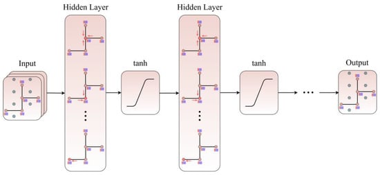
Figure 1.
The architecture of the GCN model.
We can simplify through the formula below:
where is the adjacency matrix, is its degree matrix, and and are its weight coefficients.
Based on the assumption , it is now possible to overcome the problem of overfitting and haphazard calculations during analysis.
Moreover, we introduced the renormalization trick to alleviate the problems of gradient anomalies in Equation (6):
where is the adjacency matrix with added self-connections, is the unit matrix, and is the degree matrix.
Then, the GCN model is constructed by stacking multiple convolutional layers, which can be expressed as follows:
where is the output of the -th layer, is the weight matrix, and is the activation function.
2.2. Attribute-Augmentation Unit
The gas injection rate (GIR) of the injector is modeled as a dynamic attribute . Afterward, the attribute augmentation cell (A-cell) receives the adjacency matrix , the production feature matrix , and the attribute matrix to make the final capacity prediction based on these three matrices, as shown in Figure 2.
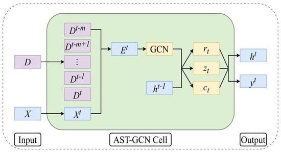
Figure 2.
The architecture of an AST-GCN cell.
Considering that the production state in a specific period is cumulatively influenced by the dynamics, therefore, a new augmented matrix can be obtained by combining which contains all the dynamic attributes and which contains the characteristics of production. The attribute augmentation cell is as follows:
2.3. Temporal Dependence Modeling
As a variant of recurrent neural networks, the GRU model not only captures trends but also describes temporal relationships. GRU works by using gating mechanisms to remember long-term information, and it is equally effective for a wide range of tasks. Compared to other algorithms, GRU has a simple structure, few parameters, and fast training capabilities. Therefore, GRU was chosen to determine the temporal dependence of the production data.
A key characteristic of GRU is that it is based on the cell state and two gates, which marks it apart from RNNs. The architecture of the RNN and GRU is shown in Figure 3. and denotes the reset gate and update gate, respectively, which can be described as Equations (9) and (10), respectively:
where is the weight matrix and is the bias matrix of the reset gate. is the weight matrix and is the bias matrix of the update gate. represents the output at time and is the input at time . is an activation function. We chose as the activation function. Subsequently, the new memory cell state can be obtained by Equation (11):
where is the weight matrix for the new memory cell state and is the bias matrix. The symbol is the Hadamard product.
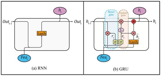
Figure 3.
The architecture of (a) RNN and (b) GRU.
The gate signal () ranges from 0 to 1. The closer the gating signal is to 1, the more data is remembered, and the closer to 0, the more is forgotten. Thus, one expression can control forgetting and input to produce an output () in Equation (12):
2.4. Attribute-Augmented Spatiotemporal Graph Convolutional Network
In this study, GCN and GRU are combined to build an AST-GCN model, which aims to capture spatiotemporal correlation on production data, as shown in Figure 4. The augmentation matrix is used as the input of the model , and the final prediction result is obtained in Equation (13):
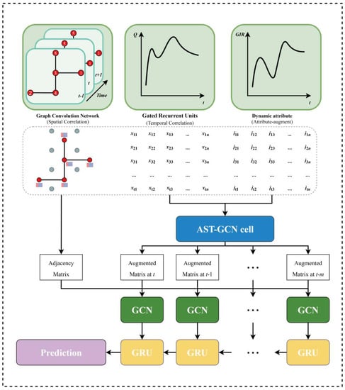
Figure 4.
The structure of AST-GCN in this paper.
The process of combining GCN and GRU for well network production forecasting is represented by Equations (14)–(17).
where is the graph convolution operation, and are learnable parameters. and are the true value and prediction value at time , represents the L2 regularization, and is a hyperparameter that controls the regularization rate.
3. Case Study
3.1. Workflow
The overall structure of this paper is shown in Figure 5. Based on the collected data, the data is preprocessed, including denoising, normalization, and splitting. Then, the proposed model is trained and optimized using the training sets until the set criteria are met. Finally, the trained model is used for prediction on the test set to verify the effectiveness and robustness of the proposed model. Each specific step in the flowchart is described in detail below.
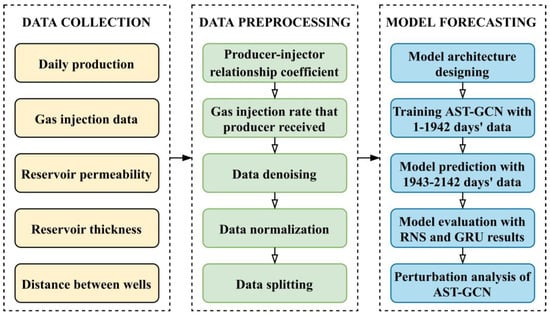
Figure 5.
Workflow of our proposed method.
3.2. Reservoir Background
Our target oil reservoir (Reservoir B) is in the Middle East and is a low-topographic tight carbonate reservoir with a small gas cap on the top and an oil-water transition zone on the lower side. The overall porosity of the B reservoir is between 12% and 17%, which is moderate to good. However, the average calculated core permeability is less than 5 mD, except for a few points in partitions BII and BIII, which exceed 10 mD and are less than 50 mD. The lower permeability is attributed to the blocking of the primary intergranular effective pore system caused by diagenesis. All production wells and water injection wells are 6-inch open-hole horizontal wells without any modification measures. The average length of a horizontal well is 4000 feet. The depth of each well is between 8920 feet and 9060 feet, which means that the maximum depth difference is only 140 feet. Yaser Ahmadi [48] carried out strict experimental research on a carbonate reservoir, and the author studied the impact of different driving mechanisms on oil recovery. Specifically, it was found that the associated gas had a higher recovery potential, which illustrates the priority of gas injection in the carbonate reservoir.
In this study, we selected five producers and seven gas injectors as the target well pattern. HC gas is injected into the target reservoir to increase production. For each injector, the target injection rate is 20,000 Mscf/day, and the target injection pressure is 5000 psi. It is sufficient to meet our needs using the production/injection data since 2006 when gas injection began.
3.3. Data Collection and Preprocessing
The following datasets are used, including the production and GIR data. The production data contains five producers’ raw production history from 1 February 2011 to 22 March 2017, as shown in Figure 6. The relation is modeled by a 5*5 adjacency matrix in Equation (19). The oil production time series of the selected wells were collected, and a feature matrix in a 2242*5 matrix was formed.
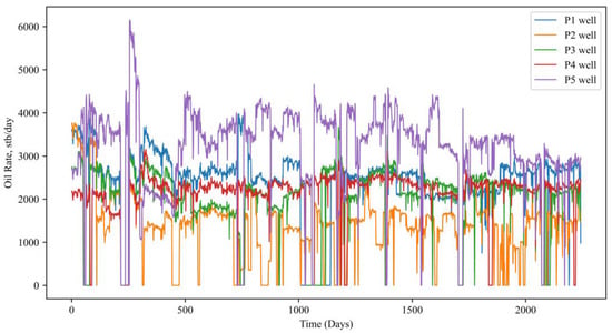
Figure 6.
The raw daily oil production series of five wells in a well pattern.
The gas injection rate of the gas injection well is a very important factor affecting production. Some traditional deep learning algorithms can also consider the gas injection rate of the adjacent wells, but these methods have limitations. Specifically, the gas injected by the gas injection well does not all flow to a certain producer but will flow to all the connected wells in different proportions. However, when the traditional deep learning method takes the gas injection rate of adjacent wells as the input feature, it can only consider a gas injection well’s overall gas injection rate rather than the gas injection rate data most relevant to the particular producer.
To better apply the gas injection data, this paper defines a coefficient named a producer–injector relationship coefficient to quantify the effect between the wells, which can be calculated by Equation (20).
Specifically, a 2242*5 matrix needs to be obtained, where the row represents the number of days, the column represents each production well, and the matrix value represents the gas injection rate received by a producer from adjacent gas injection wells at a specific time. Since a producer may be directly connected to a different number of injection wells, this paper believes that this value is jointly determined by the producer–injector relationship coefficient and the gas injection rate of all the adjacent gas injection wells.
The corresponding permeability parameters, reservoir thickness, and well distance can be obtained from geological data and have reference significance. Based on the calculated connection degree coefficient , combined with the GIR of the injection well obtained by statistics, the gas injection volume received by a production well on a certain day can be calculated by Equation (21), which is a 2242*5 matrix. As we can see in Equation (20), the sum of several centered on a production well should be one:
where represents the producer, represents the gas injectors connected with the producer, represents the number of producers, represents the average permeability between the production well and the adjacent gas injection well , mD, represents the average thickness of the reservoir between the production well and the adjacent gas injection well , m, and represents the distance between two wells, m.
represents the gas rate received in the -th producer from the connected gas injectors and is the gas injection rate of the -th injector. The producer–injector relationship coefficient calculated in this paper is shown in Figure 7. According to the results of the coefficient and the gas injection volume of the adjacent gas injection wells, we can comprehensively calculate the gas volume received by a production well on a certain day, which will be collected as a 2242*5 matrix.
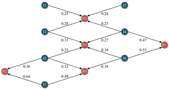
Figure 7.
The producer–injector relationship coefficient of the target well pattern in this study.
After data collection, we introduce the process of data preprocessing, including denoising, normalization, and splitting. First, we will introduce the process of data denoising. The Kalman filter is an optimal autoregressive data processing algorithm, which simply predicts the optimal value based on the existing measured values. Thus, we utilize the Kalman denoising method to remove noise from production data, thus smoothing the trend of the production data series. The average determination coefficient between the raw oil production and the denoised daily oil production is 0.9788, which is shown in Figure 8, indicating that the noise is effectively removed and the key information in the dataset is retained.
where is the system state, and is the control amount of the system. and are system parameters, and for multi-model systems, they are matrices. is the measurement value at time , is the parameter of the measurement system, and for a multi-measurement system, which is a matrix. and represent the process and measurement noise, respectively.
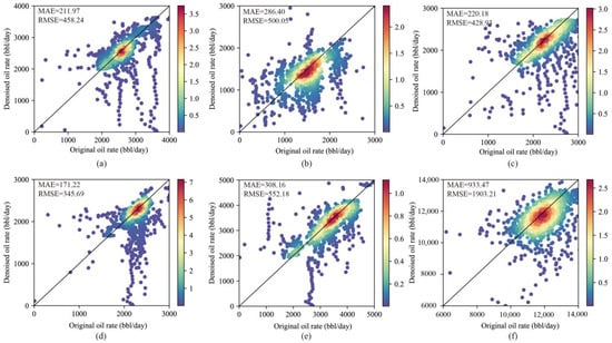
Figure 8.
The performance of Kalman filter: (a) P1 well; (b) P2 well; (c) P3 well; (d) P4 well; (e) P5 well; (f) well pattern.
Then, the Min-Max-Scaler was used to normalize the production characteristics, as shown in Equation (24). The data used in this study is divided into a training set and a test set with a ratio of 87:13; the first 87% of the data as a training set is used for training the hybrid model. The last 13% of the data as a testing set is used to evaluate the performance of the prediction.
is input variable after normalization.
3.4. Model Structure, Training, and Evaluation
To evaluate the prediction performance of the proposed model, four metrics, including RMSE, MAE, MedAE, and accuracy, are utilized to evaluate the prediction results. The specific formulas of the three evaluation indicators are as follows in Equations (25)–(27):
where is the -th actual value, is the -th predicted value, and is the number of samples in question.
In order to better compare the performance between the algorithms, the accuracy evaluation criteria are defined as Equation (28)–(30).
3.5. Comparison of Models
To further demonstrate the superiority of the AST-GCN model proposed in this paper, the AST-GCN model is compared with traditional RNS and GRU.
RNS: In this paper, we performed the 1942-day historical matching of target reservoirs, including five producers. The historical matching quality is shown in Figure 9. The oil production rate, water production rate, gas production rate, and GOR are all well-adjusted to actual values. Under these conditions, the numerical model of the reservoir can be used to predict oil production. During the prediction process, the injection rate is set to be consistent with the actual value, and the production rate is set to be controlled by the bottom hole pressure (BHP).
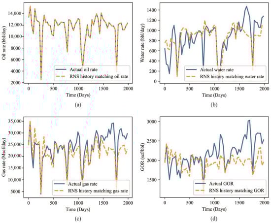
Figure 9.
RNS history matching performance of target area: (a) Oil rate; (b) Water rate; (c) Gas rate; (d) GOR rate.
GRU: For a fair comparison, this paper uses the gas injection volume of the adjacent wells as an additional input feature to predict the production of five producers in turn. Before formally applying the GRU model to predict well pattern production, it is necessary to verify the applicability of the GRU model. Based on the numerical simulation model, we selected a producer as the prediction object. After the data preprocessing steps described above, the production data in the first 1942 days were input into the GRU model. The architecture of the GRU model is shown in Table 2. The production prediction results and error analysis are shown in Figure 10 and Table 3. As shown in Table 3, the MedAE of GRU is 210.73, the MAE is 306.56, the RMSE is 515.15, and the accuracy is 86.72. From the production prediction results, it is clear that GRU can capture the dynamic characteristics. Therefore, the well prediction effect proves the applicability of the GRU model in production prediction.
Table 2.
The architecture of the GRU model proposed in this paper.
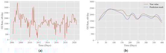
Figure 10.
The predictive performance of oil production using GRU model: (a) The raw data from the numerical model; (b) The prediction result.
Table 3.
Error analysis of the prediction performance.
4. Experimental Result
In this section, firstly, the production of five producers in a low-permeability carbonate reservoir in the Middle East will be predicted, and the results will be compared with GRU and RNS; secondly, the result of the well pattern production prediction will be compared with RNS which has the ability to predict the production of the well pattern. In addition, different degrees of Gaussian noises are added to the input features to verify the robustness of the hybrid model.
4.1. Comparison Results of Forecasting Performance
To validate the AST-GCN model’s performance in the production forecast, the RNS and GRU prediction results are compared to the ground truth, as shown in Figure 11. From this, the three models’ predicted trends are consistent with the daily oil production.
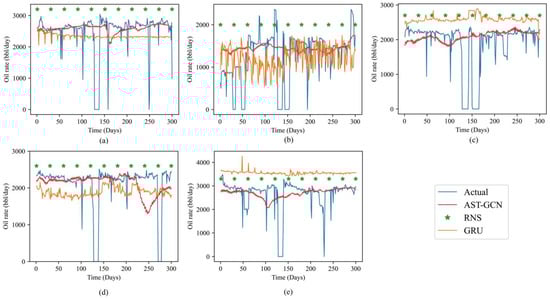
Figure 11.
The predictive performance of daily oil production using the different models: (a) P1 well; (b) P2 well; (c) P3 well; (d) P4 well; (e) P5 well.
The predicted results of RNS are generally much higher than the true value, and the trend is flat. This may be due to its inability to capture the changes in complex and variable production characteristics.
The prediction results of GRU are higher than the real value (such as P3, P5), some are lower (such as P1, P4), and some fluctuate greatly, and the law is difficult to judge. The architecture of the GRU makes the accuracy limited, and it could not be used for wells with more complex production changes (such as P2).
The AST-GCN prediction results show a higher degree of both trend and accuracy, which proves that the proposed hybrid model performs better in predicting oil production. For a visual comparison, the four evaluation criteria, MedAE, MAE, RMSE, and accuracy for the test set, are shown in Figure 12. In all the test wells, RNS and GRU had more errors than AST-GCN. The observations show that AST-GCN performs better in terms of accuracy and stability.
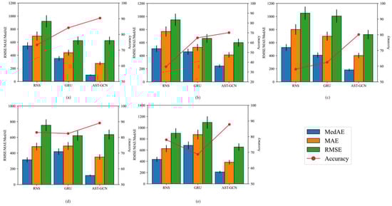
Figure 12.
Comparison of prediction accuracy: (a) P1 well; (b) P2 well; (c) P3 well; (d) P4 well; (e) P5 well.
For the P1 well, the MedAE of AST-GCN is 72.1% and 81.9% lower than GRU and RNS, respectively. The MAE of AST-GCN is 37.2% and 60.2% lower than GRU and RNS, respectively. The RMSE of AST-GCN is 0.1% and 32.1% lower than GRU and RNS, respectively. Similarly, the accuracy of AST-GCN is 7.2% and 23.2% higher than GRU and RNS, respectively.
For all five test wells, the mean MedAE of AST-GCN is 63.2% and 62.9% lower than that of GRU and RNS, respectively. The mean MAE is 37.3% and 44.6% lower than that of GRU and RNS. The mean RMSE is 16.1% and 28.9% lower than that of GRU and RNS. Similarly, the accuracy of AST-GCN is 15.9% and 35.8% higher than GRU and RNS, respectively.
4.2. Well Pattern Production Prediction Results
Although the previous prediction method includes RNS and GRU, GRU is a prediction of the production of a single well and cannot output the production of multiple wells simultaneously. AST-GCN and RNS boost the capacity to predict the production of all producers at once, which means that the entire well pattern production can be obtained. Prediction results for the well pattern using AST-GCN and RNS are shown in Figure 13. (5 producers). The evaluation indicators are shown in Table 4. For the production forecasting of the well pattern, the error value of AST-GCN is 41.2%, 64.2%, and 75.2% lower in RMSE, MAE, and MedAE compared with RNS, respectively. At the same time, the accuracy of AST-GCN in the well pattern prediction is 29.3% higher than RNS.
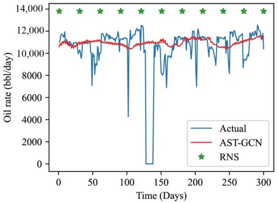
Figure 13.
The predictive performance of daily oil production in whole well pattern.
Table 4.
Performance comparison of different models for well pattern production forecasting.
Theoretically, the entire reservoir’s production may be predicted if the spatial distribution matrix, time-dimensional matrix of production, and gas injection can be obtained. On the one hand, the production forecast of the entire reservoir can be aggregated upwards to predict the total benefits of the reservoir; in addition, it can be allocated downwards to predict the economics of developing management units and developing single-well reservoirs, and hence, oilfield enterprises with a basis for making decisions regarding reservoir management can be obtained.
As mentioned above, AST-GCN performs very well in predicting five producing wells and predicting well pattern production. Therefore, it can be concluded that the model considering the production data, gas injection data, and spatial correlation has better prediction results than the RNS and GRU model. At the same time, the proposed hybrid model has also achieved satisfactory results in predicting the well pattern production, which fully proves that the proposed hybrid model has strong adaptability.
4.3. Perturbation Analysis Results
Different degrees of Gaussian noise was added to test the robustness, which follows a Gaussian distribution . Taking P2 well as an example, the experimental results obtained after adding noise to the production data are shown in Figure 14.
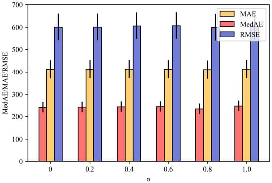
Figure 14.
Perturbation analysis (P2 well).
With the addition of different degrees of noise, it was found that the changes in the evaluation indicators of the P2 well were negligible. Compared with the ground truth, the average difference in MedAE was 3.3%, with a maximum of 8.7%. The average change in MAE was 0.4%, with a maximum of 0.9%. The average change in RMSE was 1.2%, with a maximum of 2.3%. Therefore, the model proposed in this paper has almost negligible changes in the evaluation indicators under different noise settings, which verifies the robustness of the AST-GCN model.
5. Discussion
This study aims to develop a new method that could simultaneously consider production data, gas injection data, and well patterns to obtain more accurate production predictions.
RNS is a common prediction method that can consider both the complex fluid flow process and output production of multiple wells simultaneously. However, the prediction of RNS depends on a lot of preparatory work in the early stage, and there are great uncertainties in preliminary geological research, so the accuracy of the model cannot be guaranteed.
GRU is a top-down modeling method based on neural networks. The GRU method can obtain more accurate prediction results than RNS. However, the GRU method is aimed at predicting the production of a single well and does not consider the interaction between adjacent producers.
To improve the accuracy of production prediction, a hybrid model named AST-GCN was proposed. The hybrid model presented in this paper has the following advantages: (1) The connectivity between adjacent wells can be considered, which broadens the limitations of single well production from the perspective of spatial distribution; (2) The gas injection rate of the adjacent wells can be considered as a dynamic attribute, which improves the learning ability of the hybrid model; (3) GRU is selected for time scale training because it boosts fewer parameters with faster speeds. However, compared with the single model, the hybrid model has more parameters, so more attempts are needed to adjust the parameters to achieve the best prediction state.
There are three main advantages of this study. First, the connection relationship between the producers is considered in the form of an adjacency matrix, which makes it possible to extract the spatial correlation from the data. The gas injection rate is split, and the most relevant gas injection data for a specific production well is obtained, which is used as a dynamic attribute to improve the prediction accuracy. Finally, all data used for model training and testing are actual production data from carbonate reservoirs in the Middle East, and it is expected that this study can be applied to actual reservoir management and development.
In the process of research, we also encountered some limitations. First, due to insufficient data, we excluded many important parameters, such as BHP and WHFP, which undoubtedly greatly impact production. Moreover, the producer–injector relationship coefficient defined in this paper is a constant value obtained based on geological data, and the reservoir parameters, such as permeability in the actual production process, will vary.
Based on the above statement, in future research work, the process of splitting the gas injection rate should be made more accurate and real. To improve the accuracy of predictions, more dynamic elements will be included in the attribute-augment matrix, such as permeability and choke size.
6. Conclusions
This work proposes a new framework based on AST-GCN and GRU for oil rate prediction. The main workflow includes data collection and preprocessing, data splitting, model establishing, and a comparison between different models. AST-GCN is used to capture the spatiotemporal patterns between each well from the input features, and GRU is used to achieve multi-well time series prediction. As an alternative method, it can provide an instructive value for future oil production. The proposed method is applied to a well pattern from a low-permeability carbonate reservoir in the Middle East to verify its effectiveness and robustness. The main conclusions are as follows:
- A hybrid model considering the production data, gas injection data, and spatial correlation is established, which eliminates the limitation that only single well productions can be predicted in previous studies.
- The injection and production data of five producers and seven gas injectors were collected for 2242 days. The producer–injector relationship coefficient was defined according to geological data, and the gas injection volume received by a certain producer was successfully calculated, which provides the foundation for the training of subsequent models.
- For fair evaluation, the AST-GCN model is compared with traditional RNS and GRU for single-well production prediction. The result shows that the error of AST-GCN is 63.2%, 37.3%, and 16.1% lower in MedAE, MAE, and RMSE, compared with GRU, respectively. Compared with RNS, AST-GCN is 62.9%, 44.6%, and 28.9% lower in MedAE, MAE, and RMSE. Similarly, the accuracy of AST-GCN is 15.9% and 35.8% higher than GRU and RNS, respectively.
- Similar to RNS, the AST-GCN model can forecast the production of the well pattern. The error of AST-GCN is 41.2%, 64.2%, and 75.2% lower in RMSE, MAE, and MedAE compared with RNS, while the accuracy of AST-GCN is 29.3% higher than RNS.
- Different degrees of Gaussian noise is added to the denoised data. Compared with the actual value, the average change in AST-GCN is 3.3%, 0.4%, and 1.2% in MedAE, MAE, and RMSE, and the model was found to be stable and robust from the perspective of the evaluation indicators.
- In the future, we will devote ourselves to establishing a method to quickly find the hyper-parameters in the modeling progress so as to improve the efficiency of building the hybrid model; other characteristics, such as pressure data, will be considered within the range of input characteristics in the future.
- According to the planned production of the development management unit, the downward distribution between the whole reservoir and the single well can be realized, which provides a basis for enterprise management decision-making.
Author Contributions
Conceptualization, M.G. and R.H.; methodology, C.W.; software, M.G.; validation, J.Y.; formal analysis, R.H.; investigation, R.H.; resources, C.W.; data curation, C.W.; writing—original draft preparation, M.G.; writing—review and editing, R.H.; visualization, X.Z.; supervision, B.L.; project administration, C.W. All authors have read and agreed to the published version of the manuscript.
Funding
This research was funded by National Natural Science Foundation of China (Grant No. 51974357).
Data Availability Statement
Data is unavailable due to privacy restrictions.
Conflicts of Interest
The authors declare that there are no conflicts of interest regarding the publication of this paper.
References
- Liu, W.; Liu, W.D.; Gu, J. Forecasting Oil Production Using Ensemble Empirical Model Decomposition Based Long Short-Term Memory Neural Network. J. Pet. Sci. Eng. 2020, 189, 107013. [Google Scholar] [CrossRef]
- Arnold, R.; Anderson, R. United States Geological Survey Bulletin 357: Preliminary Report on Coalinga Oil District, Fresno and Kings Counties; Government Printing Office: Washington, DC, USA, 1908.
- Arps, J.J. Analysis of Decline Curves. Trans. AIME 1945, 160, 228–247. [Google Scholar] [CrossRef]
- Tomomi, Y. Non-Uniqueness of History Matching. In Proceedings of the SPE Asia Pacific Conference on Integrated Modelling for Asset Management, Yokohama, Japan, 25 April 2000; p. SPE-59434-MS. [Google Scholar]
- Li, Y.; Sun, R.; Horne, R. Deep Learning for Well Data History Analysis. In Proceedings of the SPE Annual Technical Conference and Exhibition, Calgary, AB, Canada, 30 September 2019; p. D011S008R002. [Google Scholar]
- Song, X.; Liu, Y.; Xue, L.; Wang, J.; Zhang, J.; Wang, J.; Jiang, L.; Cheng, Z. Time-Series Well Performance Prediction Based on Long Short-Term Memory (LSTM) Neural Network Model. J. Pet. Sci. Eng. 2020, 186, 106682. [Google Scholar] [CrossRef]
- Rahuma, K.M.; Mohamed, H.; Hissein, N.; Giuma, S. Prediction of Reservoir Performance Applying Decline Curve Analysis. IJCEA 2013, 4, 74–77. [Google Scholar] [CrossRef]
- Lee, K.; Lim, J.; Yoon, D.; Jung, H. Prediction of Shale-Gas Production at Duvernay Formation Using Deep-Learning Algorithm. SPE J. 2019, 24, 2423–2437. [Google Scholar] [CrossRef]
- Al-Qasim, A.; AlDawsari, M.A. Comparison Study of Asphaltene Precipitation Models Using UTCOMP, CMG/GEM and ECLIPSE Simulators. In Proceedings of the SPE Oil and Gas India Conference and Exhibition, Mumbai, India, 4 April 2017; p. D011S001R005. [Google Scholar]
- Ostojic, J.; Rezaee, R.; Bahrami, H. Production Performance of Hydraulic Fractures in Tight Gas Sands, a Numerical Simulation Approach. J. Pet. Sci. Eng. 2012, 88–89, 75–81. [Google Scholar] [CrossRef]
- Xu, F.; Yu, W.; Li, X.; Miao, J.; Zhao, G.; Sepehrnoori, K.; Li, X.; Jin, J.; Wen, G. A Fast EDFM Method for Production Simulation of Complex Fractures in Naturally Fractured Reservoirs. In Proceedings of the SPE/AAPG Eastern Regional Meeting, Pittsburgh, PA, USA, 10 October 2018; p. D043S007R001. [Google Scholar]
- Ahmadi, Y.; Hassanbeygi, M.; Kharrat, R. The Effect of Temperature and Injection Rate during Water Flooding Using Carbonate Core Samples: An Experimental Approach. Iran. J. Oil Gas Sci. Technol. 2016, 5, 18–24. [Google Scholar] [CrossRef]
- Wang, Q.; Wan, J.; Mu, L.; Shen, R.; Jurado, M.J.; Ye, Y. An Analytical Solution for Transient Productivity Prediction of Multi-Fractured Horizontal Wells in Tight Gas Reservoirs Considering Nonlinear Porous Flow Mechanisms. Energies 2020, 13, 1066. [Google Scholar] [CrossRef]
- Wilson, K.C.; Durlofsky, L.J. Optimization of Shale Gas Field Development Using Direct Search Techniques and Reduced-Physics Models. J. Pet. Sci. Eng. 2013, 108, 304–315. [Google Scholar] [CrossRef]
- Ahmadi, Y.; Aminshahidy, B. Inhibition of Asphaltene Precipitation by Hydrophobic CaO and SiO2 Nanoparticles during Natural Depletion and CO2 Tests. Int. J. Oil Gas Coal Technol. 2018, 24, 394. [Google Scholar] [CrossRef]
- Liu, W.; Zhang, Z.; Chen, J.; Jiang, D.; Wu, F.; Fan, J.; Li, Y. Feasibility Evaluation of Large-Scale Underground Hydrogen Storage in Bedded Salt Rocks of China: A Case Study in Jiangsu Province. Energy 2020, 198, 117348. [Google Scholar] [CrossRef]
- Nwaobi, U.; Anandarajah, G. Parameter Determination for a Numerical Approach to Undeveloped Shale Gas Production Estimation: The UK Bowland Shale Region Application. J. Nat. Gas Sci. Eng. 2018, 58, 80–91. [Google Scholar] [CrossRef]
- Clarkson, C.R.; Williams-Kovacs, J.D.; Qanbari, F.; Behmanesh, H.; Heidari Sureshjani, M. History-Matching and Forecasting Tight/Shale Gas Condensate Wells Using Combined Analytical, Semi-Analytical, and Empirical Methods. J. Nat. Gas Sci. Eng. 2015, 26, 1620–1647. [Google Scholar] [CrossRef]
- El-Banbi, A.H.; Wattenbarger, R.A. Analysis of Commingled Tight Gas Reservoirs. In Proceedings of the SPE Annual Technical Conference and Exhibition, Denver, CO, USA, 6 October 1996; p. SPE-36736-MS. [Google Scholar]
- Hutahaean, J.J.; Demyanow, V.; Christie, M.A. Impact of Model Parameterisation and Objective Choices on Assisted History Matching and Reservoir Forecasting. In Proceedings of the SPE/IATMI Asia Pacific Oil & Gas Conference and Exhibition, Nusa Dua, Indonesia, 20 October 2015; p. SPE-176389-MS. [Google Scholar]
- Hutahaean, J.; Demyanov, V.; Christie, M. Many-Objective Optimization Algorithm Applied to History Matching. In Proceedings of the 2016 IEEE Symposium Series on Computational Intelligence (SSCI), Athens, Greece, 6–9 December 2016; IEEE: Athens, Greece, 2016; pp. 1–8. [Google Scholar]
- Hutahaean, J.; Demyanov, V.; Christie, M.A. On Optimal Selection of Objective Grouping for Multiobjective History Matching. SPE J. 2017, 22, 1296–1312. [Google Scholar] [CrossRef]
- Huang, R.; Wei, C.; Wang, B.; Yang, J.; Xu, X.; Wu, S.; Huang, S. Well Performance Prediction Based on Long Short-Term Memory (LSTM) Neural Network. J. Pet. Sci. Eng. 2022, 208, 109686. [Google Scholar] [CrossRef]
- Li, J.; Wan, J.; Wang, T.; Yuan, G.; Jurado, M.J.; He, Q. Leakage Simulation and Acoustic Characteristics Based on Acoustic Logging by Ultrasonic Detection. Adv. Geo-Energy Res. 2022, 6, 181–191. [Google Scholar] [CrossRef]
- Yang, Y.; Liu, S. Estimation and Modeling of Pressure-Dependent Gas Diffusion Coefficient for Coal: A Fractal Theory-Based Approach. Fuel 2019, 253, 588–606. [Google Scholar] [CrossRef]
- Clemens, T.; Viechtbauer-Gruber, M. Impact of Digitalization on the Way of Working and Skills Development in Hydrocarbon Production Forecasting and Project Decision Analysis. In Proceedings of the SPE Reservoir Evaluation & Engineering, Virtual, 1 December 2020; p. D011S007R002. [Google Scholar]
- Nwachukwu, A.; Jeong, H.; Pyrcz, M.; Lake, L.W. Fast Evaluation of Well Placements in Heterogeneous Reservoir Models Using Machine Learning. J. Pet. Sci. Eng. 2018, 163, 463–475. [Google Scholar] [CrossRef]
- Huang, R.; Wei, C.; Wang, B.; Li, B.; Yang, J.; Wu, S.; Xiong, L.; Li, Z.; Lou, Y.; Gao, Y.; et al. A Comprehensive Machine Learning Approach for Quantitatively Analyzing Development Performance and Optimization for a Heterogeneous Carbonate Reservoir in Middle East. In Proceedings of the SPE Eastern Europe Subsurface Conference, Kyiv, Ukraine, 23 November 2021; p. D012S001R001. [Google Scholar]
- Lee, K.; Kim, S.; Choe, J.; Min, B.; Lee, H.S. Iterative Static Modeling of Channelized Reservoirs Using History-Matched Facies Probability Data and Rejection of Training Image. Pet. Sci. 2019, 16, 127–147. [Google Scholar] [CrossRef]
- Udegbe, E.; Morgan, E.; Srinivasan, S. From Face Detection to Fractured Reservoir Characterization: Big Data Analytics for Restimulation Candidate Selection. In Proceedings of the Annual Technical Conference and Exhibition, San Antonio, TX, USA, 11 October 2017; p. D031S030R002. [Google Scholar]
- Wan, J.; Jiang, S.; Xia, Y.; Li, J.; Li, G. Numerical Model and Program Development of Horizontal Directional Drilling for Non-Excavation Technology. Environ. Earth Sci. 2021, 80, 579. [Google Scholar] [CrossRef]
- Huang, R.; Wei, C.; Li, B.; Xiong, L.; Yang, J.; Wu, S.; Gao, Y.; Liu, S.; Zhang, C.; Lou, Y.; et al. A Data Driven Method to Predict and Restore Missing Well Head Flow Pressure. In Proceedings of the International Petroleum Technology Conference, Riyadh, Saudi Arabia, 23 February 2022; p. D032S154R004. [Google Scholar]
- Huang, R.; Wei, C.; Yang, J.; Xu, X.; Li, B.; Wu, S.; Xiong, L. Quantitative Analysis of the Main Controlling Factors of Oil Saturation Variation. Geofluids 2021, 2021, 1–12. [Google Scholar] [CrossRef]
- Wei, C.; Huang, R.; Ding, M.; Yang, J.; Xiong, L. Characterization of Saturation and Pressure Distribution Based on Deep Learning for a Typical Carbonate Reservoir in the Middle East. J. Pet. Sci. Eng. 2022, 213, 110442. [Google Scholar] [CrossRef]
- Azamifard, A.; Rashidi, F.; Ahmadi, M.; Pourfard, M.; Dabir, B. Toward More Realistic Models of Reservoir by Cutting-Edge Characterization of Permeability with MPS Methods and Deep-Learning-Based Selection. J. Pet. Sci. Eng. 2019, 181, 106135. [Google Scholar] [CrossRef]
- Etienam, C. 4D Seismic History Matching Incorporating Unsupervised Learning. In Proceedings of the SPE Europec featured at 81st EAGE Conference and Exhibition, London, UK, 5 June 2019; p. D031S005R005. [Google Scholar]
- Huang, R.; Wei, C.; Li, B.; Yang, J.; Wu, S.; Xu, X.; Ou, Y.; Xiong, L.; Lou, Y.; Li, Z.; et al. Prediction and Optimization of WAG Flooding by Using LSTM Neural Network Model in Middle East Carbonate Reservoir. In Proceedings of the Abu Dhabi International Petroleum Exhibition & Conference, Abu Dhabi, United Arab Emirates, 15 November 2021; p. D011S012R003. [Google Scholar]
- Li, X.; Ma, X.; Xiao, F.; Xiao, C.; Wang, F.; Zhang, S. Time-Series Production Forecasting Method Based on the Integration of Bidirectional Gated Recurrent Unit (Bi-GRU) Network and Sparrow Search Algorithm (SSA). J. Pet. Sci. Eng. 2022, 208, 109309. [Google Scholar] [CrossRef]
- Zhao, L.; Song, Y.; Zhang, C.; Liu, Y.; Wang, P.; Lin, T.; Deng, M.; Li, H. T-GCN: A Temporal Graph Convolutional Network for Traffic Prediction. IEEE Trans. Intell. Transport. Syst. 2020, 21, 3848–3858. [Google Scholar] [CrossRef]
- Du, E.; Liu, Y.; Cheng, Z.; Xue, L.; Ma, J.; He, X. Production Forecasting with the Interwell Interference by Integrating Graph Convolutional and Long Short-Term Memory Neural Network. SPE Reserv. Eval. Eng. 2022, 25, 197–213. [Google Scholar] [CrossRef]
- Yin, H.; Yang, L.; Xu, H.; Wan, J. Adaptive Convolutional Neural Network for Large Change in Video Object Segmentation. IET Comput. Vis. 2019, 13, 452–460. [Google Scholar] [CrossRef]
- Tian, Y. Artificial Intelligence Image Recognition Method Based on Convolutional Neural Network Algorithm. IEEE Access 2020, 8, 125731–125744. [Google Scholar] [CrossRef]
- Chang, J.; Wang, L.; Meng, G.; Zhang, Q.; Xiang, S.; Pan, C. Local-Aggregation Graph Networks. IEEE Trans. Pattern Anal. Mach. Intell. 2019, 42, 2874–2886. [Google Scholar] [CrossRef]
- Wu, R.; Kamata, S. K(3)-Sparse Graph Convolutional Networks for Face Recognition. In Proceedings of the 2018 15th International Conference on Control, Automation, Robotics and Vision (ICARCV), Singapore, 30 May 2018; pp. 174–179. [Google Scholar]
- Bruna, J.; Zaremba, W.; Szlam, A.; LeCun, Y. Spectral Networks and Locally Connected Networks on Graphs. arXiv 2013, arXiv:1312.6203. [Google Scholar]
- Kipf, T.N.; Welling, M. Semi-Supervised Classification with Graph Convolutional Networks. arXiv 2016, arXiv:1609.02907. [Google Scholar]
- Feng, F.; He, X.; Wang, X.; Luo, C.; Liu, Y.; Chua, T.-S. Temporal Relational Ranking for Stock Prediction. ACM Trans. Inf. Syst. 2019, 37, 30. [Google Scholar] [CrossRef]
- Ahmadi, Y.; Mansouri, M. Using New Synthesis Zirconia-Based Nanocomposites for Improving Water Alternative Associated Gas Tests Considering Interfacial Tension and Contact Angle Measurements. Energy Fuels 2021, 35, 16724–16734. [Google Scholar] [CrossRef]
Disclaimer/Publisher’s Note: The statements, opinions and data contained in all publications are solely those of the individual author(s) and contributor(s) and not of MDPI and/or the editor(s). MDPI and/or the editor(s) disclaim responsibility for any injury to people or property resulting from any ideas, methods, instructions or products referred to in the content. |
© 2022 by the authors. Licensee MDPI, Basel, Switzerland. This article is an open access article distributed under the terms and conditions of the Creative Commons Attribution (CC BY) license (https://creativecommons.org/licenses/by/4.0/).