Article

Comparison of Corrected and Uncorrected Enthalpy Methods for Solving Conduction-Driven Solid/Liquid Phase Change Problems

by
Andreas König-Haagen
* and
Gonzalo Diarce
ENEDI Research Group, Department of Energy Engineering, Faculty of Engineering of Bilbao, University of the Basque Country UPV/EHU, 48013 Bilbao, Spain
*
Author to whom correspondence should be addressed.
Energies 2023, 16(1), 449; https://doi.org/10.3390/en16010449
Submission received: 17 November 2022 / Revised: 19 December 2022 / Accepted: 26 December 2022 / Published: 31 December 2022

Abstract

:
The numerical study of solid/liquid phase change problems represents a large and ongoing field of research with many applications. These simulations should run as fast and accurately as possible. Therefore, proceeding from previous work and findings from the literature, this study investigates enthalpy methods for solving solid/liquid phase change problems. The relationship between temperature and enthalpy is strongly non-linear and requires special treatment; iteratively corrected methods, as well as approaches that do not correct the temperature/enthalpy relationship at all or only once per time step, were considered for a one-dimensional test problem. Based on the results of this study, two solvers can be recommended, the so-called optimum approach and a simple explicit method; both provide accurate results. The explicit method is easy to program, but the optimum approach allows larger time steps and is, therefore, faster. The influence of several parameters was investigated. The mesh resolution strongly influenced the accuracy and the computational speed, and the time step size barely influenced the accuracy but did affect the computational speed. An artificial melting temperature range influenced the accuracy but had hardly any influence on the simulation speed. Higher-order time discretization schemes were not superior compared to the first-order implicit optimum approach.

1. Introduction

Solving solid/liquid phase change problems numerically is a widely performed task in the fields of latent heat thermal energy storage [1], welding [2], continuous casting [3] and food processing [4], among others. In these types of problems, the most common approaches to describe the transition from solid to liquid or vice versa are the enthalpy methods, also called fixed grid methods [5]. As stated by Furzeland [6], who compares such different approaches as front-tracking methods with the enthalpy method, the latter is very attractive as it has no computational overheads, is easy to program and can be used for complex geometries and materials with a mushy phase change. However, it needs a fine mesh to achieve highly accurate solutions.
Within the family of the enthalpy method, many approaches have been developed over the years [4,5,7,8,9] to solve the challenging coupling between enthalpy and temperature. A possible classification of these enthalpy methods is shown in Figure 1 with typical examples. Following this classification, the methods can be divided into explicit and implicit approaches as well as corrected and uncorrected approaches, which refer to the coupling of the temperature and the enthalpy. The implicit corrected solvers can be further subdivided into methods that apply only one correction per time step and iterative methods, which update the temperature and the enthalpy until convergence.
Several comparisons are available in the literature considering the accuracy and speed of different enthalpy methods. Bertrand et al. [10] and Gobin et al. [11] compare various methods from different research groups; however, as there is no exact solution available for the 2D melting problem, they only studied a comparison of the results they obtained among each other. The attained results are generally similar. A comparable attempt was made by Pointner [12], who included the simulation time in the performed evaluation. Which solver performed best depended on the time step and mesh resolution. Tamma and Namburu [13] analyzed explicit and implicit enthalpy methods for the finite element method; they found that the explicit methods are faster since no update of the mass matrix is necessary. Mauder et al. [14] compared different methods in MATLAB for accuracy, simulation time, and the applicability of parallelization. They stated that the effectiveness of the methods depends on the problem under study.
When it comes to iterative methods (which update the temperature/enthalpy relation after solving the energy equation and reiterate the two steps as necessary), it has been repeatedly shown [5,15,16,17,18,19] that the optimum approach developed by Swaminathan and Voller [17,19], or its source-based counterpart [18] (which performs identically to the optimum approach [5]) have advantages over other methods. Pham [20] developed an apparent heat capacity method with a single posterior correction step that uses an implicit time-stepping with three time levels (a similar method was developed by Comini et al. [21]). However, the idea of the correction step can be applied to lower-order methods as well. The method was compared to iteratively corrected and non-corrected approaches. For the same level of accuracy, it performed two to three times faster than the best of the other methods studied [20]. Pham’s method [20] was also compared with the optimum approach by Pham [22], Voller [5] and Al-Saadi and Zhai [23]. The latter also developed a hybrid method that switches from Pham’s method to the optimum approach when at least one cell is changing phase. Pham’s method appears to be faster than the optimum approach for small time steps but produces oscillations for large time steps [5,22]. These studies, however, were performed for a limited parameter space; did not include, for instance, explicit approaches for comparison; or were performed for building simulations only [23].
Moreover, even for isothermal phase change, some methods rely on an arbitrary melting temperature range instead of a single melting point. Changing the temperature enthalpy relation from the real one can have a large effect on the results of numerical models [24]. Hence, the following questions arise: how should it be modeled, linear or with a smoothed function? How significant is the error that comes with the implementation of an arbitrary melting range? Moreover, melting or solidification simulations are nowadays more and more embedded in larger or more complex simulation problems. These can be system simulations that include other components [25,26] or multiphysics simulations that include further physical aspects such as close contact melting [27,28], or additional components like a heat exchanger and a heat transfer fluid [29,30]. In any of these cases, the maximum time step might be dictated by aspects other than the temperature/enthalpy coupling, and it would be beneficial to know how a simple explicit method performs in comparison to implicit ones. For the case of system simulations, even the time-stepping scheme might be optimized for other parts of the model, e.g., in MATLAB Simulink with a selection of ordinary differential equation (ODE) solvers and implementing iterative methods might be restricted.
Bearing the abovementioned research gaps in mind, the main objective of this paper is to enlarge the knowledge of the numerical solution of solid/liquid phase change problems by addressing the following questions:
  • How does the optimum approach perform compared to non-iterative methods in terms of accuracy and speed?
  • How do the mesh, the time step and an artificial melting temperature range affect the accuracy of the methods?
  • How do the mesh, the time step and an artificial melting temperature range influence the calculation speed?
  • Does using a smoothed temperature/enthalpy curve for isothermal phase changes give some advantages for solvers relying on an apparent heat capacity?
  • Does the use of higher-order methods for the time discretization give any benefit?
  • Which methods are appropriate when implementing the solid/liquid phase change in solvers with an automated time step control—like the ODE solvers in MATLAB? Moreover, how do they perform compared to the other solvers studied?
  • Does linearizing the diffusion term of the energy equation instead of the transient term (i.e., the optimum approach) give any benefits?
To meet the objective, a simple 1D conduction-driven case, known as the Lamé–Clapeyron–Stefan problem [31,32], was solved with different solvers for a variation of several parameters, such as the time step size and the mesh resolution, among others, leading to about 6000 simulations. By also describing the procedure of each solver in detail, this paper will not only help to choose the right solver but also program it.

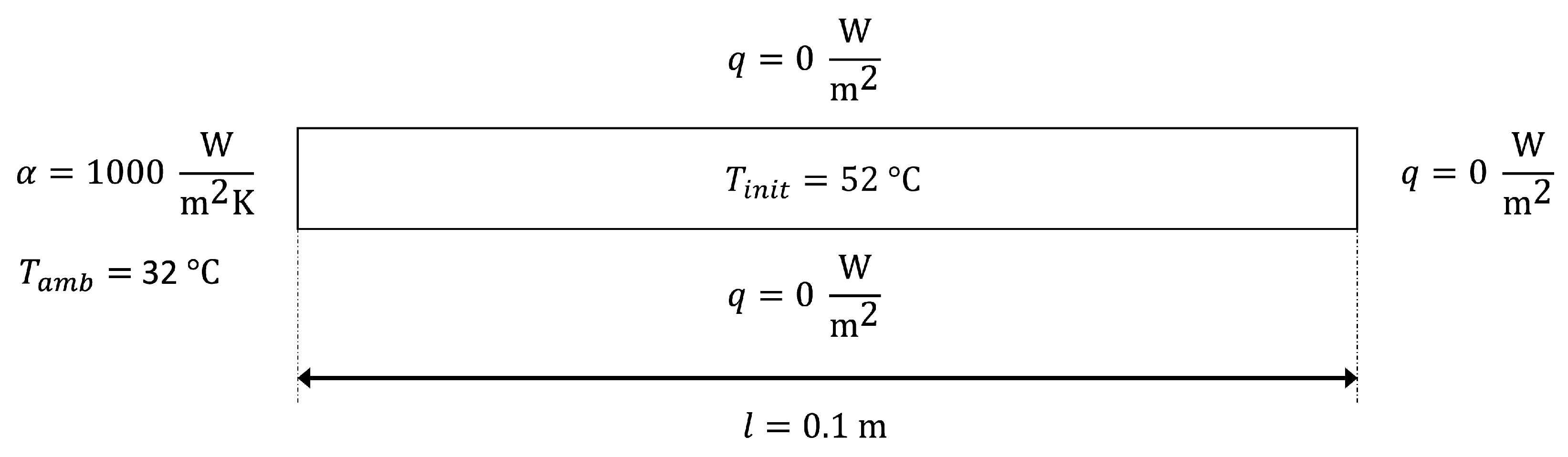
2. Problem Statement

In this section, the physical problem and the governing equations are described first. Then the numerical methods, the parameter variation and the error calculation are presented in detail.

2.1. Physical Problem and Governing Equations

As depicted in Figure 2, the physical problem consists of a one-dimensional slab of generic material, initially in a homogenous liquid state, which starts to solidify at t = 0 due to a convective boundary condition at the left-hand side. The other boundary of the sample is adiabatic.
Table 1 shows the material properties of the generic material used and lists the initial and boundary conditions. All material properties are assumed to be constant and identical for the solid and liquid states. Later on, the numerical results are compared to a benchmark solution. To validate the benchmark solver, a similar problem is used that has an analytical solution [33]. The whole procedure is described in detail in Section 3.
The general equation describing the heat transfer in the considered domain is presented in Equation (1), with the enthalpy H , the temperature T , the time t , and the heat conductivity λ . Depending on the solver applied, Equation (1) is either directly discretized or first reformulated.
H t = λ 2 T x 2

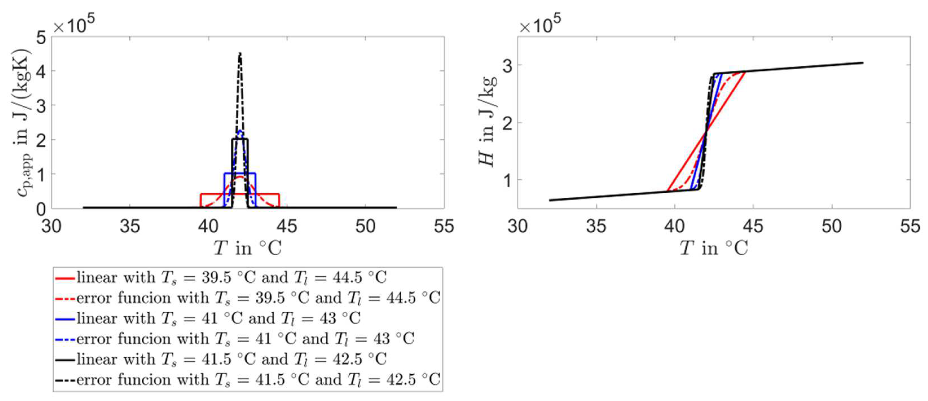
2.2. Implementation of the Temperature/Enthalpy Relation

Based on thermodynamics, the melting/solidification phase change for a pure material is a first-order transition. This means that there is a discontinuity in the enthalpy/temperature relation when the phase change occurs. However, since some c p , a p p -based solvers do not allow the implementation of a step-function, or may perform much worse with a step-function, the temperature/enthalpy curves with an artificial melting temperature range T m are implemented as well. Even though there exist plenty of possible slopes for c p , a p p over temperature—like triangular-shaped or sine-based [34]—we limit the number of variations. Therefore, only two kinds of curves are considered: (i) a linear one; and (ii) one based on an error function. In Figure 3, the slopes of several curves are shown as examples.
The definition of c p , a p p for the linear case is described with Equation (2):
c p , a p p = c p T T s c p + L T l T s T s < T < T l c p T l T
and for the error function, it is Equation (3):
c p , a p p = c p + L · 4 · e 4 T T m T l T s 2 T l T s · π
For the linear case, H as a function of T can be described with Equation (4):
H = c p · T T T s c p · T + L T l T s · T T s T l T s T s < T < T l c p · T + L T l T
and for the error function, we have Equation (5):
H = c p · T + L · 1 0.5 · e r f c 4 · T T m T l T s
To describe T as a function of H , Equation (6) is used for the linear case:
T = H c p H H s T s + H H s L · T l T s H s < H < H l T l + H H l c p H l H
There is no analytical inverse error function, but there exists a built-in MATLAB function. This function, however, is quite slow, so an optimized look-up table was generated prior to the simulations, which was then called during the simulations.

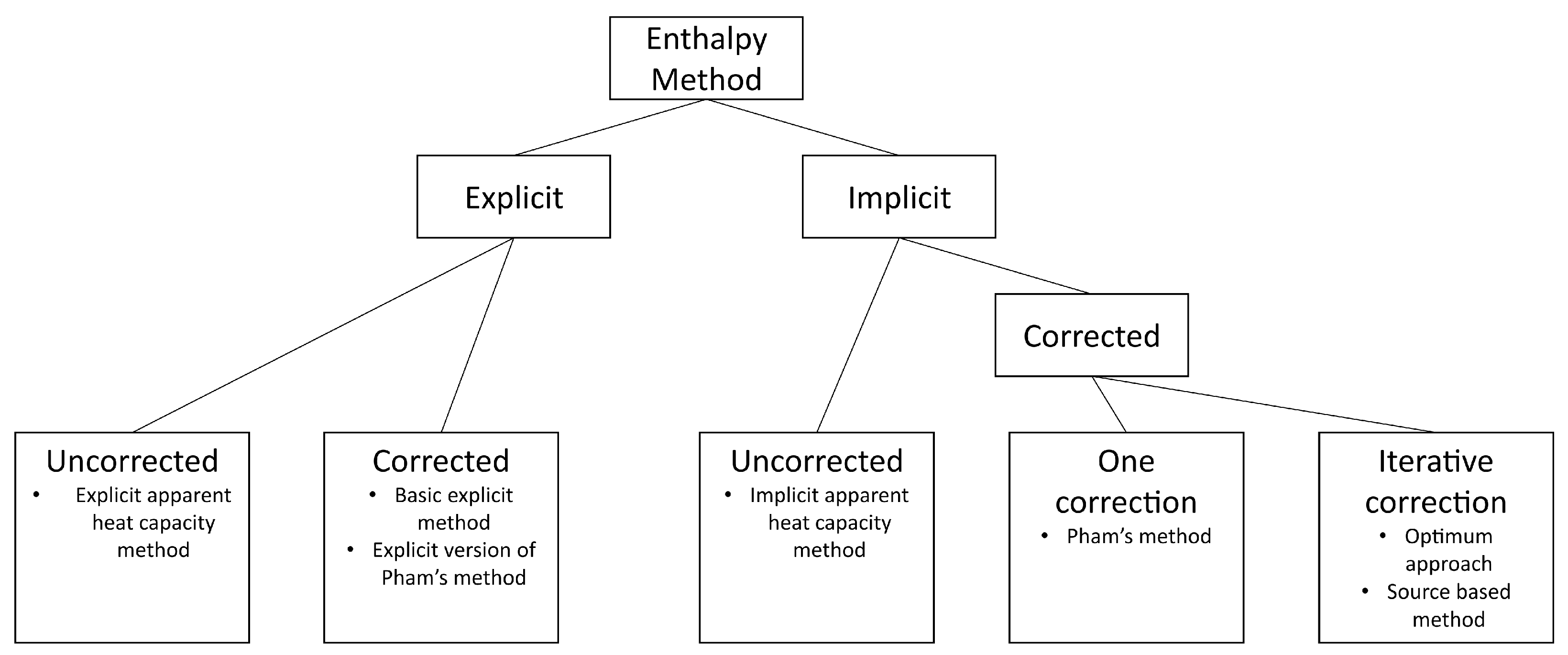
2.3. Numerical Methods

To address the research questions formulated in the introduction, several solvers are programmed in MATLAB R2020a. These solvers can be categorized by the following characteristics:
  • Correcting the temperature/enthalpy relation
    Uncorrected solvers
    Corrected solvers, the correction is performed once
    Iterative solvers, the correction is performed iteratively until a convergence criterion is reached
  • Slope of the temperature/enthalpy relation during phase change
    Linear function
    Error function
  • Time stepping
    Fixed-step explicit
    Fixed-step implicit
    Fixed-step Crank–Nicolson
    Variable step solver (ode15s solver)
In Table 2, an overview of all the solvers used is provided, together with their identifiers. For all solvers, the finite volume method is applied for spatial discretization, which is performed with a second-order scheme. In the following sections (Section 2.3.1, Section 2.3.2, Section 2.3.3, Section 2.3.4, Section 2.3.5 and Section 2.3.6), the procedure of the solvers is described and the pertinent equations are provided. More information on the solvers described in Section 2.3.1, Section 2.3.2, Section 2.3.3 and Section 2.3.4 can be found in the literature [5].

2.3.1. Basic Explicit Method (Corrected)

The procedure for the T/H-lin-expl solver is straightforward: Equation (1) is discretized, put in matrix form, and solved to calculate the new enthalpy field H n e w (see Equation (7)):
H n e w = H o l d + A c o e f · T o l d + R B
The right-hand side of Equation (7) is exclusively formed by known variables, which allows for a direct solution. After H n e w is calculated, T o l d for the next time step is determined by Equation (6), provided in Section 2.2. At the end of each time step, H o l d is updated by H n e w and the boundary conditions ( R B ) and the coefficient matrix ( A ¯ c o e f ) is updated if needed as well. The solver proceeds as follows:
  • Solve Equation (7)
  • Update T o l d and H o l d , as well as A ¯ c o e f and R B , if the material properties or the boundary conditions change
  • Go to the next time step
To optimize the calculation speed, A ¯ c o e f is implemented as a sparse matrix in MATLAB.

2.3.2. Apparent Heat Capacity Methods (Uncorrected)

For the cp-app-lin-expl, cp-app-lin-impl, cp-app-erf-expl, and cp-app-erf-impl solvers, Equation (1) needs to be reformulated by means of the relation c p , a p p T t = H t , to:
ρ c p , a p p T t = λ 2 T x 2
Equation (8) is then discretized and put in matrix form. For the explicit solvers, Equation (9) is obtained, which can be directly solved as all the variables on the right-hand side are known.
T n e w = T o l d + A ¯ c o e f · T o l d + R B
For the implicit solvers, it yields:
T n e w = A ¯ c o e f \ T o l d + R B
with the MATLAB intern operator “matrix left-divide \ ”. As c p , a p p changes with the temperature, A ¯ c o e f is not constant and needs to be updated after each time step. It was found that using triplets to build up a new sparse matrix each time step is the fastest update method. The procedure of the solver is as follows:
  • Determine c p , a p p and build A ¯ c o e f
  • Calculate T n e w with Equation (9) (explicit solvers) or Equation (10) (implicit solvers)
  • Go to the next time step

2.3.3. Apparent Heat Capacity Methods (Corrected)

For the corrected apparent heat capacity methods (cp-app-1xcorr-lin-expl, cp-app-1xcorr-lin-impl, cp-app-1xcorr-erf-expl and cp-app-1xcorr-erf-impl), Equation (8) is discretized following steps 1 and 2 detailed in Section 2.3.2. Then, a correction of T n e w is performed. To do so, a corresponding new enthalpy ( H n e w ) is calculated by Equation (11):
H n e w = H o l d + c p , a p p T n e w T o l d
Afterward, T n e w is updated via the temperature/enthalpy Equation (6) for the linear case or with the help of a look-up table for the error function case. Thus, the solver procedure is as follows:
  • Determine c p , a p p and build A ¯ c o e f
  • Calculate a preliminary T n e w with Equation (9) (explicit solvers) or Equation (10) (implicit solvers)
  • Calculate H n e w with Equation (11)
  • Update T n e w with Equation (6) or a look-up table.
  • Go to the next time step

2.3.4. Optimum Approach (Iteratively Corrected)

The core of the optimum approach solvers (opti-lin-impl, opti-lin-CN, opti-erf-impl and opti-erf-CN) is a Newton linearization of the enthalpy with respect to the iteration steps. This linearization is performed via Equation (12):
H k + 1 = H k + c p , a p p , k · T k + 1 T k
where H k + 1 and T k + 1 are the enthalpy and the temperature of the new iteration step and H k and T k are the enthalpy and temperature of the previous iteration step. As for the final iteration step, it is fulfilled: H k + 1 = H n e w , and the linearization from Equation (12) is included in the semi-discretized version of Equation (1), which leads to Equation (13):
ρ H k H o l d t + ρ c p , a p p , k T k + 1 * T k t = λ 2 T x 2
After Equation (13) is solved for T k + 1 * , H k + 1 is determined with Equation (12). Then, the temperature is updated to T k + 1 , either with Equation (6) for the linear case, or with the help of a look-up table for those solvers using the error function. If the difference between T k + 1 and T k + 1 * is smaller than a given threshold, the solution is considered converged; otherwise, T k and H k are updated and Equation (13) is solved again. This procedure is repeated until convergence. Two important aspects of Equation (13) are: (i) for the first iteration step H k = H o l d and (ii) at convergence T k + 1 * T k , this implies that the first term is not present at the first iteration step and the second term vanishes when convergence is reached. The optimum approach solvers are implemented either with an implicit Euler scheme or with the Crank–Nicolson scheme; the difference is only visible in the discretization of the diffusion term. The matrix equation looks like Equation (10), but here R B includes the additional known parts from the left-hand side of Equation (13) and the parts from the diffusion term corresponding to the old-time step for the Crank–Nicolson solvers as well. The single steps of the solver are:
  • Determine c p , a p p , k and build A ¯ c o e f
  • Calculate T k + 1 * with Equation (10)
  • Calculate H k + 1 with Equation (12)
  • Update T n e w with the Equation (6) or the look-up table.
  • Calculate the residual ( T k + 1 T k + 1 * )
  • Update H k and T k
  • Depending on the obtained residual value, go to step 1 or the next time step

2.3.5. Linearized Diffusion Term (Iteratively Corrected)

This solver (lin-diff-lin-impl) is similar to the optimum approach; however, instead of H in the transient term, T is linearized in the diffusion term. The linearization is performed by Equation (14).
T k + 1 = T k + H k + 1 H k c p , a p p , k
Semi-discretizing Equation (1) and implementing the linearization for the implicitly formulated diffusion term yields Equation (15):
ρ H k + 1 * H o l d t λ 2 T k x 2 + λ 2 H k c p , a p p , k x 2 = λ 2 H k + 1 c p , a p p , k x 2
The given Equation (15) is then put in matrix form and solved for H k + 1 * (Equation (16)):
H k + 1 * = A ¯ c o e f \ H o l d + R B
where all the known variables can be found in R B . Afterward, T k + 1 is determined with Equation (17):
T k + 1 = T k + H k + 1 * H k c p , a p p , k
The enthalpy is then updated with Equation (4) and the residual ( H k + 1 H k + 1 * ) is checked, which determines whether another iteration needs to be performed or not. At convergence H k + 1 * H k , and therefore, the two diffusion terms involving H vanish when converged. The procedure of the solver reads:
  • Determine c p , a p p , k and build A ¯ c o e f ;
  • Calculate H k + 1 * with Equation (16);
  • Calculate T k + 1 with Equation (17);
  • Update H k + 1 with Equation (4);
  • Calculate the residual H k + 1 H k + 1 * ;
  • Update H k and T k ;
  • Depending on the obtained residual value, go to step 1 or the next time step.

2.3.6. The ODE Solvers

To use the ODE solver from MATLAB, the method of lines [35] is applied to the corresponding equations described above. This results in a system of transient ODE for every solver, which is then handled by the MATLAB ode15s solver. Compared to other ODE solvers from MATLAB (ode45, ode23, ode113, ode23s, ode23t, ode23tb), the ode15s solver performed best on average. Therefore, only the results for the ode15s solver are shown below. The implementations involved, the pertinent equations and additional information can be found in the following list:
  • T/H-lin-ODE:
    Equation (1) is implemented semi-discretized, and T is updated with Equation (6)
  • cp-app-lin-ODE:
    Equation (8) is implemented semi-discretized, and c p , a p p is determined by Equation (2)
  • cp-app-erf-ODE:
    Equation (8) is implemented semi-discretized, and c p , a p p is determined by Equation (3)
  • cp-app-1xcorr-lin-ODE:
    Equation (8) is implemented semi-discretized, c p , a p p is determined by Equation (2) and the correction is performed with Equations (6) and (11).
  • cp-app-1xcorr-erf-ODE:
    Equation (8) is implemented semi-discretized, c p , a p p is determined by Equation (3) and the correction is performed with Equation (11) and a look-up table.

2.4. Parameter Variation

A study was performed to gain knowledge of the influence of certain parameters on the numerical accuracy of the solvers. The mesh number of nodes and the width of the artificial melting temperature range T m were varied for every solver described in Section 2.3 (Table 2). The time step size t was also varied for all solvers except the ODE solvers. For the latter, the relative tolerance was varied instead. The time step size was varied according to the relation t / t s t a b , where t s t a b is the time step size for which the explicit stability criterion equals 1. The adopted parameter values are detailed in Table 3. The simulations were carried out using one kernel of an Intel® Xeon® Gold 6252 CPU @ 2.10 GHz (Intel Corporation, Santa Clara, CA, USA) processor.

2.5. Error Calculation

The error was calculated for the phase front position and the final temperature distribution. In both cases, the simulation results were compared to a benchmark solution described in Section 3. For the phase front position, the absolute error ( ε i ) and the relative error ( ε i rel ) were calculated for every time step ( i ) with Equations (18) and (19). The absolute error regarding the final temperature field ( ε j T ) was calculated with Equation (20) for every node ( j ) . When there is no reference node at the same position as T s i m j , an interpolation was performed to define the reference value.
ε i = X i sim X i ref
ε i rel = X i sim X i ref X i ref
ε j T = T j sim T x j ref
For all errors regarding the phase front position, mean values were calculated as well. These are defined in Equations (21)–(23) for ε i , ε i rel and ε j T , respectively.
ε mean = i = 1 i = n t X i sim X i ref · 1 n t
ε mean rel = i = 1 i = n t X i sim X i ref X i ref · 1 n t
ε mean T = j = 1 j = n x T j sim T x j ref · 1 n x
The evaluation of the results was performed based on the error of the phase front position while ε mean T was applied only to random samples to check the validity.

3. Validation and Benchmark Solution

To analyze the error of the different solvers, the simulation results were compared to a benchmark solution, which was validated against analytical results beforehand. The analytical results were not used directly for benchmarking as they refer to a semi-infinite problem, which would require an unwieldy, long simulation domain in the numerical model.
The benchmark solution was obtained with the T/H-lin-expl solver and was compared with the analytical solution of a Lamé–Clapeyron–Stefan problem [33] with a convective boundary condition to validate it and check the mesh independency. The validation case is identical to the benchmark case except for the convective boundary condition, which is time-dependent, and the simulation domain, which is 1 m long in the validation case (for the exact conditions of the benchmark case and the parameter variation, see Section 2.1 and Section 2.4). For validation purposes, the error of the phase front position as a function of the mesh number of cells is presented in Figure 4. The error with finer meshes decreases below 10−6 m, so the solver is considered successfully validated. For the benchmark solution, the finest mesh resolution studied for the validation (20,000 nodes per meter) was used, which rendered 2000 nodes as the length of the benchmark simulation domain is 0.1 m. The maximum number of nodes for the variational simulations was 500, significantly lower than those used for the benchmark.

4. Results

In the following, the results are presented. Section 4.1 contains results analyzing the tested solvers in general. Section 4.2 deals with the influence of the varied parameters. A comparison of explicit and implicit methods is undertaken in Section 4.3 and in the final Section 4.4, the number of iterations needed for the optimum approach is studied.

4.1. General Results

Figure 5 shows ε mean rel plotted over the simulation time for all solvers and variations. At every plot, preferable simulations can be found on the lower left front, while simulations on the right are slow and simulations on the top are not accurate enough. Overall, the optimum approach solvers perform best in terms of simulation time and accuracy, followed by T/H-lin-expl and cp-app-1xcorr solvers. For these solvers, the smaller T m is, the smaller the minimum of ε mean rel . When it comes to the uncorrected cp-app solvers and the lin-diff-lin-impl solver, the mentioned trend is the other way around, and for the ODE solvers, no clear trend is visible. The optimum approach and the T/H-lin-expl solvers always result in a ε mean rel value below 10%, and its minimum is less than 0.01%. The simulation time varies between 10−4 and 104 s, but a ε mean rel lower than 0.01% can already be achieved with a simulation time of about 1 s.
When comparing the optimum approach solvers in more detail in terms of ε mean rel and the simulation time (see Figure 6), the following can be noted: (i) there are no large differences in the simulation times and errors between the tested implementations, (ii) the linear implementation performs somewhat faster than the error function for the same accuracy and (iii) the implicit Euler discretization outperforms the Crank–Nicolson approach for ε mean rel values from 1 to 10% and for values lower than 0.01%. In between, the Crank–Nicolson approach is faster.
An analysis of the different ODE solvers shows that there are some distinctive differences in their performance (see Figure 7). However, the cp-app-ODE and the cp-app-1xcorr-ODE solvers perform very similarly, which indicates that the correction has no significant effect here. Acceptable ε mean rel values can be achieved with all ODE implementations, but the T/H-lin-ODE solver needs the least simulation time for a given ε mean rel below 10% and, on average, the T/H-lin-ODE solver gives smaller ε mean rel than the other ODE solvers. Moreover, small T m lead to high ε mean rel for the cp-app-ODE and the cp-app-1xcorr-ODE solvers, and on the contrary, they lead to low ε mean rel for T/H-lin-ODE solver.
This section on general results is concluded with a study that addresses the question of how many simulations with a T m 0.1 give ε mean rel smaller than 1%. This question is of particular practical interest as it reveals under which conditions the solvers give realistic results, even though the threshold for “realistic” results was set arbitrarily to ε mean rel smaller than 1%. For every solver tested, these results can be seen in Figure A2 in the Appendix A, dependent on the mesh and the time step (or the error tolerance for the ODE solvers). Most importantly, all corrected methods (including T/H-lin-expl and T/H-lin-ODE), except the lin-diff-lin-impl solver, give ε mean rel smaller 1% for a broad field of parameters for T m 0.1 . All other solvers perform considerably worse. When it comes to implicit methods, the optimum approach solver performs most accurately and gives ε mean rel 1 % only for a mesh with 10 nodes and 20 nodes, and at the same time t / t stab 72 (Euler scheme) or t / t stab 144 (Crank–Nicolson approach). The uncorrected cp-app solvers and the lin-diff-lin-impl solver give ε mean rel larger than 1% for most cases, only for small t and a large number of nodes can an accurate result be achieved. The ODE solvers applying an apparent heat capacity only give accurate results for fine tolerances and meshes.

4.2. Influence of the Varied Parameters

In this section, the influence of the artificial melting temperature range ( T m ) , the number of nodes and the time step size ( t ) on ε mean rel is studied primarily for the most accurate solvers, namely the optimum approach solvers and the T/H-lin-expl solver. The influence of T m on ε mean rel is depicted in Figure 8. On average, ε mean rel decreases for the smaller T m . The minimum values of ε mean rel are very similar for all solvers shown and decrease from more than 10−2 for T m 1   K to 10−4 for a T m of 0 K. Finally, it can be noted that T m affects the maximum of ε mean rel much less than the minimum of ε mean rel .
For comparison, Figure A1 in the Appendix A shows the same results as Figure 8, but for the cp-app solvers without correction. Especially for small T m values, the cp-app solvers without correction give much larger ε mean rel .
The influence of the mesh resolution on ε mean rel is presented in Figure 9 for the optimum approach solvers and the T/H-lin-expl solver. The minimum of ε mean rel decreases by about two orders of magnitude for finer meshes for all solvers shown; while, on the contrary, the maximum and the mean of ε mean rel are only slightly influenced by the mesh.
In Figure 10, the influence of the time step size on ε mean rel is shown. Compared to the influence of the number of nodes and T m , the influence of t / t stab is smaller. As long as t / t stab 10 , there is practically no influence of the time step size on ε mean rel . For t / t stab > 10 , an increase of ε mean rel can be noted (for optimum approach solvers with an implicit Euler time-stepping scheme first, a decrease occurs for the minimum of ε mean rel after which an increase can be seen). Moreover, the increase is only small for all the solvers shown, even for the largest time steps studied, which refer to t / t stab = 216 , the minimum values of ε mean rel are still below 0.1%.

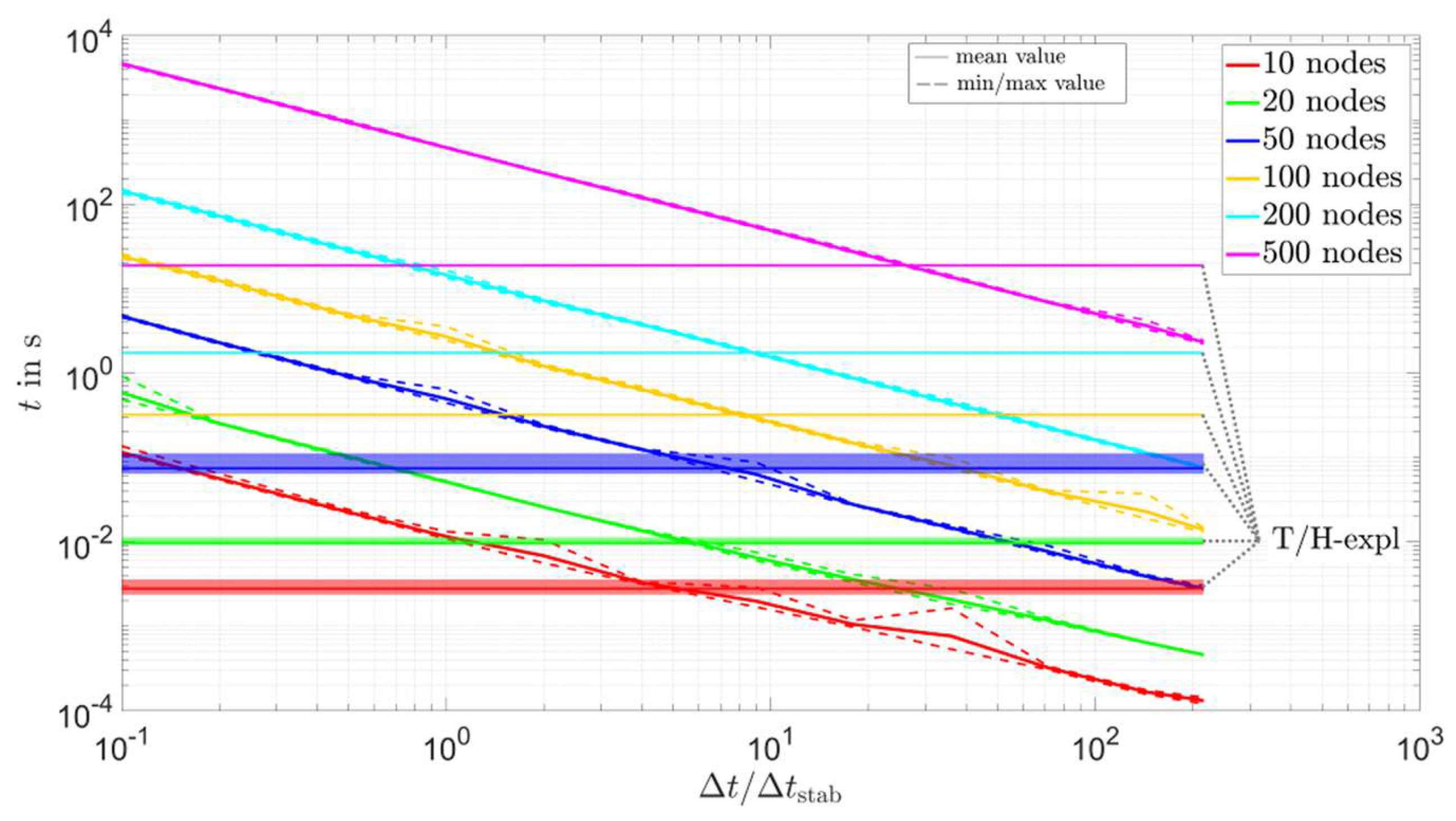
4.3. Implicit vs. Explicit Approaches

In this section, the value of t / t stab required for certain implicit solvers (optimum approach solvers and cp-app-1xcorr-impl solvers) to be faster than the basic explicit solver (T/H-lin-expl solver) is assessed. The cited implicit solvers were chosen as they give acceptable results in terms of accuracy. These results are listed in Table 4, while more detailed information can be found in Figure A3, Figure A4, Figure A5, Figure A6, Figure A7 and Figure A8 in the Appendix A. The minimum of the necessary t / t stab ranges between 2.5–4, and the maximum ranges between 7–25, depending on the solver. For the opti-lin solvers, the maximum of the needed t / t stab is lower than for the opti-erf and cp-app-1xcorr-impl solvers. Overall, the necessary t / t stab value increases with finer mesh resolutions. For the opti-erf-impl solver, there are some simulations with a larger t / t stab than listed in Table 4 that still lead to simulations slower than the T/H-lin-expl solver with a t / t stab = 1 .
From Figure A3, Figure A4, Figure A5, Figure A6, Figure A7 and Figure A8 in the Appendix A, it can also be seen that varying the number of nodes from 10 to 500 increases the simulation time for the optimum approach solvers and cp-app-1xcorr-impl solvers by about four orders of magnitude. When t / t stab is increased from 0.1 to 216, the simulation time is reduced by about three orders of magnitude. In contrast, T m has little influence on the simulation time.

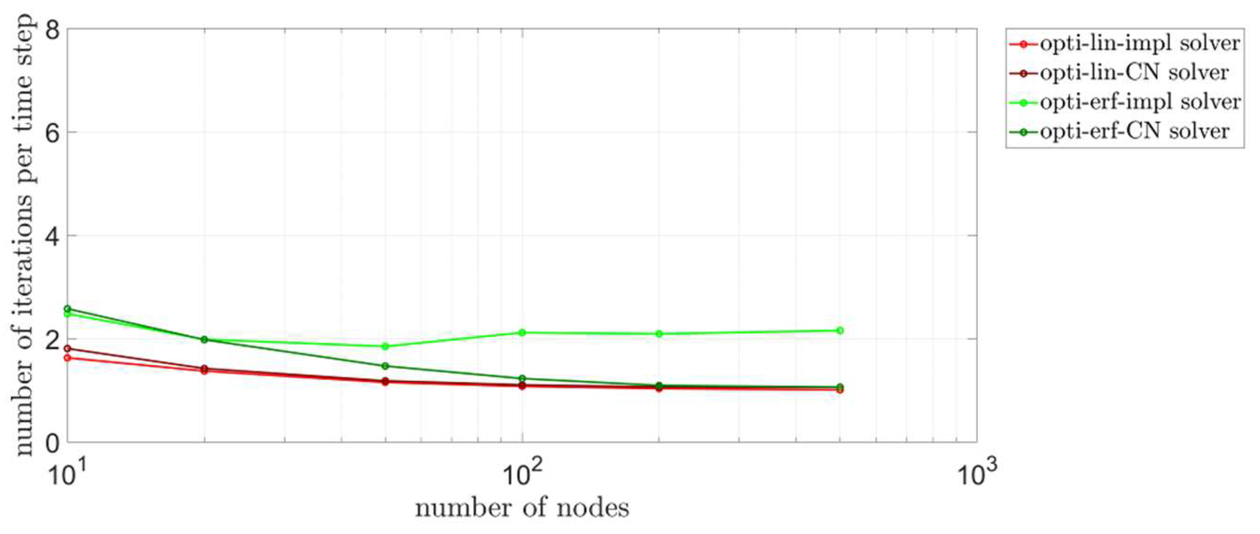
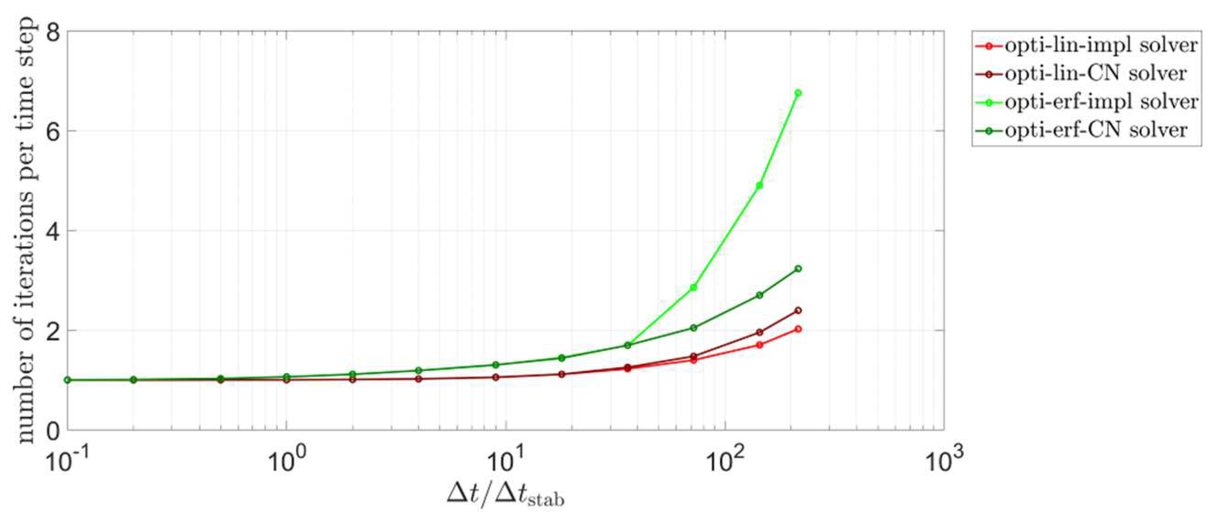
4.4. Iterations of the Optimum Approach Solvers

The number of iterations is also of great interest for iterative methods because it is independent of the computer used and gives information about how often additionally implemented features would need to be calculated. Therefore, the number of iterations per time step is analyzed next for the optimum approach solvers. In Figure 11, the average number of iterations per time step is plotted over T m . The average is less than two iterations per time step, apart from the opti-erf-impl solver at T m = 0   K , where the average is almost five iterations per time step. For all solvers shown, except the opti-erf-impl solver, T m does not considerably influence the number of iterations. Furthermore, choosing the Crank–Nicolson scheme or the implicit Euler scheme makes almost no difference for the number of iterations, except for the opti-erf solvers at T m = 0   K .
The number of iterations per time step decreases for a larger number of nodes for all optimum solvers, aside from the opti-erf-impl solver, which is only slightly influenced by the number of nodes (see Figure 12). If the mesh consists of 100 or more nodes, all optimum solvers except the opti-erf-impl solver need almost the same number of iterations.
As long as t / t stab 1 , all optimum solvers need a similar number of iterations (see Figure 13). For larger t / t stab , the solvers applying an error function need more iterations than the solvers with a linear function. The solvers using a Crank–Nicolson scheme need slightly (linear) or distinctly (error function) more iterations for very large t / t stab than the solvers using the implicit Euler scheme.

5. Discussion

Based on the results presented in Section 4, the research questions stated in the introduction will now be discussed. Some important aspects regarding the analyzed solvers are additionally commented on. The questions raised earlier and their answers are:
  • How does the optimum approach perform compared to non-iterative methods in terms of accuracy and speed?
  • The optimum approach led to the fastest simulations of the tested methods while still maintaining high accuracy. The basic explicit method (with the T/H-lin-expl solver) and, for certain parameter values, the apparent heat capacity method with one correction (cp-app-1xcorr solvers without the ODE solvers) also gave accurate results within an acceptable simulation time.
  • How do the mesh, the time step, and an artificial melting temperature range affect the accuracy of the methods?
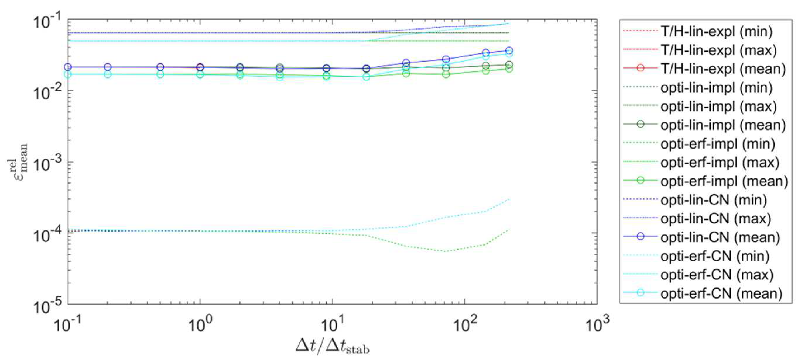
  • For the most accurate solvers (optimum approach and T/H-lin-expl), the mesh and using an artificial melting temperature range had a large effect on the accuracy. For example, by increasing the number of nodes from 10 to 500, the minimum value of ε mean rel was reduced by about two orders of magnitude. If no artificial melting temperature range was implemented, the minimum of ε mean rel was about 10−4; while, for a melting temperature range of 1 K, the minimum of ε mean rel increased to about 10−2. On the contrary, the influence of t / t stab was much smaller. Up to a t / t stab value of 10, there was a negligible influence on ε mean rel . For the largest time steps tested ( t / t stab = 216 ), the minimum of ε mean rel was only distinctive below 10−3.
  • How do the mesh, the time step and an artificial melting temperature range influence the calculation speed?
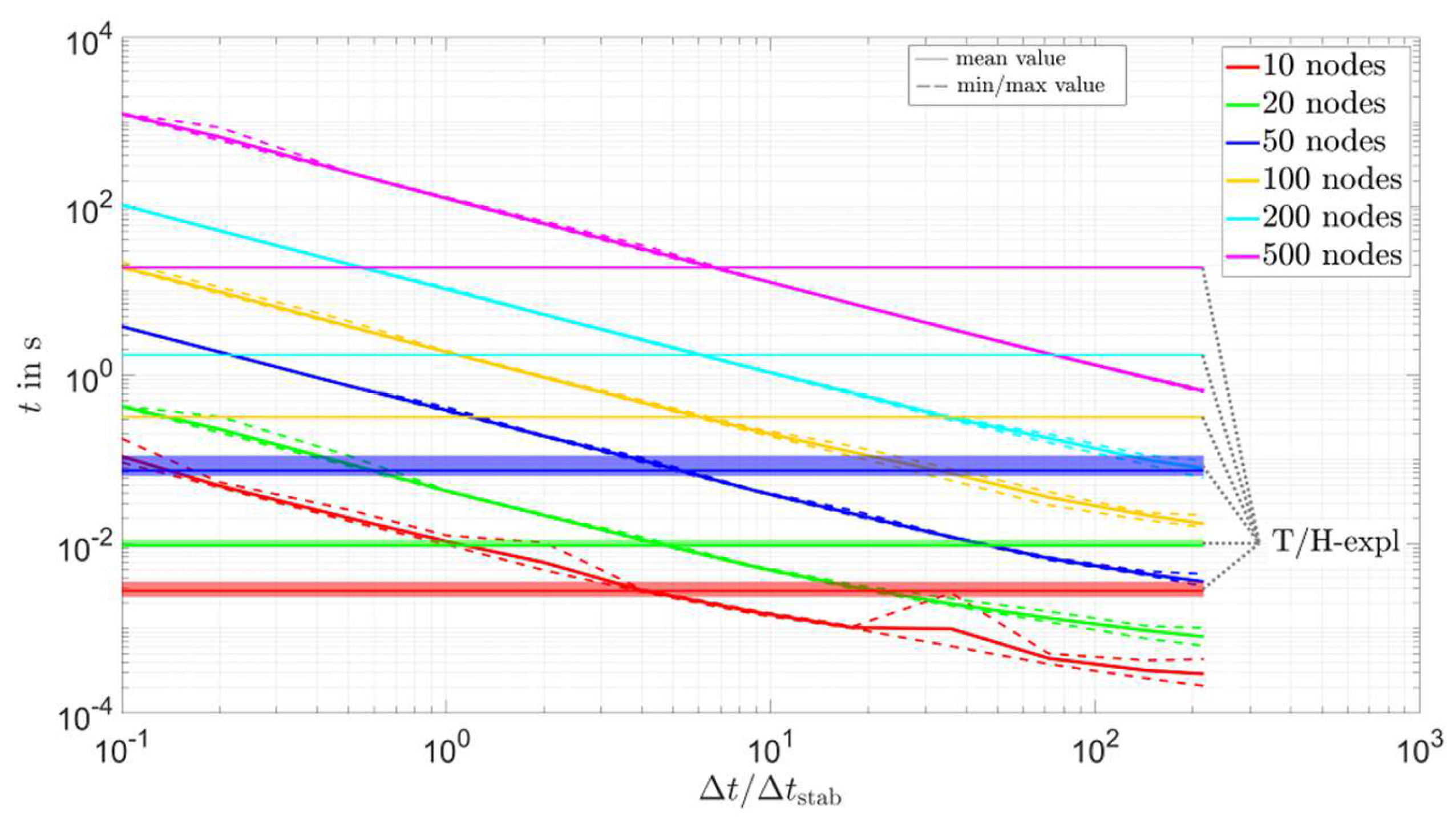
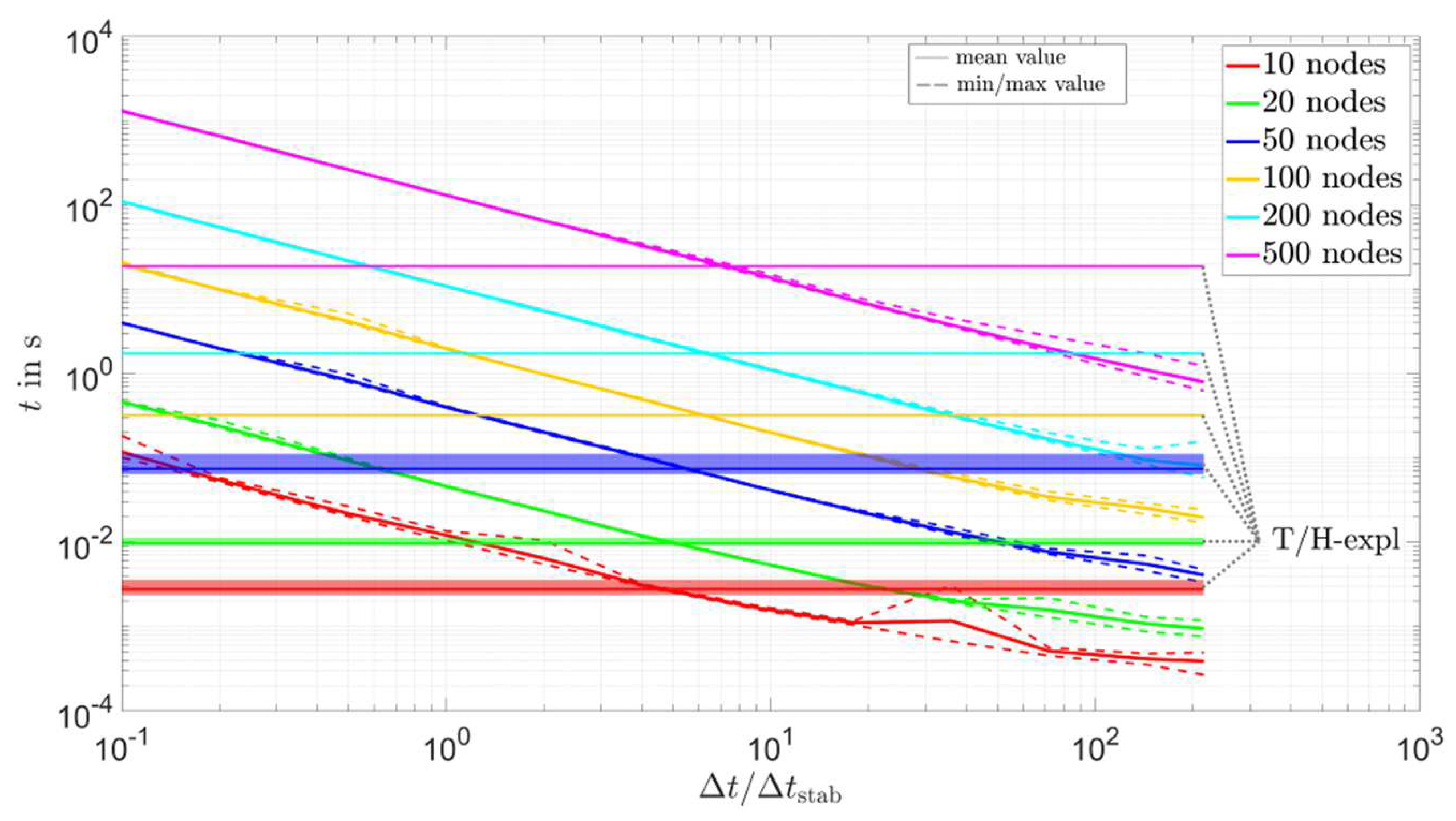
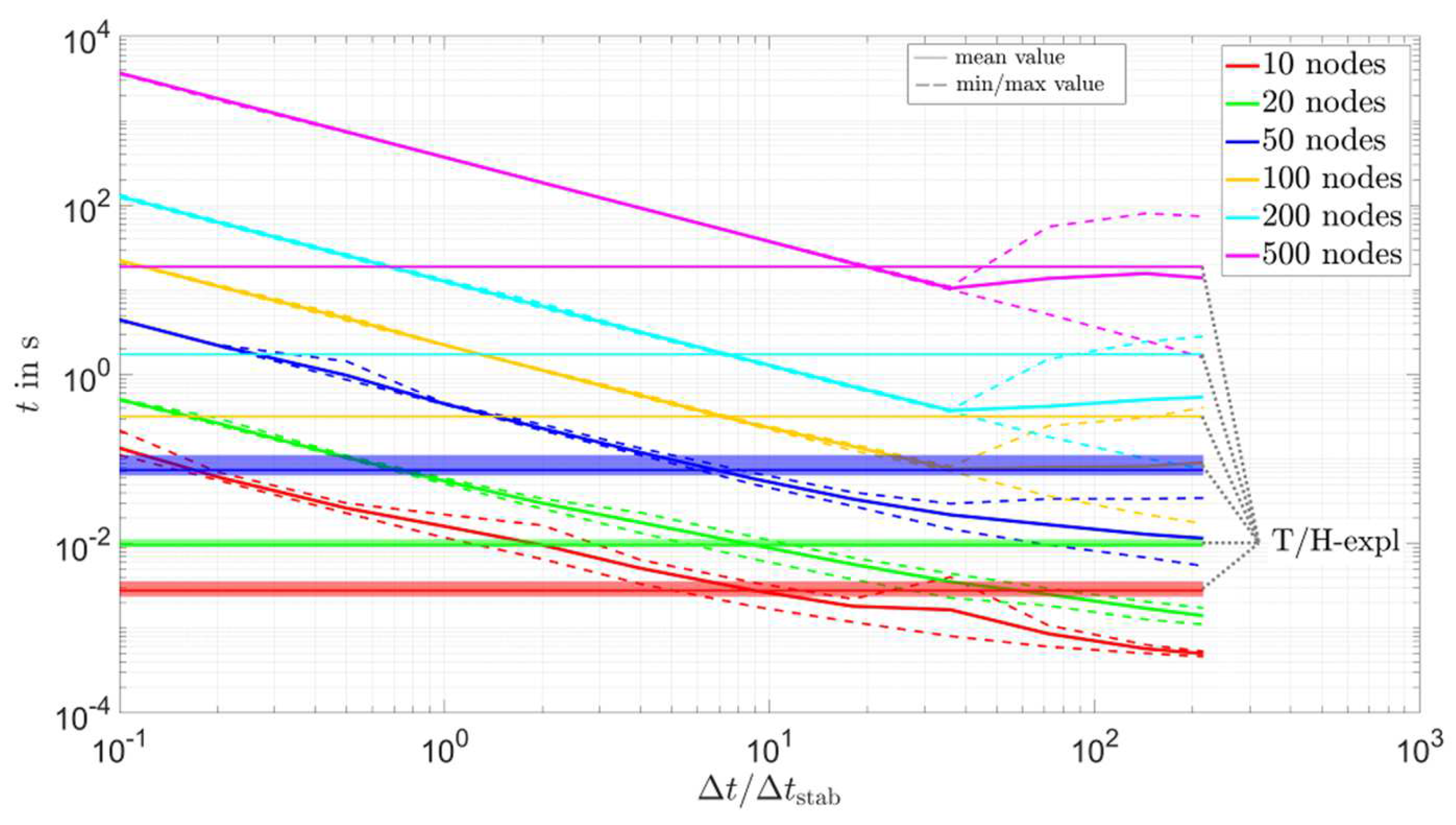
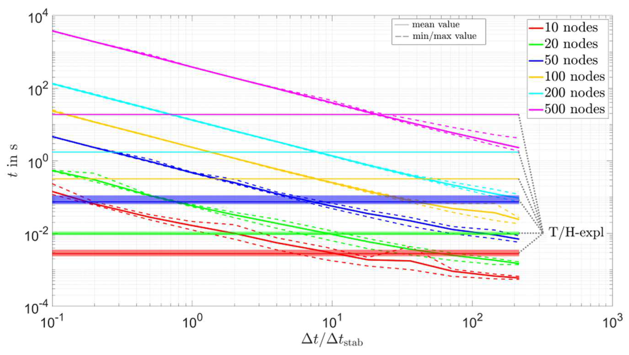
  • For the implicit solvers with acceptable accuracy (optimum approach and cp-app-1xcorr-impl solvers), the number of nodes in the mesh had the largest influence on the simulation time. As shown in the results, changing the number of nodes from 10 to 500 increased the simulation time by about four orders of magnitude. The second most important parameter was the time step size; increasing t / t stab from 0.1 to 216 reduced the simulation time by about three orders of magnitude. Here, it should be noted that changing the number of nodes also changed the absolute size of the time step. In comparison to the two said parameters, the influence of T m on the simulation time was small.
  • Does using a smoothed temperature/enthalpy curve for isothermal phase changes give some advantages for solvers relying on an apparent heat capacity?
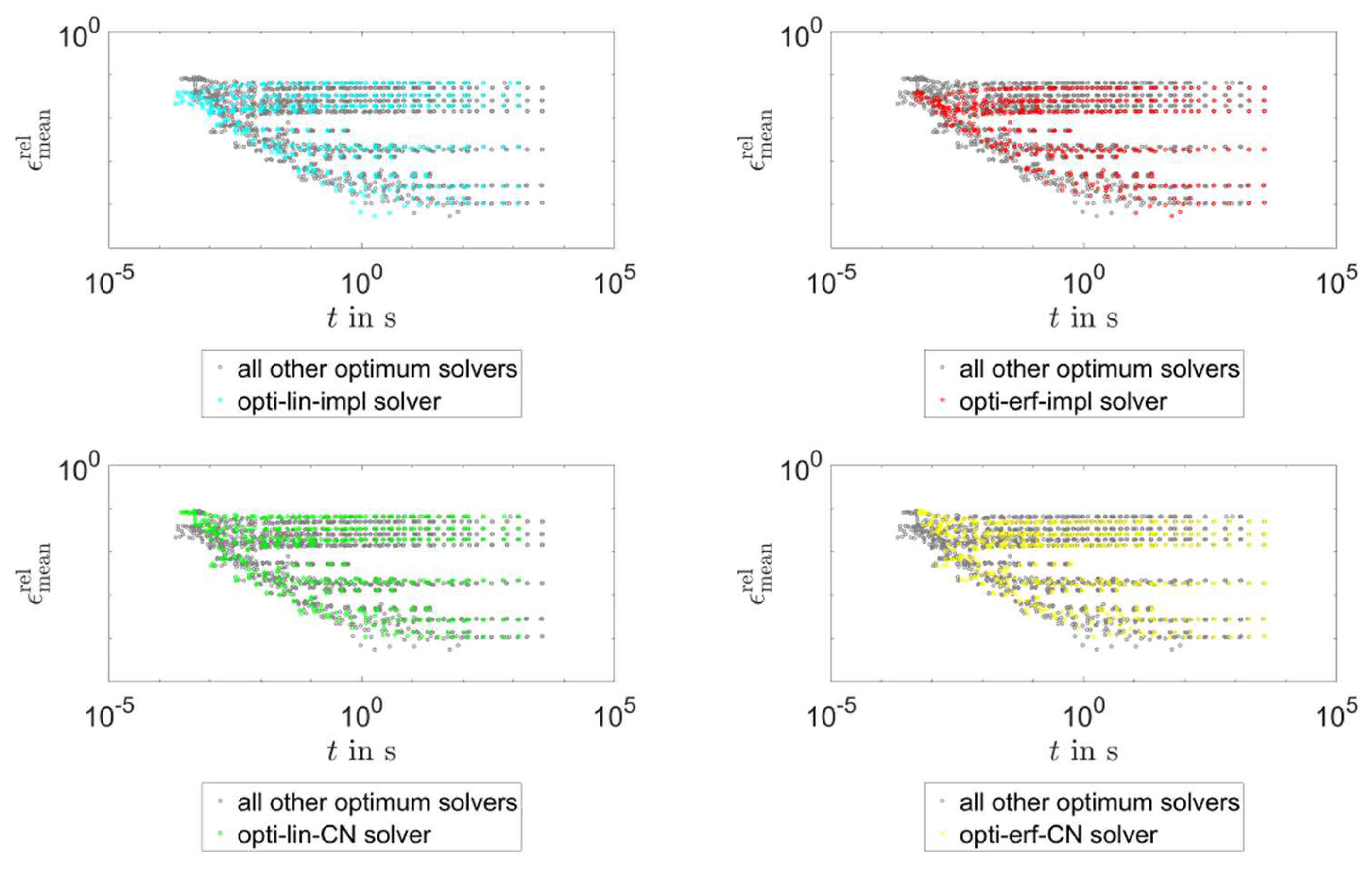
  • The optimum approach solvers needed fewer iterations if the c p , a p p function is linear, compared to the error function case; in addition, the temperature update is faster and easier to derive and program when a linear function is used. For the remaining solvers, relying on a c p , a p p , the implementation of an error function can increase the accuracy to some extent, but these methods are still, by far, not preferred over the optimum approach.
  • Does the use of higher-order methods for the time stepping give any benefit?
  • Using the MATLAB ODE solvers did not give any benefits, so it should only be an option when their use is mandatory due to the given simulation framework. Applying the Crank–Nicolson method instead of the implicit Euler method for the optimum approach solvers did not give significantly more accurate results for the same simulation time, and, in some cases, the implicit Euler method gave even more accurate results for the same simulation time. This underlines the fact that the accuracy is driven by a correct updating of the temperature/enthalpy relation and not by order of the discretization scheme of the transient term.
  • Which methods are appropriate when implementing the solid/liquid phase change in solvers with an automated time step control—like the ODE solvers in MATLAB? Moreover, how do they perform compared to the other solvers studied?
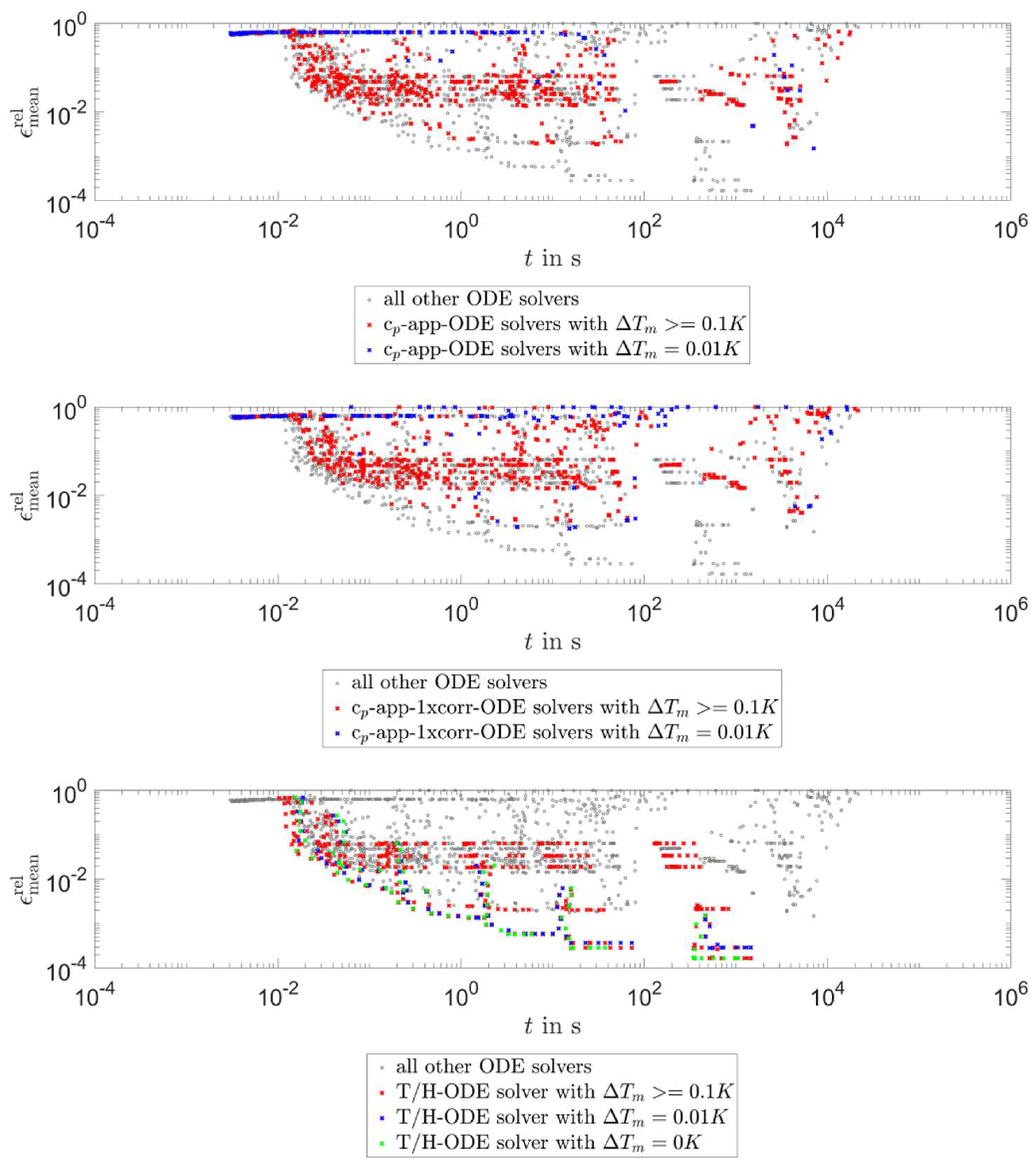
  • The best results for the MATLAB ODE solvers were achieved with a method (T/H-lin-ODE) developed from the basic explicit method, which uses the temperature field of the old-time step to calculate the new enthalpy field. This enthalpy field is then used to update the temperature field for the next time step. In terms of accuracy, this solver achieved results comparable to the optimum approach solvers. With the cp-app-ODE solvers, acceptable results were also achieved when the tolerance was set tight enough—the absolute value depends on the solver and the mesh—and the artificial melting temperature range width was chosen carefully. As a reference (based on the conditions applied in this work), values between 0.1 to 1 K can be used, which are not so large as to give errors due to the artificial melting temperature range itself and not so small as to over-jump the phase change region. Regarding the simulation time, a large discrepancy to the best solvers studied can be seen for all ODE solvers. For a given accuracy, the ODE solvers were up to two orders of magnitude slower.
  • Does linearizing the diffusion term instead of the transient term (i.e., the optimum approach) give any benefits?
Linearizing the diffusion term (lin-diff-lin-impl solver) gave much worse results than using the optimum approach.
Regarding the cp-app methods, it is already stated in the literature [5], that a correction/projection of the temperature (such as that introduced by Pham [20] and Comini [21]) can help to increase the stability. However, it did not outperform the optimum approach, mainly because it became unstable for large time steps. We found that the reason for this behavior lies in the updating of the temperature, which can give temperatures outside the boundaries defined by the neighboring cells (similar to an explicit method) when the cell jumps out of the phase change region. Unlike explicit methods, this behavior is damped to some extent by the next time steps and neighboring cells, leading to greater stability than with the explicit methods.

6. Conclusions

This study deals with different enthalpy methods for solving solid/liquid phase change problems. The methods were tested on a one-dimensional conduction-driven case for accuracy and numerical efficiency. Generally, the following conclusions can be drawn.
The projection/correction of the temperature/enthalpy relation is key, and it works best when this is performed iteratively. The so-called optimum approach [17,19] performed best in terms of accuracy and simulation time. Another solver that can be recommended is a basic explicit approach, which gives accurate results in an acceptable simulation time, too.
Therefore, the optimum approach is recommended if the simulation time is more important than the programming time. However, if the programming effort needs to be as low as possible, the basic explicit method is a very good alternative. It is easy to program, accurate, and has little numerical effort per time step—the only drawback is its limitations to t / t stab 1 .
Finally, the classical apparent heat capacity approaches (cp-app-lin-expl, cp-app-lin-impl, cp-app-erf-expl, cp-app-erf-impl) cannot be recommended, as they only gave acceptable results for a certain set of parameters, which includes time step sizes of t / t stab < 1 . As already stated in the literature [5], a correction/projection of the temperature (such as that introduced by Pham [20] and Comini [21]) helped but did not outperform the optimum approach, mainly because it became unstable for large time steps. A solver based on the idea of the optimum approach but with a linearization of the diffusion term instead of the transient term performed much worse than the optimum approach itself.
As for the influence of the varied parameters on the accuracy of the most accurate solvers (optimum approach solvers and the basic explicit solver), the minimum of the relative mean error was affected most by the number of nodes and the artificial melting temperature range. On the contrary, the influence of the time step was much smaller.
No matter the time step chosen, the minimum of the relative mean error was distinctly below 10−3.
Looking at the simulation time of the implicit methods with acceptable accuracy (optimum approach solvers and apparent heat capacity methods with one correction), the ranking of the varied parameters is different. Here, the width of the artificial melting temperature range had almost no influence, but the number of nodes (four orders of magnitude) and the time step size (two orders of magnitude) had a strong effect.
Comparing the implicit methods with the basic explicit method running with t / t stab = 1 revealed that, depending on the solver and the varied parameters, t / t stab needed ranged from 2.5–25 to achieve an equal simulation time for the implicit methods.
The use of higher-order methods for time discretization did not give any advantages except for solvers with an automated time step control. Here, the time step control allowed for obtaining acceptable results with uncorrected apparent heat capacity methods. However, it is important to note that solvers applying higher-order time discretization schemes, performing a projection between temperature and enthalpy, performed considerably more accurately than the aforementioned apparent heat capacity solvers without a projection. Moreover, the optimum approach with an implicit Euler time-stepping scheme was up to two orders of magnitude faster than the solvers with an automated time step control (ode15s solver from MATLAB).
Interestingly, the average number of iterations per time step was less than two for all optimum approach solvers, except for opti-erf-impl, which needed slightly more than two iterations per time step on average. For small time steps and large numbers of nodes, the number of iterations per time step was even almost equal to 1. This indicates that the optimum approach, as the one implemented here, is able to solve the equations correctly “at the first try” for many time steps, therefore, calling the need for a hybrid method [23] into question.
Future work will focus on the development of reduced-order models for the simulation of solid/liquid phase changes, whereas the results achieved in this study will serve as a benchmark.

Author Contributions

Conceptualization, A.K.-H. and G.D.; methodology, A.K.-H.; software, A.K.-H.; validation, A.K.-H. and G.D.; investigation, A.K.-H. and G.D.; writing—original draft preparation, A.K.-H.; writing—review and editing, G.D.; funding acquisition, A.K.-H. and G.D. All authors have read and agreed to the published version of the manuscript.

Funding

A.K.-H. is grateful for the financial support of the Deutsche Forschungsgemeinschaft (DFG, German Research Foundation) under Grant no 444616738/KO 6286/1-1.

Data Availability Statement

The data presented in this study are available on request from the corresponding author.

Acknowledgments

We would particularly like to thank Moritz Faden from the University of Bayreuth for the fruitful discussions.

Conflicts of Interest

The authors declare no conflict of interest.

Nomenclature

PropertyValueUnits
A ¯ c o e f coefficient matrix
c p heat capacity J k g · K
e r f c complementary error function
H enthalpy J
i time step count variable
l lengthm
L melting enthalpy J k g
n number of time steps or nodes
ODEordinary differential equation
q heat flux W m 2
R B boundary condition vector
t times
T temperatureK
t time step sizes
T temperature rangeK
x coordinate m
X phase front position m
α heat transfer coefficient W m 2 · K
ε error
λ thermal conductivity W m · K
ρ density k g m 3
subscripts
a m b ambient
a p p apparent
i time step count variable
i n i t Initial
j node count variable
k old iteration step
k + 1 new iteration step
l liquid
m melting
m e a n Mean
n e w New time step
o l d old time step
s solid
s t a b stability
t time step
t c test case
v a l validation case
x x-direction
superscripts
r e f reference
r e l relative
s i m simulation
T temperature
* preliminary

Appendix A

Figure A1. ε mean rel plotted over T m for simulations with cp-app solvers.
Energies 16 00449 g0a1
Figure A2. Ratio of simulations for all solvers with T m 0.1 that give ε mean rel < 1 % .
Energies 16 00449 g0a2
Figure A3. Required computing time over t / t stab for simulations of the opti-lin-impl solver compared to simulations of the T/H-lin-expl solver t / t stab = 1 .
Energies 16 00449 g0a3
Figure A4. Required computing time over t / t stab for simulations of the opti-lin-CN solver compared to simulations of the T/H-lin-expl solver t / t stab = 1 .
Energies 16 00449 g0a4
Figure A5. Required computing time over t / t stab for simulations of the opti-erf-impl solver compared to simulations of the T/H-lin-expl solver t / t stab = 1 .
Energies 16 00449 g0a5
Figure A6. Required computing time over t / t stab for simulations of the opti-erf-CN solver compared to simulations of the T/H-lin-expl solver t / t stab = 1 .
Energies 16 00449 g0a6
Figure A7. Required computing time over t / t stab for simulations of the cp-app-1xcorr-lin-impl solver compared to simulations of the T/H-lin-expl solver t / t stab = 1 .
Energies 16 00449 g0a7
Figure A8. Required computing time over t / t stab for simulations of the cp-app-1xcorr-erf-impl solver compared to simulations of the T/H-lin-expl solver t / t stab = 1 .
Energies 16 00449 g0a8

References

  1. Dutil, Y.; Rousse, D.R.; Salah, N.B.; Lassue, S.; Zalewski, L. A review on phase-change materials: Mathematical modeling and simulations. Renew. Sustain. Energy Rev. 2011, 15, 112–130. [Google Scholar] [CrossRef]
  2. Mackwood, A.P.; Crafer, R.C. Thermal modelling of laser welding and related processes: A literature review. Opt. Laser Technol. 2005, 37, 99–115. [Google Scholar] [CrossRef]
  3. Thomas, B.G.; Zhang, L. Mathematical modeling of fluid flow in continuous casting. ISIJ Int. 2001, 41, 1181–1193. [Google Scholar] [CrossRef]
  4. Pham, Q.T. Modelling heat and mass transfer in frozen foods: A review. Int. J. Refrig. 2006, 29, 876–888. [Google Scholar] [CrossRef]
  5. Voller, V.R. An overview of numerical methods for solving phase change problems. In Advances in Numerical Heat Transfer; Minkowycz, W.J., Sparrow, E.M., Eds.; Taylor & Francis: New York, NY, USA, 1997; pp. 341–380. [Google Scholar]
  6. Furzeland, R.M. A comparative study of numerical methods for moving boundary problems. IMA J. Appl. Math 1980, 26, 411–429. [Google Scholar] [CrossRef]
  7. Voller, V.R.; Swaminathan, C.R.; Thomas, B.G. Fixed grid techniques for phase change problems: A review. Int. J. Numer. Methods Eng. 1990, 30, 875–898. [Google Scholar] [CrossRef]
  8. Hu, H.; Argyropoulos, S.A. Mathematical modelling of solidification and melting: A review. Modell. Simul. Mater. Sci. Eng. 1996, 4, 371–396. [Google Scholar] [CrossRef] [Green Version]
  9. Basu, B.; Date, A.W. Numerical modelling of melting and solidification problems—A review. Sadhana 1988, 13, 169–213. [Google Scholar] [CrossRef]
  10. Bertrand, O.; Binet, B.; Combeau, H.; Couturier, S.; Delannoy, Y.; Gobin, D.; Lacroix, M.; Le Quéré, P.; Médale, M.; Mencinger, J.; et al. Melting driven by natural convection a comparison exercise: First results. Int. J. Therm. Sci. 1999, 38, 5–26. [Google Scholar] [CrossRef]
  11. Gobin, D.; Le Quéré, P. Melting from an isothermal vertical wall. Synthesis of a numerical comparison exercise. Comput. Assist. Mech. Eng. Sci. 1999, 7, 289–306. [Google Scholar]
  12. Pointner, H.; de Gracia, A.; Vogel, J.; Tay, N.; Liu, M.; Johnson, M.; Cabeza, L.F. Computational efficiency in numerical modeling of high temperature latent heat storage: Comparison of selected software tools based on experimental data. Appl. Energy 2016, 161, 337–348. [Google Scholar] [CrossRef]
  13. Tamma, K.K.; Namburu, R.R. Recent advances, trends and new perspectives via enthalpy-based finite element formulations for applications to solidification problems. Int. J. Numer. Methods Eng. 1990, 30, 803–820. [Google Scholar] [CrossRef]
  14. Mauder, T.; Charvat, P.; Stetina, J.; Klimes, L. Assessment of basic approaches to numerical modeling of phase change problems—Accuracy, efficiency, and parallel decomposition. J. Heat Transf. 2017, 139, 084502. [Google Scholar] [CrossRef]
  15. König-Haagen, A.; Franquet, E.; Faden, M.; Brüggemann, D. Influence of the convective energy formulation for melting problems with enthalpy methods. Int. J. Therm. Sci. 2020, 158, 106477. [Google Scholar] [CrossRef]
  16. König-Haagen, A.; Franquet, E.; Faden, M.; Brüggemann, D. A study on the numerical performances of diffuse interface methods for simulation of melting and their practical consequences. Energies 2021, 14, 354. [Google Scholar] [CrossRef]
  17. Swaminathan, C.R.; Voller, V.R. On the enthalpy method. Int. J. Numer. Methods Heat Fluid Flow 1993, 3, 233–244. [Google Scholar] [CrossRef]
  18. Voller, V.R.; Swaminathan, C.R. General source-based method for solidification phase change. Numer. Heat Transf. Part B 1991, 19, 175–189. [Google Scholar] [CrossRef]
  19. Swaminathan, C.R.; Voller, V.R. A general enthalpy method for modeling solidification processes. Metall. Trans. B 1992, 23, 651–664. [Google Scholar] [CrossRef]
  20. Pham, Q.T. A fast, unconditionally stable finite-difference scheme for heat conduction with phase change. Int. J. Heat Mass Transf. 1985, 28, 2079–2084. [Google Scholar] [CrossRef]
  21. Comini, G.; Giudice, S.D.; Saro, O. A conservative algorithm for multidimensional conduction phase change. Int. J. Numer. Methods Eng. 1990, 30, 697–709. [Google Scholar] [CrossRef]
  22. Pham, Q.T. Comparison of general-purpose finite-element methods for the Stefan problem. Numer. Heat Transf. Part B 1995, 27, 417–435. [Google Scholar] [CrossRef]
  23. Al-Saadi, S.N.; Zhai, Z. Systematic evaluation of mathematical methods and numerical schemes for modeling PCM-enhanced building enclosure. Energy Build. 2015, 92, 374–388. [Google Scholar] [CrossRef]
  24. Kuznik, F.; Johannes, K.; Franquet, E.; Zalewski, L.; Gibout, S.; Tittelein, P.; Dumas, J.-P.; David, D.; Bédécarrats, J.-P.; Lassue, S. Impact of the enthalpy function on the simulation of a building with phase change material wall. Energy Build. 2016, 126, 220–229. [Google Scholar] [CrossRef]
  25. Dal Magro, F.; Jimenez-Arreola, M.; Romagnoli, A. Improving energy recovery efficiency by retrofitting a PCM-based technology to an ORC system operating under thermal power fluctuations. Appl. Energy 2017, 208, 972–985. [Google Scholar] [CrossRef]
  26. Griesbach, M.; König-Haagen, A.; Brüggemann, D. Numerical analysis of a combined heat pump ice energy storage system without solar Benefit—Analytical validation and comparison with long term experimental data over one year. Appl. Therm. Eng. 2022, 213, 118696. [Google Scholar] [CrossRef]
  27. Faden, M.; König-Haagen, A.; Höhlein, S.; Brüggemann, D. An implicit algorithm for melting and settling of phase change material inside macrocapsules. Int. J. Heat Mass Transf. 2018, 117, 757–767. [Google Scholar] [CrossRef]
  28. Kozak, Y.; Ziskind, G. Novel enthalpy method for modeling of PCM melting accompanied by sinking of the solid phase. Int. J. Heat Mass Transf. 2017, 112, 568–586. [Google Scholar] [CrossRef]
  29. Hummel, D.; Beer, S.; Hornung, A. A conjugate heat transfer model for unconstrained melting of macroencapsulated phase change materials subjected to external convection. Int. J. Heat Mass Transf. 2020, 149, 119205. [Google Scholar] [CrossRef]
  30. Kasibhatla, R.R.; Brüggemann, D. Coupled conjugate heat transfer model for melting of PCM in cylindrical capsules. Appl. Therm. Eng. 2021, 184, 116301. [Google Scholar] [CrossRef]
  31. Stefan, J. Uber einige probleme der theorie der warmeletung. Sitzungsber. Akad. Wiss. Wien Math.-Naturwiss. 1889, 98, 473–484. [Google Scholar]
  32. Lamé, G.; Clapeyron, B.P. Mémoire sur la solidification par refroidissement d’un globe liquide. Ann. Chim. Phys. 1831, 47, 250–256. [Google Scholar]
  33. Tarzia, D. An explicit solution for a two-phase unidimensional Stefan problem with a convective boundary condition at the fixed face. MAT-Ser. A 2004, 8, 21–27. [Google Scholar]
  34. Ma, Z.W.; Zhang, P. Modeling the heat transfer characteristics of flow melting of phase change material slurries in the circular tubes. Int. J. Heat Mass Transf. 2013, 64, 874–881. [Google Scholar] [CrossRef]
  35. Schiesser, W.E.; Griffiths, G.W. A Compendium of Partial Differential Equation Models: Method of Lines Analysis with Matlab; Cambridge University Press: New York, NY, USA, 2009. [Google Scholar]
Figure 1. Classification of the enthalpy method with typical solvers as examples.
Energies 16 00449 g001
Figure 2. Sketch of the physical problem.
Energies 16 00449 g002
Figure 3. Examples of c p , a p p and H plotted over T for different T m .
Energies 16 00449 g003
Figure 4. ε mean of the numerical reference model (T/H-lin-expl) compared to the exact analytical solution plotted over the number of nodes.
Energies 16 00449 g004
Figure 5. Required computing time and ε mean rel for all simulations.
Energies 16 00449 g005
Figure 6. Required computing time and ε mean rel for all simulations performed with the optimum approach solvers.
Energies 16 00449 g006
Figure 7. Required computing time and ε mean rel for simulations performed with ODE solvers.
Energies 16 00449 g007
Figure 8. ε mean rel plotted over T m for simulations of the T/H-lin-expl solver and the optimum approach solvers.
Energies 16 00449 g008
Figure 9. ε mean rel plotted over the number of nodes of the T/H-lin-expl solver and the optimum approach solvers.
Energies 16 00449 g009
Figure 10. ε mean rel plotted over t / t stab for simulations of the T/H-lin-expl solver and the optimum approach solvers.
Energies 16 00449 g010
Figure 11. Number of iterations per time step over T m for simulations with the optimum solvers.
Energies 16 00449 g011
Figure 12. Number of iterations per time step over the number of nodes for simulations with the optimum approach solvers.
Energies 16 00449 g012
Figure 13. Number of iterations per time step over t / t stab for simulations with the optimum solvers.
Energies 16 00449 g013
Table 1. Material properties, initial and boundary conditions for the test case and the validation.
PropertyValueUnits
T i n i t 52°C
T a m b 32°C
α 1000 W m 2 · K
T m 42°C
c p 2000 J k g · K
L 200,000 J k g
ρ 1000 k g m 3
λ 1 W m · K
l t c 0.1 m
l v a l 1 m
Table 2. Overview of the solvers and their identifiers.
IdentifierCorrecting ApproachSlope of the T/H RelationTime Stepping
T/H-lin-explcorrected *linearfixed-step explicit
T/H-lin-ODEcorrected *linearvariable step ode15s
cp-app-lin-expluncorrectedlinearfixed-step explicit
cp-app-lin-impluncorrectedlinearfixed-step implicit
cp-app-erf-expluncorrectederror functionfixed-step explicit
cp-app-erf-impluncorrectederror functionfixed-step implicit
cp-app-lin-ODEuncorrectedlinearvariable step ode15s
cp-app-erf-ODEuncorrectederror functionvariable step ode15s
cp-app-1xcorr-lin-explone correctionlinearfixed-step explicit
cp-app-1xcorr-lin-implone correctionlinearfixed-step implicit
cp-app-1xcorr-erf-explone correctionerror functionfixed-step explicit
cp-app-1xcorr-erf-implone correctionerror functionfixed-step implicit
cp-app-1xcorr-lin-ODEone correctionlinearvariable step ode15s
cp-app-1xcorr-erf-ODEone correctionerror functionvariable step ode15s
opti-lin-implIterative correctionlinearfixed-step implicit
opti-erf-implIterative correctionerror functionfixed-step implicit
opti-lin-CNIterative correctionlinearfixed-step Crank–Nicolson
opti-erf-CNIterative correctionerror functionfixed-step Crank–Nicolson
lin-diff-lin-implIterative correctionlinearfixed-step implicit
* The temperature is corrected at the end of the time step but only used in the next time step.
Table 3. Overview of the parameter variations.
Solvers t Variation [ t t s t a b ] T m Variation [K]Rel. Tolerance [-]Mesh [Number of Nodes]
opti-lin-impl
opti-erf-impl
opti-lin-CN
opti-erf-CN
lin-diff-lin-impl
0.1, 0.2, 0.5, 1, 2, 4, 9, 18, 36, 72, 144, 2160, 0.01, 0.1, 1, 2, 5-10, 20, 50, 100, 200, 500
cp-app-lin-impl
cp-app-erf-impl
cp-app-1xcorr-lin-impl
cp-app-1xcorr-erf-impl
0.1, 0.2, 0.5, 1, 2, 4, 9, 18, 36, 72, 144, 2160.01, 0.1, 1, 2, 5-10, 20, 50, 100, 200, 500
T/H-lin-expl0.1, 0.2, 0.5, 10, 0.01, 0.1, 1, 2, 5-10, 20, 50, 100, 200, 500
cp-app-lin-expl
cp-app-erf-expl
cp-app-1xcorr-lin-expl
cp-app-1xcorr-erf-expl
0.1, 0.2, 0.5, 10.01, 0.1, 1, 2, 5-10, 20, 50, 100, 200, 500
T/H-lin-ODE-0, 0.01, 0.1, 1, 2, 51 × 10−9, 1 × 10⁻⁸,
1 × 10⁻⁷, 1 × 10⁻⁶,
1 × 10⁻⁵, 1 × 10⁻⁴,
2 × 10⁻⁴, 5 × 10⁻⁴,
1 × 10⁻³, 2 × 10⁻³,
5 × 10⁻³, 1 × 10⁻²
10, 20, 50, 100, 200, 500
cp-app-lin-ODE
cp-app-erf-ODE
cp-app-1xcorr-lin-ODE
cp-app-1xcorr-erf-ODE
-0.01, 0.1, 1, 2, 51 × 10−9, 1 × 10⁻⁸,
1 × 10⁻⁷, 1 × 10⁻⁶,
1 × 10⁻⁵, 1 × 10⁻⁴,
2 × 10⁻⁴, 5 × 10⁻⁴,
1 × 10⁻³, 2 × 10⁻³,
5 × 10⁻³, 1 × 10⁻²
10, 20, 50, 100, 200, 500
Table 4. List of t / t stab values needed to be faster with implicit solvers than the basic explicit solver T/H-lin-expl.
Solver t / t stab Figures
opti-lin-impl≈3–7Figure A3 in the Appendix A
opti-lin-CN≈3–8Figure A4 in the Appendix A
opti-erf-impl≈3.5–20Figure A5 in the Appendix A
opti-erf-CN≈4–20Figure A6 in the Appendix A
cp-app-1xcorr-lin-impl≈2.5–15Figure A7 in the Appendix A
cp-app-1xcorr-erf-impl≈3.5–25Figure A8 in the Appendix A
Disclaimer/Publisher’s Note: The statements, opinions and data contained in all publications are solely those of the individual author(s) and contributor(s) and not of MDPI and/or the editor(s). MDPI and/or the editor(s) disclaim responsibility for any injury to people or property resulting from any ideas, methods, instructions or products referred to in the content.

