Abstract
Electrical utilities and system operators (SOs) are constantly looking for solutions to problems in the management and control of the power network. For this purpose, SOs are exploring new research fields, which might bring contributions to the power system environment. A clear example is the field of computer science, within which artificial intelligence (AI) has been developed and is being applied to many fields. In power systems, AI could support the fault prediction of cable joints. Despite the availability of many legacy methods described in the literature, fault prediction is still critical, and it needs new solutions. For this purpose, in this paper, the authors made a further step in the evaluation of machine learning methods (ML) for cable joint health assessment. Six ML algorithms have been compared and assessed on a consolidated test scenario. It simulates a distributed measurement system which collects measurements from medium-voltage (MV) cable joints. Typical metrics have been applied to compare the performance of the algorithms. The analysis is then completed considering the actual in-field conditions and the SOs’ requirements. The results demonstrate: (i) the pros and cons of each algorithm; (ii) the best-performing algorithm; (iii) the possible benefits from the implementation of ML algorithms.
1. Introduction
The recent social, economic, and environmental changes are affecting and challenging the electric grid. Countries and system operators (SOs) need to enhance and adapt how the grid is managed and controlled.
For example, there is an urgent need to find alternatives to fossil fuels for energy production. However, it is well known that a significant percentage of renewables in the production mix affect the healthy grid [1,2,3]. Therefore, researchers are: (i) creating new and adapting models [4] to include different renewable-based scenarios; (ii) analyzing the impact on the energy markets and the price level [5,6]; (iii) mitigating the effect of renewables on the voltage stability [7]; etc.
At the same time, transport electrification is demanding grid flexibility to support the introduction of new assets. Electric vehicles are not only changing the paradigms of transportation and people’s mobility, but they are also affecting the other assets’ performance and aging [8], the generation/load balance [9,10], and the energy costs [11].
The changes to the electric grid need to be addressed by SOs. For example, an innovative generation of instrument transformers (ITs), the low-power ITs (LPITs), has been recently introduced into the grid. They are standardized by the IEC 61869 series, in which IEC 61869-10 and -11 describe the current and voltage (LPCT and LPVT) versions of LPITs, respectively [12,13]. LPITs are gradually replacing legacy ITs because they are smaller, lighter, and cheaper and have a wider bandwidth compared to them. Therefore, studies relevant to their characterization [14], aging [15], use for protective purposes [16], and design [17] are populating the literature.
Another solution that SOs are exploring comes from computer science. Artificial intelligence (AI) is considered one of the key tools that will help in dealing with incoming challenges.
Its advent is bringing enhancements and benefits to a variety of fields. AI is applied to medicine [18], education [19], economics [20], and even psychology [21]. Therefore, it is very probable that power systems will benefit from its application as well. Some examples are available in the literature. AI is used (i) in [22] for optimal reactive power management; (ii) in [23] for the integration with MPPT techniques; (iii) in [24] to determine which customers are connected to the grid; and (iv) in [25] to be applied to a variety of power electronic fields.
In this paper, AI is applied in support of the detection of faults in medium-voltage (MV) distribution network cable joints. The failure of a cable joint is the main cause of faults in MV networks, and it results in huge economic losses in high-voltage (HV) ones. Consequently, many works in the literature deal with the topic. A thermal model to detect defects is described in [26], while [27] suggests the implementation of space charge measurements. In [28], instead, partial discharge (PD) measurements are performed on HVDC cables.
The idea of applying AI to the fault prediction of cable joints has been introduced in [29]. Considering the promising results, this paper focuses on algorithm selection and design. Six ML algorithms have been selected and compared in a realistic cable joint scenario. Emphasis is given to the characteristics of a distributed measurement system capable of measuring the required quantities. Furthermore, it is clarified that, to date, there are no clear thresholds that indicate the imminent fault of a cable joint. Hence, ML-based methods, such as the legacy ones, can only support the difficult decision to be made by SOs. Overall, there are two main goals. One is to find the pros and cons of the selected algorithms, highlighting the best-performing one/s. The second is the analysis of the benefits of the ML algorithms applied to the fault prediction of cable joints.
The remainder of the paper is structured as follows. Section 2 describes some basic concepts of artificial intelligence and computer science used in the following chapters. In Section 3, the reader is introduced to cable joints and their characteristics. The case study considered in this work is detailed in Section 4. Afterwards, Section 5 and Section 6 contain the tests and results performed and obtained according to the case study. Finally, Section 7 summarizes the achievements and concludes the work.
2. Artificial Intelligence Background
2.1. Overview
AI is a branch of computer science that studies the design of hardware systems and software programs to simulate processes of human intelligence. The main addressed tasks are reasoning, learning, adaptation, planning, and visual or space-time perception.
Depending on the development principle of AI technologies, this discipline is divided into strong and weak AI. The strong AI is based on the idea that machines can develop a self and autonomous conscience, while weak AI believes that machines can only carry out required processes without a real awareness of their activities [30].
In general, AI systems work by analyzing a large quantity of data to find patterns and correlations and use them to obtain forecasts or assessments of future statements.
Machine learning (ML) is a field of AI based on the ability of systems to automatically learn from data. This skill is due to the ability of ML algorithms to modify their processes in order to adapt them to the data, applying mathematical and computational strategies without using predetermined equations or models. Therefore, algorithms can increase their efficiency after completing a task, and their explicit programming is not needed.
The recent and sudden development of ML is fundamentally due to two enabling aspects: the availability of large amounts of data and the wide computing capacity that is provided by the tools available today.
Deep learning is one of the main ML techniques and a subfield based on Artificial Neural Networks (ANNs). ANNs are structures made of elementary units (called neurons or nodes) organized in different layers that are specifically interconnected. These systems have the aim of simulating the human brain architecture to automate parts of the data processing, eliminating some of the actions required by standard ML algorithms. This procedure of automatic optimization is achievable by the ability of ANNs to modify the values of their parameters in function of the processed data.
In summary, AI is a computer science field which simulates human intelligence processes. One of the ways to achieve this is by using ML techniques. These are divided into supervised, unsupervised, and reinforcement learning algorithms, according to their method of learning from data [31].
Supervised learning uses labeled input data, i.e., input–output pairs, to understand the existing relationship and use it to provide outputs for unknown inputs. These algorithms can be used in classification or regression problems: in the first case, the output values are discrete, while in the second case, the values are continuous. Classification problems can also be divided into binary or multi-class tasks, depending on the number of values that the single output can take.
On the other hand, unsupervised learning uses unlabeled or unstructured data to find the existing structure or pattern. An example of this learning method is clustering, which provides groups of homogeneous elements starting from a heterogeneous set of data.
Considering supervised learning algorithms, their implementation involves two phases: the first is the learning stage, in which part of the dataset (training/learning set) is provided to the algorithm and used to find correlations and modeling. The second phase is the testing stage, in which the remaining part of the dataset (test set) is used to compare the outputs predicted by the algorithm and the correct ones.
2.2. Algorithms
This paper deals with binary classification problems. Some of the most popular algorithms are Logistic Regression (LR), Support Vector Machine (SVM), K-Nearest Neighbors (KNN), Decision Tree (DT), Random Forest (RF), and ANN. Generally, each algorithm has its predisposition to specific application fields, different types of data and structures, and the tendency to better perform increasing or reducing the learning samples.
The LR algorithm is a type of statistical model based on the use of the logistic (sigmoid) function, which binds a generic input value to an output value between 0 and 1. The algorithm works by finding a weight value used to calculate the input of the sigmoid function, starting from the real input data [32].
The SVM algorithm is based on the construction of an optimal hyperplane which correctly classifies the data [33]. In the binary classification case, this hyperplane is a straight line which divides the two-dimensional plane into two parts, corresponding to the two output classes. The optimal hyperplane is the one that maximizes the distance between the closest elements (support vectors) of the two different classes.
The KNN algorithm classifies data due to their similarity to and/or distance from the previous ones, supposing that close data have similar outputs [34]. This algorithm works by searching, in the training set, for the most similar K instances (the neighbors) and finding the output value with the highest frequency among these K elements. Such an output is the one given to the new input data. The calculation of the distance between the points can be carried out in several ways, e.g., the Euclidean one, the distance of Manhattan, Minkowski, or Hamming, etc.
A decision tree is a structure made of nodes and leaves. Nodes represent the points in which the data are separated, and the leaves represent the intermediate or final results of such separation. Each node is a conditional function which verifies the existence of a property for the evaluated data. The DT algorithm is based on this structure, and the working process consists of a sequence of tests, starting from the top node and working downwards [32]. The goal of the algorithm is to find the optimal split function that is capable of dividing data into two groups which are, internally, the most homogeneous possible (and, externally, the most heterogeneous possible) in order to minimize the difficulty of classification.
The RF algorithm is obtained by aggregating more decision trees which are fed with different training sets, randomly obtained from the original one [35]. The result is then calculated by choosing the most frequent one among all the produced outputs by the different Decision Tree algorithms that make up the forest.
As for ANNs, there are several types and variants of these algorithms [36]. In general, each elementary unit is characterized by an activation function, which represents the relationship between the input and the output signals of the neuron, and by a bias value, which realizes a shift in the input value of the neuron. All neurons are organized in layers and linked together in specific ways. Each connection is characterized by a weight value. An ANN aims to model the relation between input and output data by varying the values of its weights during the training stage through appropriate learning techniques.
3. The Cable Joint
This section provides an overview of cable joints. First, in Section 3.1, they are introduced, and their role in the distribution network is explained. Then, Section 3.2 details the types of cable joints, specifying their typical design. In Section 3.3, instead, the modes of fault are introduced. Finally, Section 3.4 contains an overview of the main quantities/parameters measured/computed to diagnosticate faults in cable joints.
3.1. Introduction
Power cables are one of the two possible ways to extend the power network. They are also the preferred solution in urban areas, where it is not always possible to build overhead lines. To add new power cables, cable joints are used. They allow for overcoming the limits fixed by the production process of power cable coils in terms of diameter, weight, and transport possibilities. Cable joints are often installed every 500–800 m; consequently, their number is considerable.
There are mainly two drawbacks resulting from the use of cable joints: a high failure rate and the difficulty of replacement [37,38]. The former problem is due to the different types of stress that affect cable joints, such as mechanical, thermal, electrical, and environmental stress. Furthermore, they are typically buried several meters deep in the ground. One of the current technological challenges is to increase their reliability in order to reduce the number of faults in the distribution network. As a matter of fact, cable joints are the main cause of faults in MV lines, and the most frequent failure mode is due to the breakdown of the electrical insulation.
By comparing the average life of a power cable (30–40 years) with the one of a cable joint (7–8 years), it can be concluded that they significantly affect the performance of the overall network [37,38]. Furthermore, installation methods, laying conditions, and characteristics of the surrounding environment (type of soil, humidity, temperature, etc.) can drastically speed up the cable joint aging.
In the event of the failure of a cable joint, it is necessary to isolate the surrounding portion of the network and proceed with the replacement. This process is costly and results in a disservice to the users and penalties to be paid by the SO. It is then crucial to investigate the fault causes of cable joints. The results would improve the reliability of the grid and the savings of SOs.
3.2. Description
A cable joint is an electrical asset that joins two portions of the cable. The cable joint ensures electrical continuity at the connection point, insulation continuity, mechanical resistance, and physical protection from the external environment.
Depending on the function, the type of connection, the type of cable, and the construction materials, different types of joints are identified. As for the design, it is typically based on the current and voltage values to which they are subjected and on the conditions of the environment in which they are installed.
There are two macro-categories of joints: heat-shrinkable and cold-shrinkable cable joints. The heat-shrinkable joints are shown in Figure 1 and are typically made of a polymeric material (rubber-plastic) that shrinks once heated up. In this way, once installed, the heat source makes the cable joint adhere to the cable.
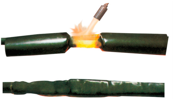
Figure 1.
An example of a heat-shrinkable cable joint during its installation.
The cold-shrinkable joint is shown in Figure 2. They are typically made of silicone rubber, which is expanded onto a rigid spiral core. Once installed on the cable, the spiral is pulled out, and the joint gradually adheres to the cable.
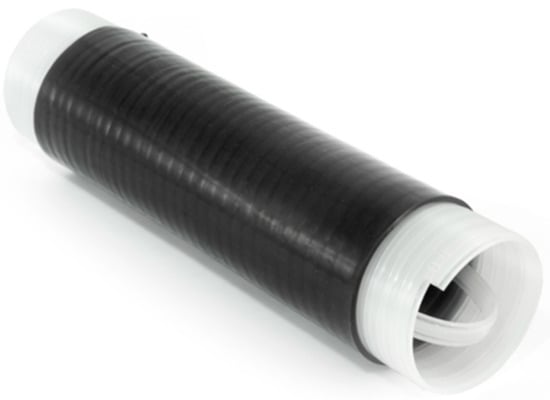
Figure 2.
An example of a cold-shrinkable cable joint before its installation.
As far as the constituent material is concerned, silicone rubber has excellent insulating properties and a high elasticity, a characteristic that is absent in the polymer constituting the heat-shrinking joints. Furthermore, the two types of joints differ in two additional aspects. First, the cold-shrinkable joints are prefabricated through high-pressure and high-temperature processes. Therefore, during the installation, removing the spiral is the only action required (limiting the risks). On the other hand, the heat-shrinkable joints installation process is more prone to risks due to the need for a heat source.
Second, according to their design, cold-shrinkable joints adapt perfectly to the cable, limiting the formation of voids or water leakage. As for the heat-shrinkable ones, they have limited elasticity, resulting in less resistance to mechanical stress and thermal cycles. Overall, cold-shrinkable cable joints are the most used type of joint in distribution networks.
Their generic structure is depicted in Figure 3. From it, four layers are identified. Starting from the outermost one, these are: cold-shrinkable insulation, metal shield, silicone rubber insulating layer, semiconductive layers, and metal connector.
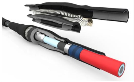
Figure 3.
The internal structure of a cold-shrinkable cable joint.
As mentioned above, cold-shrinkable insulation guarantees electrical insulation and protection from mechanical stress.
The metal screen consists of thin conducting and intertwined wires that share the earth’s potential between the two portions of the cable. The metal screen also limits disturbances from the outside.
The silicone rubber insulating layer is preceded and followed by layers of semiconductive material to uniformize the electric field.
The metal connector creates the mechanical connection between the two conductors and contributes to the mechanical protection of the latter.
3.3. Modes of Fault
The most frequent failure mode for these accessories is the failure of the electrical insulation, which is typically identified as the only failure mode following the wear and/or aging of the insulation itself. However, this degradation is a very complex phenomenon which may result from various causes and, in turn, may have various consequences.
Other failure modes are (i) the breakdown of the main insulation or the cable insulation, (ii) thermal breakdown in the dielectric and failure in the connection point of the conductors, and (iii) failure in the sheath and at the cable–joint interface. The main causes of these failures are the establishment of partial discharges and the development of electrical or water treeing. These phenomena are interconnected and are typically due to overvoltage, overheating, excessive current, the presence of defects or gaps in the insulation, stresses due to thermal cycling, mechanical stress, the ingress of water or humidity due to damage to the cable sheath, thermal runaway, the relaxation or mechanical failure of components, the breakage or short-circuiting of electrical conductors, and direct damage [37,38,39]. In addition, a failure can be due to aging, poor manufacturing, the presence of manufacturing defects, mechanical damage due to the poor mechanical strength of the external coating, improper laying, or incorrect installation. Table 1 summarizes the different failure modes and some of their causes.

Table 1.
Typical failure modes and causes of failure.
3.4. Measured Parameters
To prevent the failure of cable joints, various parameters can be monitored. Some are environmental factors, such as temperature, pressure, and humidity; others are electrical, such as current, voltage, electric field, partial discharges, and tangent delta.
Partial discharges are measured and classified to distinguish the faults [40], locate their source, identify the fault point [41], or estimate the aging state of the joint insulation [42,43]. Current measurements are exploited to detect a failure or defect in [39]. Pressure and temperature [44] or electric field [45] measurements allow for evaluating the quality of the dielectric by calculating its tan delta [46,47].
Another important aspect to consider in the evaluation of these parameters is that they are all strongly interconnected. In the literature, many studies investigate the relationship between electrical and non-electrical quantities. The goal that unites these studies is to correlate the measured quantities to the processes that lead to a breakdown (hence, preventing them). In [48], the relationship between temperature and tan delta is investigated, and it is observed how the latter quantity increases as the temperature decreases.
The correlation between tan delta and pressure is also studied. In [49], three different joints are tested to find the correlation between these two quantities.
Finally, an interesting correlation has been found between pressure and temperature. In [50,51], through the stress of thermal cycle joints, it was found that an increase in temperature leads to an increase in pressure. In [52], a correlation was demonstrated between the failures and the ambient temperature.
As already expressed above, all the parameters are strongly interconnected, and their relationships are extremely complex. A thorough understanding of these aspects is essential to assessing the integrity of the joints and their constituent parts. In addition, the analysis of the temporal evolution of the quantities of interest is crucial for the diagnosis and prevention of cable joint faults.
4. Case Study
This section describes the case study in which the tests described in Section 5 are performed. First, Section 4.1 lists the selected algorithms. Second, Section 4.2 introduces the quantities related to the cable joint monitoring. Third, Section 4.3 provides the set of metrics selected for the evaluation of the performed tests.
4.1. Considered Algorithms
A set of six algorithms has been selected for the sake of comparison and evaluation. The set consists of LR, SVM, KNN, DT, RF, and ANN. They are the typical algorithms implemented in the literature for binary classification tasks. For the implementation of the selected algorithms, the Scikit Learn library [53] in Python language has been used. No tuning has been applied to the algorithms. As described in Section 2, each algorithm has advantages and disadvantages depending on its application. However, they are all suitable for being assessed in the cable joint case study. As a matter of fact, no common or standard practice is available for the application of AI to power systems.
4.2. Considered Quantities
4.2.1. Overview
This section is critical to understanding the entire case study. Let us start with the concept that the cable joint health diagnosis is made by assessing measures. Such measures, which can be electrical or environmental quantities, are collected by distributed measurement systems. They are typically installed on the cable joint or its premises. Therefore, each measurement is representative of a local situation (in all kinds of networks). Note that a distributed measurement system may collect one or more quantities, and there is no regulation regarding the number nor regarding the way it is carried out. This case study, though, simulates the collection of the quantities of interest from several distributed measurement systems. The aim is to simulate an SO who periodically receives the measurement from the field.
There are four considered quantities: temperature, tangent delta, current, and the age of the cable joint. The temperature on the surface of the cable joint is precious information. The tangent delta is considered one of the most reliable electrical parameters that are to be monitored. The current is directly correlated with the temperature and the loading capacity of the cable. Finally, even if it is not obtained from the measurement, the age of the cable joint is certainly a diagnostic input.
Regarding the number of considered quantities, three (directly obtained from the joint) is a realistic number for two main reasons. First, the installation of measurement systems on cable joints is a complex and expensive operation; therefore, they are seldom deployed to collect only one quantity. Second, for each measured quantity, the complexity of the distributed measurement system sharply increases. Consequently, very few applications involving more than three/four quantities can be found.
4.2.2. Testing Details
Considering that the quantities of interest are simulated, their range of variation should be defined and motivated. For this purpose, Table 2 lists, for each quantity, the relevant range of variation.
Table 2.
Variation ranges of the quantities of interest.
The temperature and age limits are defined according to the commercial cables and cable joints datasheets. Of course, the temperature may vary within different limits. However, the idea is to define one illustrative scenario, which can be customized for other applications, to present the proposed approach. The tangent delta limits have been fixed, including insulating materials with different performances. Lastly, the current limits reflect the actual conditions of an in-field MV cable. Its operation may vary from no load condition (0 A) to the cable ampacity. Therefore, a maximum realistic value of 300 A is considered.
Once the limits are fixed, the last choice is the probability distribution of the samples to be generated during the tests. In this paper, the uniform and normal distributions have been selected. To increase the comprehension, a flowchart of the algorithm is depicted in Figure 4.
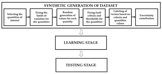
Figure 4.
Flowchart of the algorithm.
4.3. Metrics
The ML algorithm outputs are a set of predictions with a probabilistic nature, which distinguish positive from negative results. Therefore, it is important to quantify the performance of such algorithms to obtain the desired level of accuracy. To this purpose, several metrics can be used to quantify the accuracy of a model and its actual performance. For the considered case study, the metrics of accuracy, precision, and recall have been selected.
4.3.1. Accuracy
Accuracy is the ratio between the number of correct predictions and the total number of predictions made by the algorithm or, equally, the number of samples in the test set. Thus, it is a number between 0 and 1 and can also be expressed as a percentage.
This metric is the most adopted, as it provides a clear indication of the model performance. However, this metric does not always reflect the effective efficiency [31]. It does not consider the actual values of the model results but only how many of these are correct.
4.3.2. Confusion Matrix
The confusion matrix, unlike accuracy, considers both the predicted and the actual values, providing an overall picture. Four categories of results are defined: True Positive (TP), True Negative (TN), False Positive (FP), and False Negative (FN). A result is TP (or TN) if it is labeled as positive (or negative) in the test set and comes correctly predicted by the algorithm. Instead, an FP (or FN) is a positive (or negative) labeled outcome that is incorrectly predicted by the algorithm [31].
A generic confusion matrix can be represented, as shown in Figure 5. The colors in the figure help to distinguish between the correct and incorrect predictions.
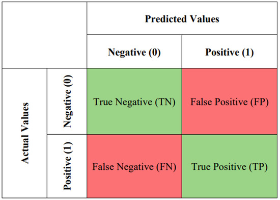
Figure 5.
An example of a confusion matrix.
The total correct predictions are the sum of TN and TP, while the total incorrect ones are the sum of FN and FP. Thus, the accuracy introduced in Section 4.3.1 can be calculated as:
4.3.3. Precision
Precision is the ratio between the correctly predicted positive values and the overall number of positive predictions [54]. Thus, while accuracy expresses the proximity of the model to the actual results, precision quantifies the consistency of the results, ignoring the achievement of the goal.
4.3.4. Recall
Recall is the ratio between the number of correctly predicted positive values and the total number of actual positive results in the test set [54].
5. Description of the Tests
Each test in what follows is designed to stress a particular aspect that may become critical in the final choice of the algorithm.
5.1. Number of Samples for the Learning Stage
The decision on the number of samples to be used in the learning stage is always critical. However, once made, the algorithms work most efficiently. Therefore, the first test aims to find, for each algorithm, the minimum number of samples that maximizes the algorithm’s accuracy. Of course, there is no closed formula to assess the goodness of the results. However, the choice is made by evaluating the results with a realistic perspective.
For this purpose, the six algorithms are tested using 100, 200, 500, 1000, 2000, 5000, and 10,000 samples for the learning stage and 100,000 for the testing stage.
5.2. Repeatability
As in the case of measurements, the repeatability of AI algorithms must be verified. Therefore, the algorithms were run 500 times with a specific set of conditions: 1000 learning samples, 100,000 testing samples, and a uniform distribution.
5.3. Data Distribution
The guide to the expression of uncertainty in measurements (GUM) [55] states that, in a case of a lack of information, one may assume a uniform distribution for the data (worst case). This is the reason for choosing it as one of the tested distributions. However, in some cases, one may have further information (or experience) to adopt other distributions. Therefore, starting from the conclusion of [29], for each algorithm, the results obtained with the normal distributions have been compared with those obtained from the uniform one. The test involved all the learning samples used for the previous tests and the same number of samples for the testing stage.
Regarding the parameters of the normal distribution, the mean has been set to be equal to the mean value of the various ranges shown in Table 2, while the standard deviation has been calculated considering the upper and lower limits of these intervals as 3-sigma limits.
5.4. Uncertainty
Every time a measurement is performed, an uncertainty is computed and attributed to the measurement to quantify its “goodness”. In a realistic scenario, the quantities collected by the distributed measurement system are already affected by the uncertainty of the measurement chain. Therefore, algorithms consequently deal with non-ideal measures. For this purpose, this test aims to make a first step towards the integration of uncertainty with the results of an AI algorithm. For each test, a 10% uncertainty value has been applied to the data generation. Such a percentage roughly includes all the uncertainty contributions that may rise from the field and affect the goodness of the generated samples. From the results, the impact of considering or not considering an important concept such as uncertainty should emerge.
Note that, for the tests described in Section 5.1, Section 5.2 and Section 5.3, the 10% uncertainty value was applied.
5.5. Percentage of Faults
Considering how the algorithms have been designed, a specific ratio of faults over the total number of simulated cases is obtained. Therefore, to better assess the efficiency of the algorithms, this test forces the number of fault cases. The synthetic generation stops when 5%, 10%, 25%, and 50% of the generated cases are faults. For this test, the 10% uncertainty was not considered to avoid changes in the selected percentages and to focus only on the obtained variations.
5.6. Computational Burden
Another important aspect of the application of an algorithm is its computational burden. SO control rooms are suffocated by tons of data coming from all kinds of devices. Therefore, an algorithm should not compromise the control room operation, limiting its working time and freeing some space in the memory.
The test consists of measuring the computational time required in the case of 1000 learning samples, 100,000 testing samples, a uniform distribution, and the application of a 10% uncertainty contribution.
6. Results
To increase the readability of the results, this section is structured like Section 5.
6.1. Number of Samples for the Learning Stage
Figure 6, Figure 7 and Figure 8, respectively, graph the metrics of the accuracy, precision, and recall of the ML algorithms versus the number of samples used in the learning stage. One color has been assigned to each algorithm for the sake of the readability and comprehension of the graphs. By looking at Figure 6, three different behaviors are found. For example, algorithms such as LR and SVM are almost independent of the number of samples used. Their absolute accuracy is also lower compared to that of the other algorithms. In a second category, ANN and KNN are included, because their accuracy increases with the number of samples used for the learning stage. Lastly, DT and RF share a third behavior, which consists of a sort of exponential which stops increasing after a specific number of samples. Overall, this last category has the higher accuracy among the three.
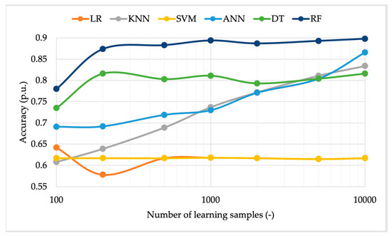
Figure 6.
Algorithm accuracy vs. the number of learning samples using uniform distributed inputs.
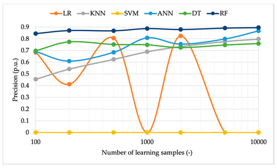
Figure 7.
Algorithm precision vs. the number of learning samples using uniform distributed inputs.
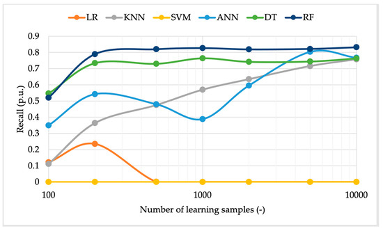
Figure 8.
Algorithm recall vs. the number of learning samples using uniform distributed inputs.
Another important conclusion from Figure 6 is that there is no need to use a massive number of samples for the learning stage. In the plotted case, already at 1000 samples, almost all the algorithms reach their maximum accuracy.
Regarding the precision graph depicted in Figure 7, some similar comments are made. In terms of absolute value, the RF and ANN are still the best ones, even if the gap with KNN and DT is reduced compared to the accuracy case. Focusing on the performance of the LR algorithm, it fluctuates as the number of input samples changes. This is because the algorithm performance, in addition to the overall number of learning samples, also depends on the percentage of faulty cases among them. Thus, if the total number of input samples is increased, it is not obvious that the performance will also have the same behavior. Finally, the SVM is clearly the worst-performing algorithm. Comparing accuracy and precision, it can be observed that the first metric is not null, since the algorithm can correctly identify all the TN cases of the test set (a percentage equal to the value of accuracy). On the other hand, the precision is null because there are zero TP cases identified by the SVM.
Note that the comment on the tradeoff between precision and the number of samples is analogous to the accuracy case, demonstrating that the use of 1000 samples is still a valid option.
In Figure 8, the recall metric is plotted. No additional comments are needed for the algorithms KNN, ANN, DT, and RF. The only observation to add is that their recall tends to the same value as the number of samples increases. Regarding the LR and SVM, these algorithms are still the worst ones.
By relating precision and recall, it can be generally observed that, if the precision is zero, the recall must also be zero. Conversely, if the precision is not null, neither is the recall. Regarding the LR algorithm, when it has acceptable precision values, it has recall values close to zero. The explanation for this behavior is that the metric of precision has, in the denominator, the number of FP cases (a small number, since this algorithm almost always returns 0 as an output), while the metric of recall has the number of FN cases (a large number, for the same reason mentioned before).
Evaluating the recall trend of the SVM, this is instead always null because the precision of the algorithm has the same trend.
Overall, considering the contributions provided in the previous three figures, it can be concluded that using 1000 samples for the learning stage is the best option. Furthermore, a limited number of samples (i) reduces the time required for the learning stage; (ii) allows the SOs to minimize the data to be used in that stage, focusing only on the testing one; and (iii) reduces the computational burden.
In light of the choice to adopt 1000 samples, Figure 9 collects the metrics of the accuracy, precision, and recall of all ML algorithms, tested with 1000 samples. This allows for a direct comparison of the performance of the algorithms.
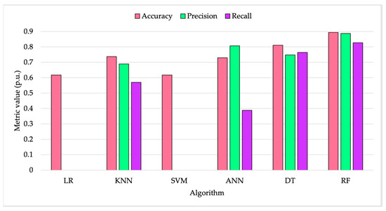
Figure 9.
Algorithm metrics in the case of 1000 samples for the learning stage.
6.2. Repeatability
In Table 3, the results of the repeatability test are listed. For each algorithm, the mean value of the accuracy obtained with 500 repetitions and the associated standard deviation are given. Note that the tests have been run with 1000 samples for the learning stage and considering uniformly distributed data. From the results, the almost negligible variations confirm the repeatability of the algorithms.
Table 3.
Mean and standard deviation values of algorithms executed 500 times.
6.3. Data Distribution
The results in this section assess the usage of normally distributed input data. Analogously to Section 6.1, Figure 10, Figure 11 and Figure 12, respectively, graph the algorithm metrics of accuracy, precision, and recall versus the number of learning samples.
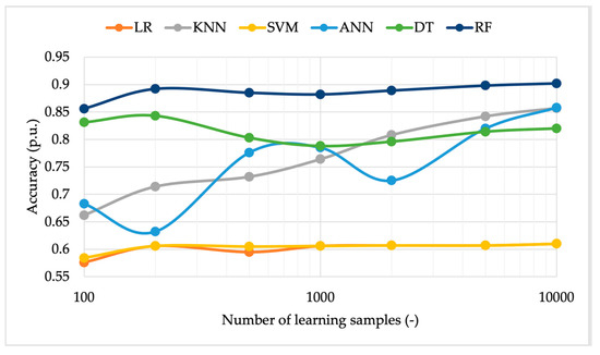
Figure 10.
Algorithm accuracy vs. the number of learning samples using normal distributed inputs.
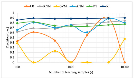
Figure 11.
Algorithm precision vs. the number of learning samples using normal distributed inputs.
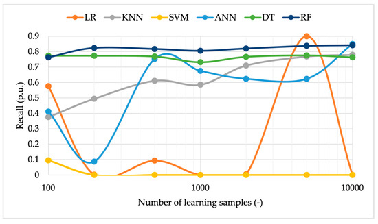
Figure 12.
Algorithm recall vs. the number of learning samples using normal distributed inputs.
In Figure 10, accuracy can be observed. Its behavior is almost identical to the one obtained from uniformly distributed samples. The algorithms, though, can be considered independent, in terms of accuracy, of the distribution assumed by the input data.
The same comments can be extended to the precision and recall in Figure 11 and Figure 12. The two metrics are not affected by the change in the adopted distribution. A further comment can be made on the accuracy resulting from tests performed with a limited number of samples. From the graphs, a generally improved behavior of the metrics, compared to the uniform distribution case, between 100 and 500 samples emerges.
Considering that no significant variations have been obtained from the implementation of normally distributed samples, the 1000 sample choice is still valid. Therefore, Figure 13 shows the value of the three metrics of each algorithm tested with 1000 samples in the learning stage.
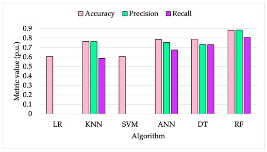
Figure 13.
Algorithm metrics in the case of 1000 normally distributed samples.
6.4. Uncertainty
To evaluate the influence of uncertainty on the performance of the algorithms, the histogram graphed in Figure 14 shows the metrics obtained with and without the application of the 10% uncertainty contribution. Each test has been executed with uniformly distributed input data and 1000 samples for the learning stage.
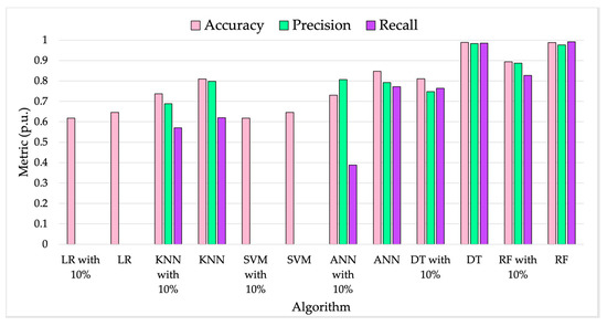
Figure 14.
Algorithm metrics with and without the application of the 10% uncertainty contribution, with uniform distributed inputs.
From the graph, it can be concluded that, as expected, the uncertainty contribution affects all the evaluated metrics. Hence, the reliability of the input data is a critical aspect to consider, and it is worth further studying.
6.5. Percentage of Faults
Each SO might have different fault rates depending on the various conditions of their network. Therefore, it is useful to test the efficiency of the ML algorithms, varying the number of faults in the learning stage. The testing results are collected in Table 4. It includes, for each algorithm, the accuracy (A), the precision (P), and the recall (R) obtained with 5%, 10%, 25%, and 50% of faults. Three colors have been used to better distinguish between A, P, and R.
Table 4.
Metrics vs. percentage of the faults in the learning set.
According to the results, some algorithms, such as DT and RF, are not affected by variations in the number of faults in the learning test. These two algorithms perform well in all conditions, and it is reflected in the three metrics. As for ANN and KNN, their performance slightly increases with the increase in the percentage, providing the best results with 50% of faulty cases. Finally, LR and SVM do not perform well in any of the cases, showing better results only for precision and recall in the 50% case. However, this result was expected considering the underfitting problems highlighted in the previous tests.
6.6. Computational Burden
As mentioned before, another critical parameter for the evaluation of an algorithm is the computational burden. It is assessed in terms of the time required by the algorithm to complete the analysis. For this purpose, the execution times of the algorithms are reported in Table 5. In addition to the times in the table, 0.978 s are needed to generate the synthetic dataset consisting of 1000 and 100,000 samples for the learning and the testing stage, respectively.
Table 5.
Algorithm execution times.
The table highlights significant discrepancies among the algorithms. There are more than 6 s of difference between the LR and SVM algorithms. However, the most promising algorithms tested in this paper do not exceed 2 s. Such a value is acceptable considering the fault prediction for the cable joint scenario.
6.7. Final Considerations
After detailing all the results, it is necessary to summarize the achievements and comment on them.
First, the goal of this work is to assess (and stress) several ML algorithms to understand their applicability to the fault prediction of MV cable joints. The idea is that AI can provide precious information on the health status of the cable joint. Therefore, algorithms have been compared not only from the perspective of their performance but also considering the SO’s perspective. In this way, SOs may easily implement the algorithm(s) in their control rooms to collect and compute the measures collected from the field.
For this purpose, the case study simulates an actual distributed measurement system that allows for the collection of several quantities from the cable joint. Afterwards, the measures are processed by the ML algorithms. Note that the critical aspect is associating a “fault risk” with a set of measured parameters (the definition of thresholds). To date, there is no standard literature or common agreement about the exact conditions and parameter combinations that lead to a fault in an MV cable joint. Furthermore, every SO will collect measures from the field before a fault, reflecting different conditions. Therefore, the algorithms and the simulated thresholds used in this work are based on the authors’ expertise and experience.
Looking at the results, it is possible to conclude that:
- The application of ML algorithms to the fault prediction of MV cable joints is promising.
- Each algorithm has specific peculiarities; hence, they are not all suitable for the considered application. However, DT and RF can be considered the top-performing algorithms.
- The selection of the algorithm highly depends on the computational burden that is sustainable by the SO. From another perspective, it depends on the extension of the considered grid or the number of deployed sensors.
- The success of the algorithm, once selected, strongly depends on the input data and the choices made from experience.
- The uncertainty of the input data, more than the uncertainty of the algorithm results, affects the validity of the results.
Overall, there is no need to select the perfect algorithm. It is more significant to highlight each of their peculiarities, allowing the final users to make the best decision depending on their requirements.
7. Conclusions
This work aims to provide a complete study, even if the topic is emerging, on the selection of ML algorithms. It has been necessary to fill in a gap in the literature, providing the correct tools to the final users. For this purpose, a realistic case study, based on the simulation of distributed measurement systems, has been designed. The simulated measurement results were then used to compare the performance of six ML algorithms. The aim of the comparison is the algorithms’ applicability to the fault prediction of the MV cable joints. In detail, AI can provide precious information on the health status of cable joints. Different aspects have been tested, not only the simple algorithm accuracy. The results provide information on the algorithm performance, the number of samples to be used, and the computational burden of the algorithms. Finally, the quality of the results triggers several further studies that will be completed in the future.
Author Contributions
Conceptualization, A.M.; methodology, R.T.; software, V.N.; validation, V.N.; resources, L.P.; writing—original draft preparation, A.M.; writing—review and editing, R.T.; supervision, L.P. All authors have read and agreed to the published version of the manuscript.
Funding
This research received no external funding.
Data Availability Statement
Not applicable.
Conflicts of Interest
The authors declare no conflict of interest.
References
- Holma, A.; Leskinen, P.; Myllyviita, T.; Manninen, K.; Sokka, L.; Sinkko, T.; Pasanen, K. Environmental impacts and risks of the national renewable energy targets—A review and a qualitative case study from finland. Renew. Sustain. Energy Rev. 2018, 82, 1433–1441. [Google Scholar] [CrossRef]
- Kabir, Z.; Sultana, N.; Khan, I. Environmental, social, and economic impacts of renewable energy sources. In Renewable Energy and Sustainability: Prospects in the Developing Economies; Elsevier: Amsterdam, The Netherlands, 2022; pp. 57–85. [Google Scholar] [CrossRef]
- Pratiwi, S.; Juerges, N. Review of the impact of renewable energy development on the environment and nature conservation in southeast asia. Energy Ecol. Environ. 2020, 5, 221–239. [Google Scholar] [CrossRef]
- Meneguzzo, F.; Ciriminna, R.; Albanese, L.; Pagliaro, M. The remarkable impact of renewable energy generation in sicily onto electricity price formation in italy. Energy Sci. Eng. 2016, 4, 194–204. [Google Scholar] [CrossRef]
- Niu, S.; Zhang, Z.; Ke, X.; Zhang, G.; Huo, C.; Qin, B. Impact of renewable energy penetration rate on power system transient voltage stability. Energy Rep. 2022, 8, 487–492. [Google Scholar] [CrossRef]
- Pearre, N.S.; Swan, L.G. Extensible electricity system model for high penetration rate renewable integration impact analysis. J. Energy Eng. 2014, 140, 04013003. [Google Scholar] [CrossRef]
- Winkler, J.; Gaio, A.; Pfluger, B.; Ragwitz, M. Impact of renewables on electricity markets—Do support schemes matter? Energy Policy 2016, 93, 157–167. [Google Scholar] [CrossRef]
- Gray, M.K.; Morsi, W.G. On the impact of single-phase plug-in electric vehicles charging and rooftop solar photovoltaic on distribution transformer aging. Electr. Power Syst. Res. 2017, 148, 202–209. [Google Scholar] [CrossRef]
- Jones, C.B.; Lave, M.; Vining, W.; Garcia, B.M. Uncontrolled electric vehicle charging impacts on distribution electric power systems with primarily residential, commercial or industrial loads. Energies 2021, 14, 1688. [Google Scholar] [CrossRef]
- Leou, R.; Su, C.; Lu, C. Stochastic analyses of electric vehicle charging impacts on distribution network. IEEE Trans. Power Syst. 2014, 29, 1055–1063. [Google Scholar] [CrossRef]
- Vagropoulos, S.I.; Balaskas, G.A.; Bakirtzis, A.G. An investigation of plug-in electric vehicle charging impact on power systems scheduling and energy costs. IEEE Trans. Power Syst. 2017, 32, 1902–1912. [Google Scholar] [CrossRef]
- IEC 61869-10; Part 10: Additional Requirements for Low-Power Passive Current Transformers: Instrument Transformers. International Standardization Organization: Geneva, Switzerland, 2018.
- IEC 61869-11:2018; Instrument transformers—Part 11: Additional requirements for low-power passive voltage transformers. International Standardization Organization: Geneva, Switzerland, 2018.
- Crotti, G.; Femine, A.D.; Gallo, D.; Giordano, D.; Landi, C.; Letizia, P.S.; Luiso, M. Traceable characterization of low power voltage instrument transformers for PQ and PMU applicationsIn Proceedings of the CPEM Digest Conference on Precision Electromagnetic Measurements, Denver, CO, USA, 24–28 August 2020. [CrossRef]
- Mingotti, A.; Bartolomei, L.; Peretto, L.; Tinarelli, R. On the long-period accuracy behavior of inductive and low-power instrument transformers. Sensors 2020, 20, 810. [Google Scholar] [CrossRef] [PubMed]
- Normandeau, M.; Mahseredjian, J. Evaluation of low-power instrument transformers for generator differential protection. IEEE Trans. Power Delivery 2018, 33, 1143–1152. [Google Scholar] [CrossRef]
- Veinovic, S.; Ponjavic, M.; Milic, S.; Djuric, R. Low-power design for DC current transformer using class-D compensating amplifier. IET Circuits Devices Syst. 2018, 12, 215–220. [Google Scholar] [CrossRef]
- Jalal, S.; Nicolaou, S.; Parker, W. Artificial intelligence, radiology, and the way forward. Can. Assoc. Radiol. J. 2019, 70, 10–12. [Google Scholar] [CrossRef]
- Qu, J.; Zhao, Y.; Xie, Y. Artificial intelligence leads the reform of education models. Syst. Res. Behav. Sci. 2022, 39, 581–588. [Google Scholar] [CrossRef]
- Shanthi, V.; Pavithra, R. A study relating to the application and use of artificial intelligence in the banking sector. Int. J. Adv. Sci. Technol. 2020, 29, 797–802. [Google Scholar]
- Zhou, J.; Shen, M. When human intelligence meets artificial intelligence. PsyCh J. 2018, 7, 156–157. [Google Scholar] [CrossRef]
- Chandrasekaran, K.; Selvaraj, J.; Xavier, F.J.; Kandasamy, P. Artificial neural network integrated with bio-inspired approach for optimal VAr management and voltage profile enhancement in grid system. Energy Sources Part A Recovery Util. Environ. Eff. 2021, 43, 2838–2859. [Google Scholar] [CrossRef]
- Della Krachai, S.; Boudghene Stambouli, A.; Della Krachai, M.; Bekhti, M. Experimental investigation of artificial intelligence applied in MPPT techniques. Int. J. Power Electron. Drive Syst. 2019, 10, 2138–2147. [Google Scholar] [CrossRef]
- Gastalver-Rubio, A.; Carmona-Pardo, R. Application of neural networks to determine the customer connectivity based on smart meters. Renew. Energy Power Qual. J. 2020, 18, 8–12. [Google Scholar] [CrossRef]
- Kurokawa, F.; Tanaka, M.; Furukawa, Y.; Matsui, N. Recent research trends of artificial intelligence applications in power electronics. Int. J. Renew. Energy Res. 2021, 11, 1370–1381. [Google Scholar]
- Tzimas, A.; Diban, B.; Boyer, L.; Chen, G.; Castellon, J.; Chitiris, N.; Wu, K. Feasibility of space charge measurements on HVDC cable joints: Study group-IEEE DEIS technical committee HVDC cable and systems. IEEE Electr. Insul. Mag. 2022, 38, 18–27. [Google Scholar] [CrossRef]
- Winkelmann, E.; Shevchenko, I.; Steiner, C.; Kleiner, C.; Kaltenborn, U.; Birkholz, P.; Steiner, T. Monitoring of partial discharges in HVDC power cables. IEEE Electr. Insul. Mag. 2022, 38, 7–18. [Google Scholar] [CrossRef]
- Zhang, L.; Yang, X.L.; Le, Y.; Yang, F.; Gan, C.; Zhang, Y. A thermal probability density-based method to detect the internal defects of power cable joints. Energies 2018, 11, 1674. [Google Scholar] [CrossRef]
- Negri, V.; Mingotti, A.; Peretto, L.; Tinarelli, R. Artificial Intelligence and Smart Grids: The Cable Joint Test Case. In Proceedings of the 2022 IEEE 12th International Workshop on Applied Measurements for Power Systems (AMPS), Cagliari, Italy, 28–30 September 2022; pp. 1–6. [Google Scholar]
- Martinez, R. Artificial Intelligence: Distinguishing between Types & Definitions. Nev. Law J. 2019, 19, 1015–1042. [Google Scholar]
- El Mrabet, M.; El Makkaoui, K.; Faize, A. Supervised Machine Learning: A Survey. In Proceedings of the 2021 4th International Conference on Advanced Communication Technologies and Networking (CommNet), Rabat, Morocco, 3–5 December 2021; pp. 1–10. [Google Scholar] [CrossRef]
- Vladimir, N. An overview of the supervised machine learning methods. Horizons 2017, 4, 51–62. [Google Scholar]
- Cervantes, J.; Garcia-Lamont, F.; Rodríguez-Mazahua, L.; Lopez, A. A comprehensive survey on support vector machine classification: Applications, challenges and trends. Neurocomputing 2020, 408, 189–215. [Google Scholar] [CrossRef]
- Guo, G.; Wang, H.; Bell, D.; Bi, Y.; Greer, K. KNN Model-Based Approach in Classification. In On The Move to Meaningful Internet Systems 2003: CoopIS, DOA, and ODBASE OTM, Proceedings of the Confederated International Conferences CoopIS, DOA, and ODBASE 2003, Catania, Sicily, Italy, November 3–7, 2003; Lecture Notes in Computer Science; Meersman, R., Tari, Z., Schmidt, D.C., Eds.; Springer: Berlin/Heidelberg, Germany, 2003; Volume 2888. [Google Scholar] [CrossRef]
- Schonlau, M.; Zou, R.Y. The random forest algorithm for statistical learning. Stata J. 2020, 20, 3–29. [Google Scholar] [CrossRef]
- Rajni, B.; Kumar, D.A. Classification Using ANN: A Review. Int. J. Comput. Intell. Res. 2017, 13, 1811–1820. [Google Scholar]
- Rana, K.; Dasgupta, B. Analysis of HT cable and joint failures and associated design modifications. In Third-Party Damage to Underground and Submarine Cables; CIGRE Working Group B1.21; CIGRE: Paris, France, 2009. [Google Scholar]
- Allen, R.W., Jr.; Burnup, E.C., Jr.; Medek, J.; Mulligan, J.; Sacks, N.; Schneider, G. Analysis of joint & termination failures on extruded dielectric cables. IEEE Trans. Power Appar. Syst. 1984, 103, 3464–3469. [Google Scholar]
- Dong, X.; Yuan, Y.; Gao, Z.; Zhou, C.; Wallace, P.; Alkali, B.; Sheng, B.; Zhou, H. Analysis of cable failure modes and cable joint failure detection via sheath circulating current. In Proceedings of the Electrical Insulation Conference, Philadelphia, PA, USA, 8–11 June 2014. [Google Scholar]
- Jiang, Y.; Min, H.; Luo, J.; Li, Y.; Jiang, X.; Xia, R.; Li, W. Partial Discharge Pattern Characteristic of HV Cable Joints with Typical Artificial Defect. In Proceedings of the 2010 Asia-Pacific Power and Energy Engineering Conference, Chendu, China, 28–31 March 2010. [Google Scholar]
- Testa, L.; Cavallini, A.; Montanari, G.C.; Makovoz, A. On-line partial discharges monitoring of high voltage XLPE/fluid-filled transition joints. In Proceedings of the Electrical Insulation Conference, Annapolis, MD, USA, 5–8 June 2011. [Google Scholar]
- Rajalakshmi, B.; Kalaivani, L. Analysis of Partial Discharge in underground cable joints. In Proceedings of the International Conference on Innovations in Information, Embedded and Communciation Systems, Coimbatore, India, 19–20 March 2015. [Google Scholar]
- Wu, R.; Chang, C.K. The Use of Partial Discharges as an Online Monitoring System for Underground Cable Joints. IEEE Trans. Power Deliv. 2011, 24, 1585–1591. [Google Scholar] [CrossRef]
- Fournier, D.; Lamarre, L. Effect of pressure and temperature on interfacial breakdown between two dielectric surfaces. In Proceedings of the Conference on Electrical Insulation and Dielectric Phenomena, Victoria, BC, Canada, 18–21October 1992; pp. 229–235. [Google Scholar]
- Zhou, X.; Cao, J.; Wang, S.; Jiang, Y.; Li, T.; Zou, Y. Simulation of electric field around typical defects in 110kV XLPE power cable joints. In Proceedings of the 2017 International Conference on Circuits, Devices and Systems (ICCDS), Chengdu, China, 5–8 September 2017; pp. 21–24. [Google Scholar]
- Permal, N.; Chakrabarty, C.; Avinash, A.R.; Marie, T.; Halim, H.S.A. Tangent Delta Extraction of Cable Joints for Aged 11kV Underground Cable System. In Proceedings of the International Conference on Advances in Electrical Electronic and System Engineering, Putrajaya, Malaysia, 14–16 November 2016. [Google Scholar]
- Mingotti, A.; Ghaderi, A.; Peretto, L.; Tinarell, R.; Lama, F. Test Setup Design, and Calibration for Tan Delta Measurements on MV Cable Joints. In Proceedings of the 2018 IEEE 9th International Workshop on Applied Measurements for Power Systems (AMPS), Bologna, Italy, 26–28 September 2018; pp. 1–5. [Google Scholar]
- Ghaderi, A.; Mingotti, A.; Lama, F.; Peretto, L.; Tinarelli, R. Effects of Temperature on MV Cable Joints Tan Delta Measurements. IEEE Trans. Instrum. Meas. 2019, 68, 3892–3898. [Google Scholar] [CrossRef]
- Ghaderi, A.; Mingotti, A.; Peretto, L.; Tinarelli, R. Effects of Mechanical Pressure on the Tangent Delta of MV Cable Joints. IEEE Trans. Instrum. Meas. 2019, 68, 2656–2658. [Google Scholar] [CrossRef]
- Di Sante, R.; Ghaderi, A.; Mingotti, A.; Peretto, L.; Tinarelli, R. Test Bed Characterization for the Interfacial Pressure vs. Temperature Measurements in MV Cable-Joints. In Proceedings of the 2019 II Workshop on Metrology for Industry 4.0 and IoT (MetroInd4.0&IoT), Naples, Italy, 4–6 June 2019; pp. 186–190. [Google Scholar]
- Di Sante, R.; Ghaderi, A.; Mingotti, A.; Peretto, L.; Tinarelli, R. Effects of Thermal Cycles on Interfacial Pressure in MV Cable Joints. Sensors 2019, 20, 169. [Google Scholar] [CrossRef]
- Gulski, J.R.; Smit, J. Failures of medium voltage cable joints in relation to the ambient temperature. In Proceedings of the 20th International Conference on Electricity Distribution, Prague, Czech Republic, 8–11 June 2009. [Google Scholar]
- scikitLearn. Available online: https://scikit-learn.org/stable/user_guide.html (accessed on 10 November 2022).
- Choudhary, R.; Gianey, H.K. Comprehensive Review On Supervised Machine Learning Algorithms. In Proceedings of the 2017 International Conference on Machine Learning and Data Science (MLDS), Noida, India, 14–15 December 2017; pp. 37–43. [Google Scholar] [CrossRef]
- ISO/IEC Guide 98-3:2008; Uncertainty of Measurement—Part 3: Guide to the Expression of Uncertainty in Measurement (GUM:1995). International Standardization Organization: Geneva, Switzerland, 2008.
Disclaimer/Publisher’s Note: The statements, opinions and data contained in all publications are solely those of the individual author(s) and contributor(s) and not of MDPI and/or the editor(s). MDPI and/or the editor(s) disclaim responsibility for any injury to people or property resulting from any ideas, methods, instructions or products referred to in the content. |
© 2023 by the authors. Licensee MDPI, Basel, Switzerland. This article is an open access article distributed under the terms and conditions of the Creative Commons Attribution (CC BY) license (https://creativecommons.org/licenses/by/4.0/).