Article

Analysis of Interturn Faults on Transformer Based on Electromagnetic-Mechanical Coupling

1
School of Electrical Engineering and Automation, Tianjin University of Technology, Tianjin 300384, China
2
Tianjin Key Laboratory for Control Theory & Application in Complicated Systems, Tianjin 300384, China
*
Authors to whom correspondence should be addressed.
Energies 2023, 16(1), 512; https://doi.org/10.3390/en16010512
Submission received: 29 November 2022 / Revised: 26 December 2022 / Accepted: 29 December 2022 / Published: 2 January 2023

Abstract

:
A running transformer frequently experiences interturn faults; they are typically difficult to detect in their early stages but eventually progress to interturn short circuits, which cause damage to the transformer. Therefore, finding out the fault mechanism of the full interturn fault process can provide a theoretical basis for transformer fault detection. In this paper, an electromagnetic-solid mechanics coupled finite element model consistent with an actual oil-immersed three-phase transformer is established. The transient process of winding from interturn discharge to interturn short circuit is simulated to study the electromagnetic characteristics as well as the mechanical characteristics during transformer failure. The model parameters of the transformer are simulated to obtain the fault current, electromagnetic parameters and other performance parameters to study the characteristics of the magnetic field and coil force when interturn faults occur. Finally, the vibration of the transformer casing is used to detect as well as diagnose the transformer fault situation, providing a theoretical basis for the study of transformer detection and diagnosis capability improvement measures.

1. Introduction

The interturn fault is one of the common faults of oil–immersed power transformers, while the winding interturn insulation aging and continuous partial discharge is the main cause of interturn faults. Partial discharge occurs between the windings at the beginning of a transformer interturn fault. As the insulation material between the windings ages, the interturn insulation resistance decreases. Partial discharge occurs between windings at the initial stage of transformer turn–to–turn fault. As the insulation material between the windings ages, the inter–turn insulation resistance decreases. After the development of inter–turn discharge to a certain extent, the insulation between the transformer windings will be penetrated resulting in infinitesimal insulation resistance, thus occurring between the turns of the winding short circuit [1]. Significant electromagnetic forces are generated in the event of a transformer turn–to–turn short circuit, which can lead to elastic and plastic deformation of the transformer windings and catastrophic failure of the transformer [2]. Transformer failures due to short–circuit forces are a major concern for transformer users [3], and much literature has been devoted to the insulation design of transformers and to the calculation of leakage inductance as a means of reducing hysteresis losses and reducing short–circuit electromagnetic forces [4]. Thus, the problem of how to find and stop interturn faults in transformers needs to be solved.
The experimental analysis of interturn faults in operating transformers is typically challenging, and experiments cannot measure detailed data during transformer fault operation. Therefore, a combination of finite element software is needed to simulate the transient process of multi–physics field coupling in transformers. At present, the research on the simulation of transformer winding interturn short circuit fault is mainly on the electromagnetic characteristics and mechanical characteristics after an interturn short circuit [5]. In recent years, many scholars have studied the characteristic parameters and characteristics of power transformer winding interturn short–circuit faults. In [6], a two–dimensional simulation model of a three–phase transformer is made to find out what happens in a running transformer when an interturn short–circuit fault happens. The results show that the terminal current, the circulating current in the short–circuiting turns, and the electromagnetic flux inside the transformer can all be used as reliable monitoring parameters for detecting transformer faults. In [7], the finite element method is used to make a simplified three–dimensional model of a split–winding transformer so that the forces acting on the short–circuit winding and the distribution of the leakage magnetic field at different points along the low–voltage winding can be studied. The results show that interturn winding short circuits in certain places have a significant effect on the axial winding on the same core, and that the distorted leakage magnetic field causes the normal and short–circuit windings to have too much axial thrust and end thrust force.
In summary, the problem of an inter–turn short circuit in transformer windings has attracted extensive research, and finite element software has been applied to simulate inter–turn short circuits. However, not much literature exists on the fault conditions that occur in oil–immersed three–phase power transformers during the process from interturn discharge to interturn short circuit and on the leakage distribution, coil forces, and core and enclosure vibrations of the transformer when interturn faults occur. To come up with good ways to find transformer interturn faults, it is important to understand the electromagnetic and mechanical properties of transformers when they have interturn faults and to study how the transformer moves when it has interturn faults.
In this paper, a multi–physics field simulation model consistent with the actual transformer is established using finite element simulation software to simulate the transient process from interturn discharge to interturn short circuit for oil–immersed three–phase power transformers. The simulation study obtains the changes of electromagnetic, mechanical, and other physical parameters of the transformer during the fault to analyze the current, transformer leakage, winding force, and vibration of the core and enclosure to provide a theoretical basis for identifying and diagnosing the interturn fault.

2. Finite Element Model of the Faulty Transformer

Because of how they are used, the electrical properties of the dielectric materials in power transformers can change a lot over the course of their service lives. Strong electric fields that the transformer is exposed to are typically to blame for the deterioration and aging of the insulation. Figure 1 illustrates how the parallel equivalent circuit is commonly used to represent the electrical properties of interturn insulation material. The transformer windings’ internal faults will be simulated using this model. The resistance R eq shows how much active power is lost by the dielectric, and the capacitance C eq shows how much reactive power is lost [8].
Because the capacitance of the equivalent circuit is so low, the capacitive reactance is very high near the power frequency and can be ignored. Resistance decreases with the further deterioration of insulation properties. When the interturn equivalent resistance decreases, it leads to transformer interturn discharge [9]. Eventually, the insulation is completely damaged. When the interturn equivalent resistance is almost zero, it will lead to a short circuit between the turns of the transformer [10].

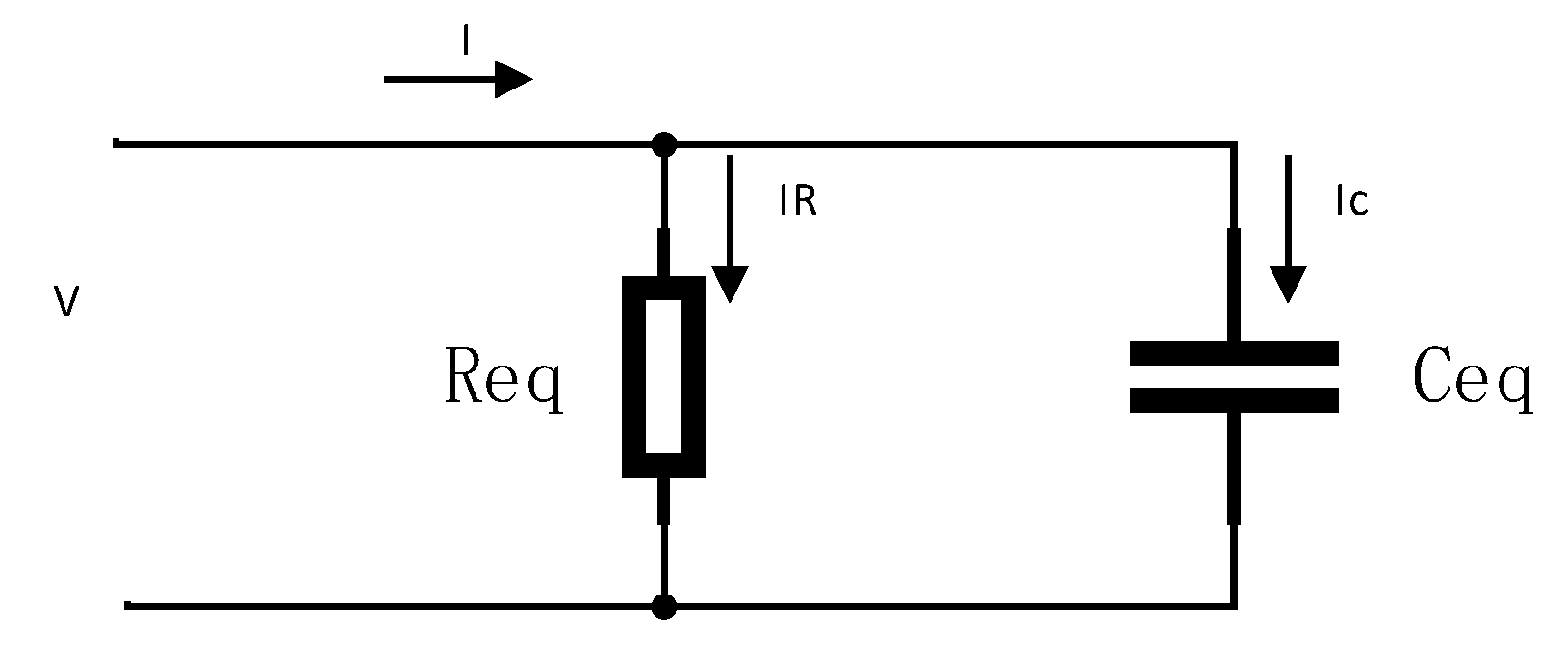
2.1. Electromagnetic Field Theory

Assuming that the transformer interturn fault occurs on the secondary side, an equivalent transformer interturn fault simulation circuit is created based on the equivalent circuit in Figure 1 [11]. The simulation circuit is shown in Figure 2, where R 1 represents the primary resistance, R 2 represents the secondary resistance, Z L represents the load, N 11 , N 12 , N 13 represent the high–voltage winding, N 21 , N 22 , N 23 represent the low–voltage winding, and N 22 represents the short–circuit winding [12].
The transformer winding will still satisfy Maxwell–Ampere’s law when an interturn fault occurs. The differential equations of the electromagnetic field can be obtained by associating Maxwell’s equations with the instantaneous equations as follows [6]:
× ( μ 0 1 μ r 1 × A ) + σ A t = J e
A is the vector magnetic potential, J e is the source current density, and μ r is the relative permeability, where μ 0 is the vacuum permeability.

2.2. Structural Mechanics Theory

In the finite element solid mechanics field coupling, Hooke’s law is used to find the relationship between strain and strain in a linear elastic material in the direction of the x–axis [13].
ε x = 1 E σ x v E ( σ y + σ z )
where ε x is the x–axis strain, E is the Young’s modulus of the transformer core, v is the Poisson’s ratio of the transformer core, and σ x , σ y , and σ z are the strain on the x–axis, y–axis and z–axis, respectively.
In the FEM analysis, since the strain and unit force equilibrium conditions need to be satisfied within each finite element so as to ensure the equilibrium of the whole model, the differential equation can be satisfied at any point of the iron core in the physical field of solid mechanics [14].
ρ 2 u t 2 = · S + F v
where u is the displacement vector at any point within the object, ρ is the object density, · S is the strain component in each direction at any point of the object, and F v is the physical place plus the body load.

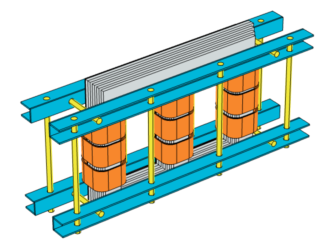
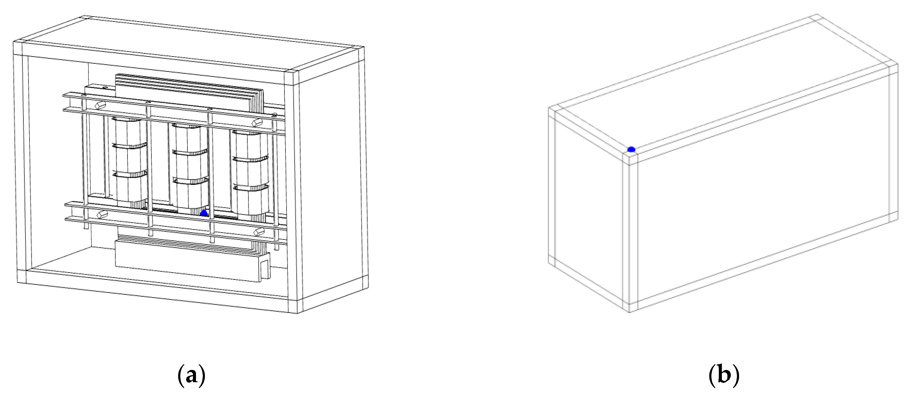
2.3. 3–D Model and Parameters of Power Transformer

In order to investigate the influence law of the physical characteristics of the transformer when inter–turn faults occur in the winding, this paper uses an oil–immersed three–phase transformer with a capacity of 100 kVA and a voltage of 10/0.4 kV as the object of study for simulation analysis. The main parameters are shown in Table 1.
The structure of power transformers is complex and includes a variety of components such as windings, cores and cooling devices. The model adds fasteners and enclosures according to the actual structure, which makes the simulation yield more accurate transformer vibration waveforms. For efficient simulation, components such as internal cooling units are therefore ignored. Based on the parameters of winding and core in Table 2 in the simulation software to build a three–dimensional model of the transformer, the model is shown in Figure 3.
Based on the above parameters and the simulation circuit in the simulation software to build a three–dimensional model of the transformer, the model is shown in Figure 3. The model adds fasteners according to the actual structure, which makes the simulation results more accurate.
The model draws the calculation area according to the actual oil–immersed transformer tank dimensions. The material property of the winding is set to copper, the core is selected as a loss–free soft iron, the relative dielectric constant of the transformer oil is 2.2, and the connection of the external circuit added in the winding is Yyn0 [15]. The termination time in the transient solver study setting is 500 ms and the time step is 0.5 ms. The solver used for the model is the default fully coupled transient solver. The finite element software adaptively divides the mesh area for the solution. The geometric model of the transformer is meshed by a free tetrahedral network. Finally, the boundary conditions in the physical field interface are set to build a coupled multi–physical field model for solution [13]. The established transformer fault model can be used to analyze the changes in current, leakage flux, electromagnetic force, and vibration at the core and transformer enclosure points under interturn faults in the transformer’s low–voltage side winding [16].

3. Analysis of Interturn Faults on Transformers Based on Electromagnetic Characteristics

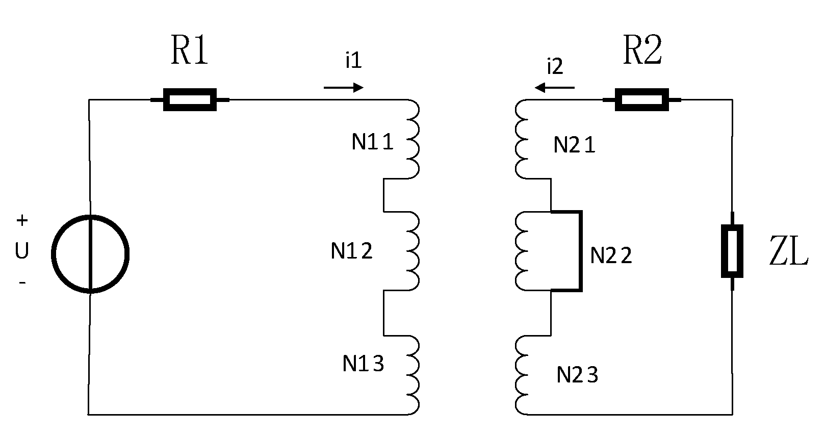
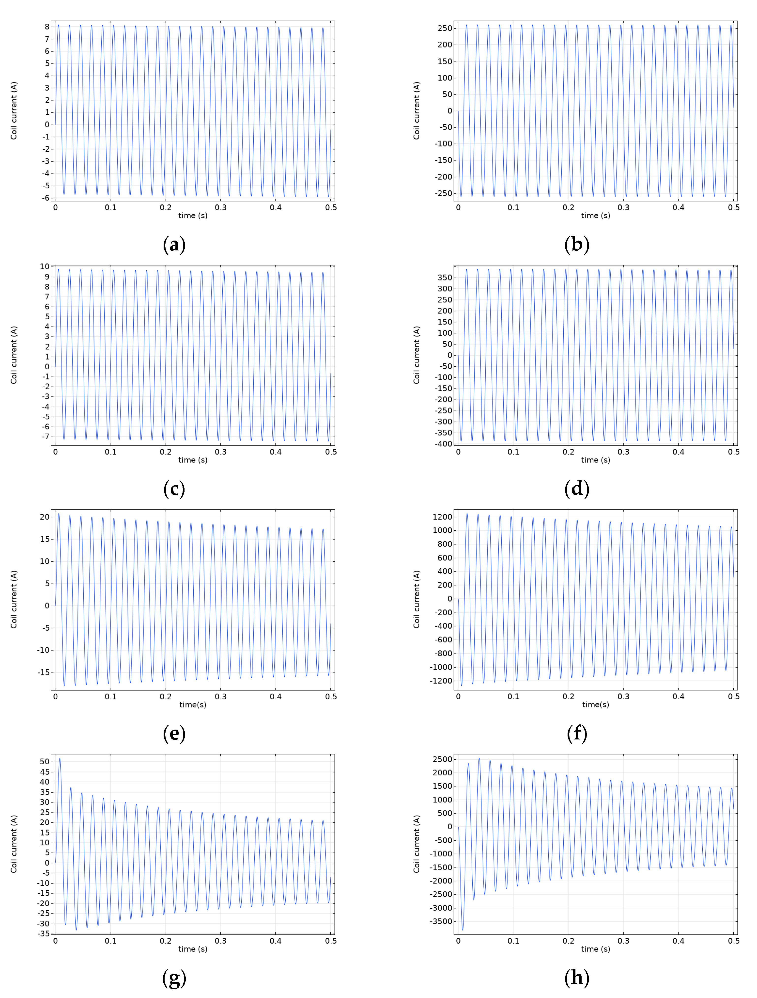
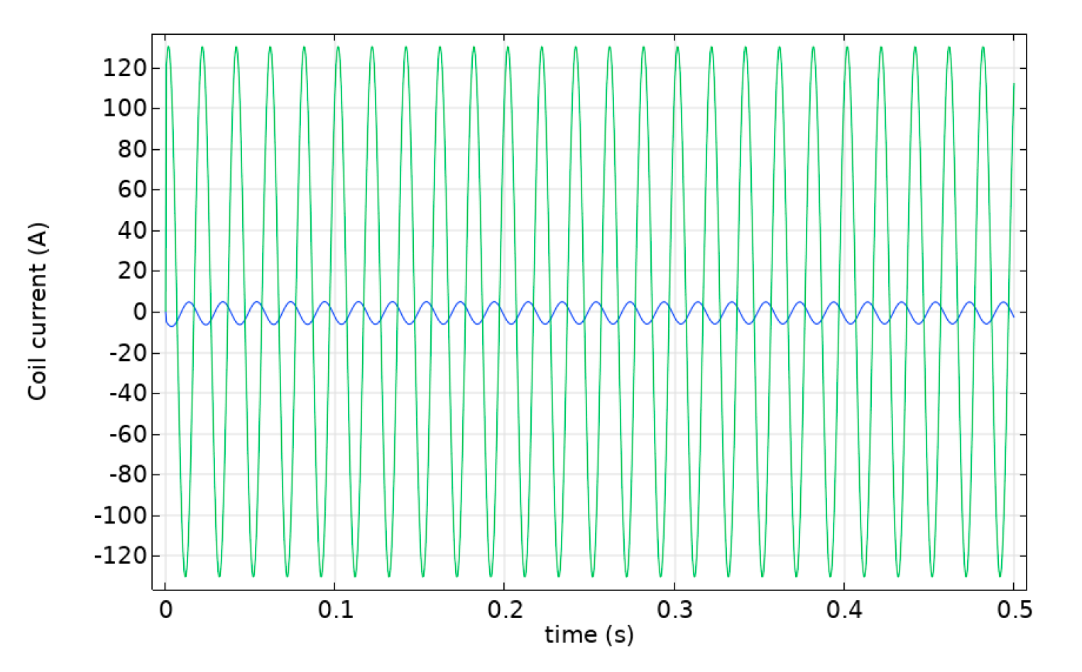
3.1. Winding Interturn Fault Current Analysis

Interturn faults are added to the simulation circuit of the transformer 3D model, and the fault is set to occur in the middle winding of the secondary side of phase B. The equivalent resistance used to simulate an interturn short circuit is generally less than 1   Ω . Therefore, the equivalent resistance is set to 1   Ω , 0.5   Ω , 0.1   Ω , and 0.01   Ω in turn, so as to simulate the transient process from interturn discharge to interturn short circuit [17].
A short circuit is created in the winding when an interturn fault happens. The minimum resistance of the winding is affected by the short–circuit loop’s induced voltage. Because the winding acts like an inductive element and the current does not change quickly, the short circuit has a circuit current that is much higher than the rated value.
Figure 4 and Figure 5 depict the primary and secondary side currents of the winding under normal and fault conditions, respectively. When inter–turn discharge occurs on the secondary side of the winding ( R eq = 1   Ω ), the fault current of the winding is about 260 A, which is about two times the normal winding current. However, as the equivalent resistance value of the faulty winding decreases, the fault current generated on the winding increases rapidly. When the insulation is completely damaged ( R eq = 0.01   Ω ), the short–circuit current of the winding is about 3800 A, which is tens of times the normal winding current.
It can be concluded that when an interturn fault happens in the secondary side fault winding, the primary winding must balance the flux produced by the fault current according to d Φ dt = 0 . As a result, the current in the primary winding rises. Due to the strong magnetic coupling between the primary and secondary sides, as the interturn fault gets worse, the current on the primary side is most affected. The increase in the secondary side fault current will lead to an increase in the primary side current as well, while the peak current on the primary side varies under different levels of faults.

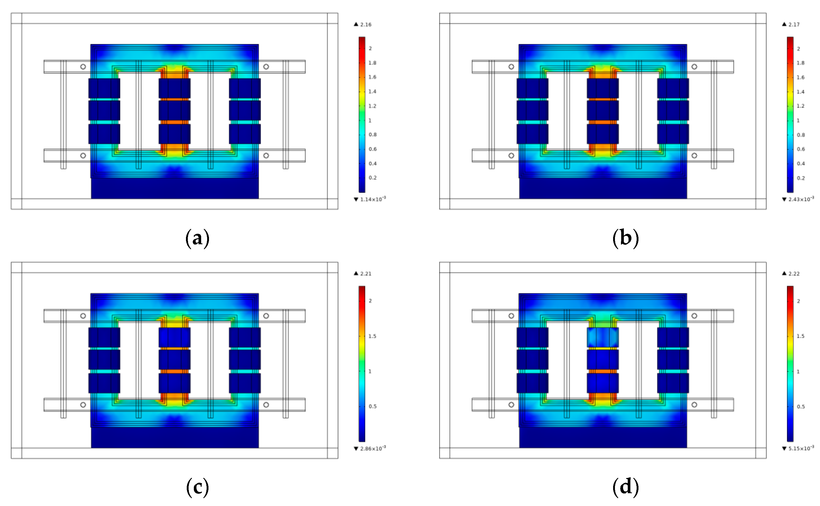
3.2. Magnetic Field Analysis

From the results of the first subsection, it can be seen that the winding becomes larger and larger during the inter–turn fault after the inter–turn fault occurs above the secondary side winding of phase B. The spatial magnetic field distribution will also change. To show how the flux density changes during a transformer interturn fault, the flux density diagrams of four different equivalent resistance models of the transformer at a certain point in the transient process are chosen.
Figure 6 shows how the resistance of the turn will go down as the magnetic flux around the short–circuit winding goes up. When the transformer has an interturn short circuit, the magnetic flux density on the surface of the bad winding can reach a maximum of about 0.8 T. The transformer’s total magnetic flux density distribution will have a higher maximum magnetic flux density, from 2.16 T to about 2.22 T. The transformer’s magnetic field’s maximum magnetic flux density will go from 1.92 T to about 1.98 T [18].
A cross–sectional analysis of the transformer’s flux density and magnetic field for the same time period as the interturn fault process is shown in Figure 6. It is easy to see how the flux density of the core near the faulty winding decreases and how the flux density of the said fault turns and the nearby leakage flux increases.
Therefore, it can be assumed that the presence of inter–turn faults causes the magnetic flux density of the core to become locally saturated. This, in turn, increases the leakage magnetic field near the short–circuit winding [19]. According to d Φ dt = 0 , when a winding interturn fault happens, the flux of the faulty winding will be cancelled out by the magnetic chains of the other windings [7]. The degree of leakage flux produced by the fault current is primarily responsible for the local saturation of the core flux density. However, when the leakage flux is very concentrated in the fault region, the symmetry of the leakage flux goes away.

4. Analysis of Interturn Faults on Transformers Based on Mechanical Characteristics

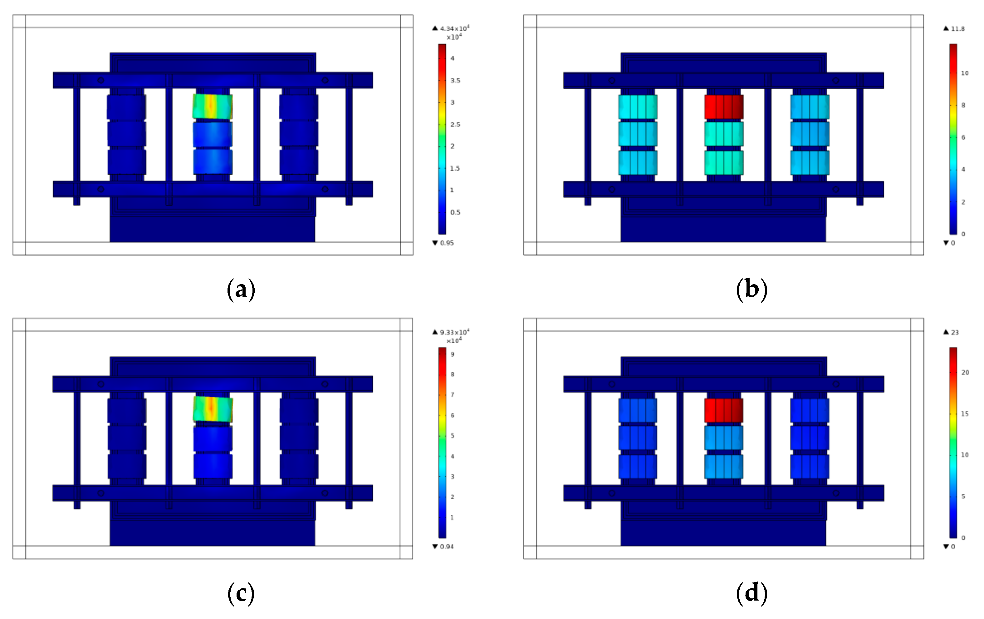
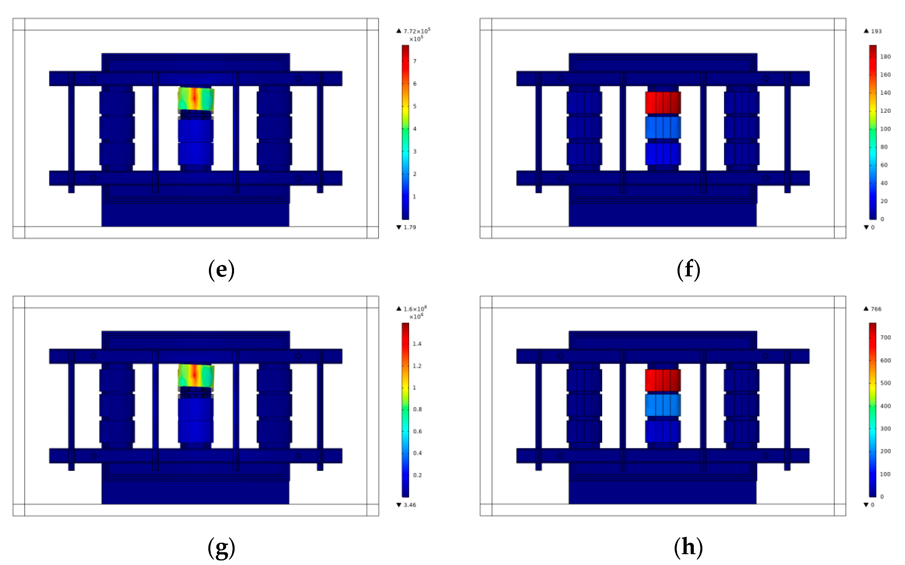
4.1. Analysis of Transformer Interturn Fault Force

The magnetic flux density of the transformer winding becomes larger after an interturn fault, which causes the strain on the faulty winding to become larger, resulting in the deformation of the shorted turn. In order to study the mechanical characteristics of a transformer after an interturn failure, the transformer in which the interturn failure occurred was coupled with solid mechanics for electromagnetic field–solid mechanics physical field coupling.
The results of the multi–physics field coupling simulation of the transformer are shown in Figure 7. It shows the transformer winding strain distribution and displacement during the process from interturn discharge to interturn short circuit. The strain on the transformer fault winding is relatively small when the equivalent resistance between turns is 1   Ω . The maximum strain on the fault winding is 4.34 × 10 4   N / m 2 , and the maximum deformation is 11.8 cm. The difference in stress and deformation magnitude between the faulty winding and the winding under normal conditions is about two times. However, as the interturn equivalent resistance decreases, when the interturn equivalent resistance is 0.01   Ω , the transformer short–circuit winding is subjected to a much larger force than the non–short–circuit winding, and the maximum strain on the coil is 2.67 × 10 5   N / m 2 , and the maximum deformation variable is 766   cm . Therefore, the deformation variable generated by the strain on the short–circuit winding can have a serious impact on the transformer operating condition [20].
It can be seen that the transformer in the occurrence of inter–turn failure of the fault winding current and magnetic flux density will become increasingly large so that the fault winding by the strain becomes larger. As the inter–turn insulation material ages until it is finally completely destroyed, the deformation of the faulty winding is several times higher than normal. After the deformation of the winding, the mechanical properties of the winding will be reduced. When the winding is impacted by the inter–turn fault current again, it is very likely that it will not be able to withstand the impact of the significant amount of power, and then the accident of damage will occur [21].

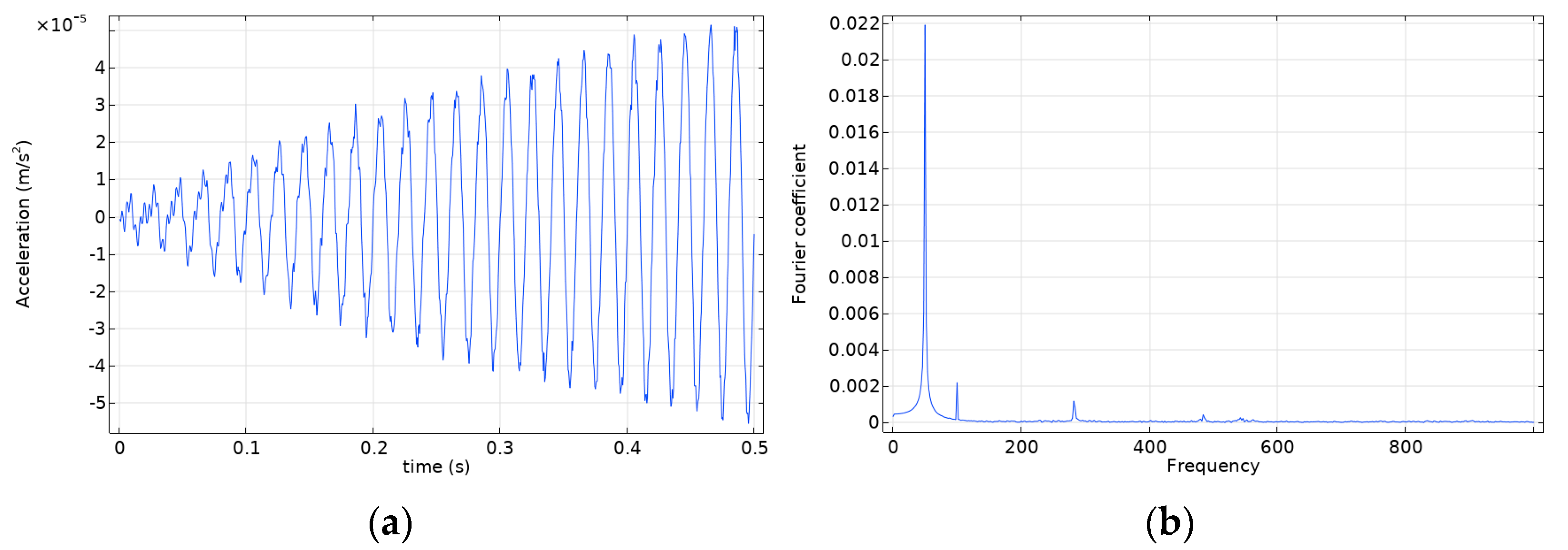
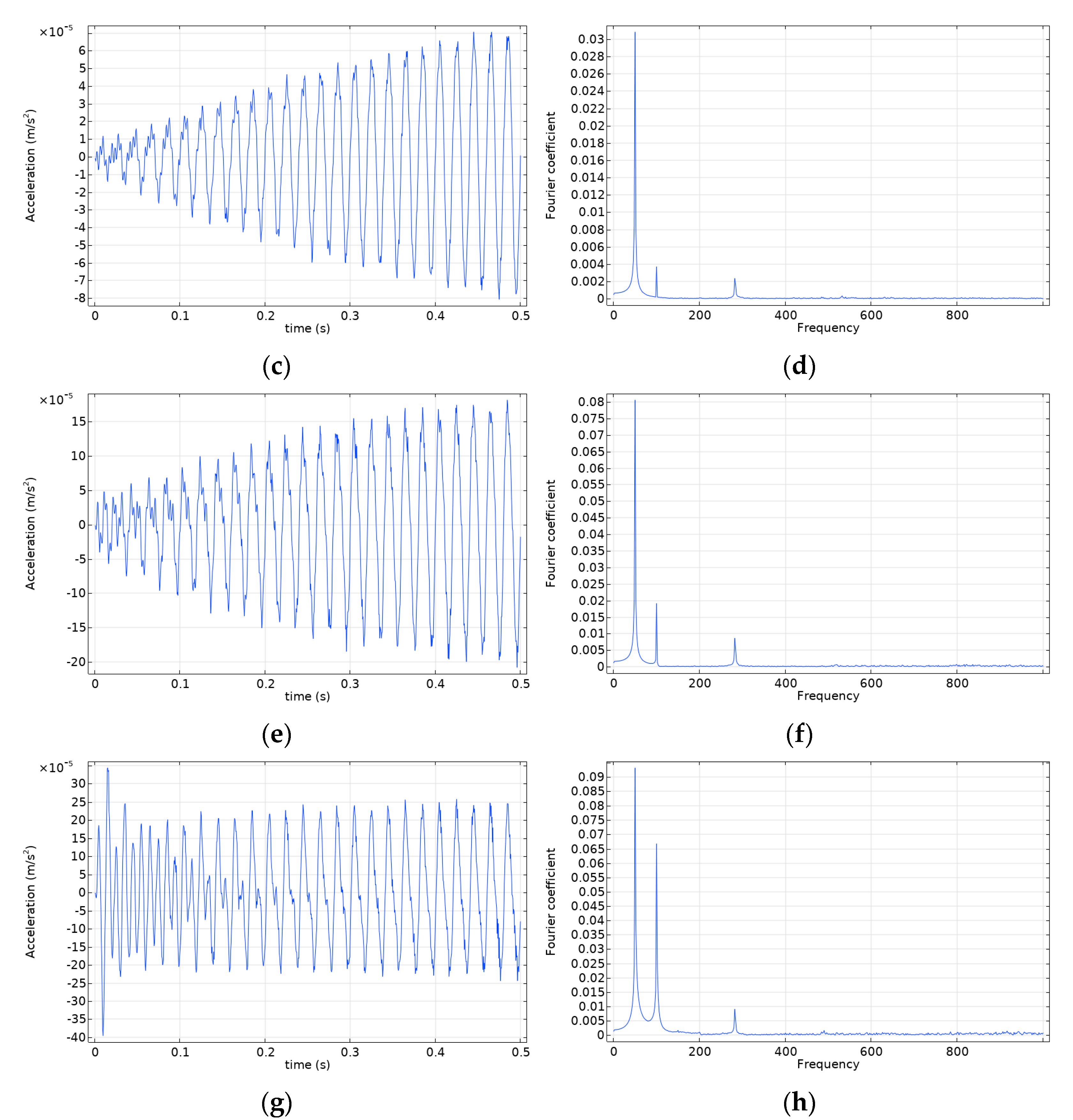
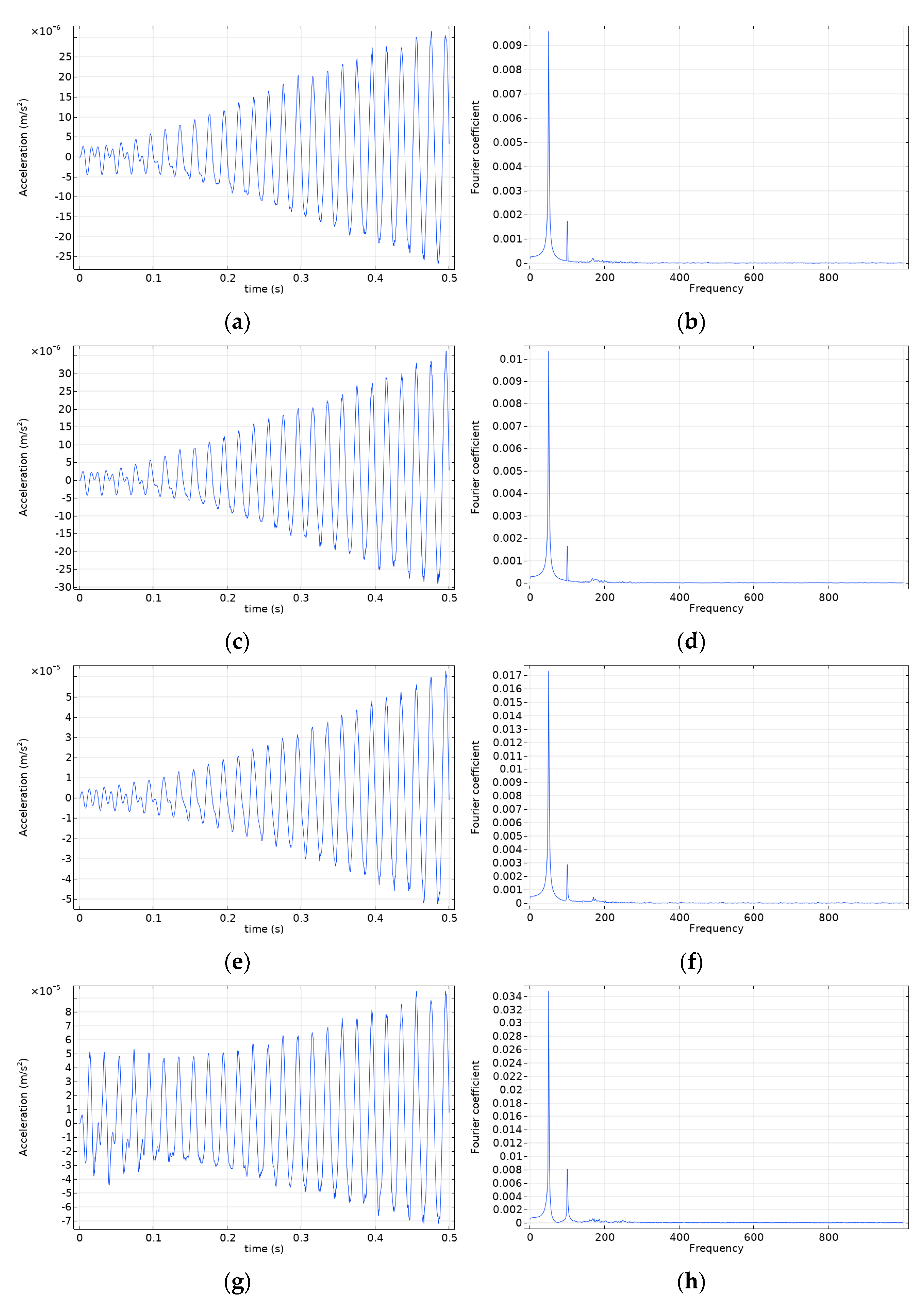
4.2. Analysis of the Vibration Situation under the Transformer Inter–Turn Fault

The degree of vibration in the transformer winding during the interturn discharge that leads to an interturn short circuit will increase when an interturn fault occurs in a transformer. Therefore, the vibration at each point of the transformer can be observed to determine the transformer interturn fault situation [22]. In the 3D model of the transformer, the core point as well as the enclosure point of the transformer will be selected in this paper to study the vibration of the transformer during the whole process. The selected core point and transformer enclosure point are shown in Figure 8, and the vibration of the core point and transformer enclosure point are shown in Figure 9 and Figure 10.
Figure 9 shows that the vibration at the transformer’s core point is pretty regular when the equivalent resistance is 1   Ω . The maximum amplitude of the vibration at the core point is 5 × 10 5   m / s 2 . As the equivalent resistance decreases, the vibration at the core point becomes more and more violent, and the amplitude of the vibration signal becomes larger and larger. When the equivalent resistance is 0.01   Ω , the core point of the transformer will vibrate violently in the first 0.1s when an interturn short circuit occurs. The difference from the previous core point vibration is large, and the maximum amplitude of the core point vibration is 25 × 10 5   m / s 2 . From the spectrum of the core point in Figure 9, it can be seen that the acceleration spectrum of the vibration of the core point is mainly concentrated in the first 500 Hz, with the most intense vibration at 50 Hz and 100 Hz. The spectrum at 50 Hz is mainly due to the three–phase unbalance of the transformer. The majority of the vibration signals in the spectrum at 100 Hz have a fundamental frequency that is two times the frequency of the power supply. The spectrum is mostly made at 100 Hz by a vibration signal with a fundamental frequency that is twice the frequency of the power supply. The spectrum in the 200 ~ 500   Hz range is mainly due to the magnetostriction of the core and the winding inter–turn electrodynamic force. As the equivalent resistance decreases, the vibration of the core point increases, and the Fourier coefficients at the different components increase significantly with the decrease of the equivalent resistance [14].
It can be seen from Figure 10 that the amplitude of the vibration at the transformer enclosure point has a maximum value of 30 × 10 6   m / s 2 when the equivalent resistance is 1   Ω . When the equivalent resistance is 0.01   Ω , the maximum amplitude of the vibration at the transformer enclosure point is 9 × 10 5   m / s 2 . The vibration acceleration spectrum of the transformer enclosure point is still mainly distributed at 50 Hz and 100 Hz, and there will be interharmonics of small amplitude in 200 ~ 500   Hz . As the equivalent resistance decreases, the transformer enclosure point vibration increases. The Fourier coefficients at 50 Hz and 100 Hz increase significantly as the equivalent resistance decreases. However, there is no significant change in the Fourier level of the range. However, there is no significant change in the Fourier magnitude in the range of 200∼500 Hz [23].
It can be concluded that as the transformer inter–turn insulation material ages, the vibration of the transformer core and enclosure points becomes increasingly violent, and the amplitude of the waveform increases. However, the variation of interharmonics at the transformer enclosure point is not as pronounced as at the core point. Thus, the vibration at two points can be used to determine the fault condition of a transformer and to figure out how bad an interturn fault is.

5. Conclusions

In this paper, a three–phase transformer of 10 KV is used as an example. The model is simulated in a transient manner using the finite element method and the field–circuit coupling method. The electromagnetic and mechanical characteristics of the faulty winding during the transformer interturn discharge to the interturn short circuit are comprehensively analyzed. The following conclusions are obtained as a result.
  • In this model, the transformer interturn fault current becomes rapidly larger as the interturn insulation material ages. The magnetic flux density of the core is locally saturated where the fault is. As a result, the short–circuit winding’s local leakage magnetic field expands. When the interturn insulation material is completely damaged, the transformer experiences an interturn short circuit. The winding short–circuit current is tens of times the normal current. The leakage field from the short–circuit fault makes the core vibrate more by locally filling up the magnetic field of the core.
  • When the transformer develops from interturn discharge to interturn short circuit, the strain on the short–circuit winding increases dramatically, resulting in a larger deformation of the short–circuit winding. Finally, the short–circuit winding causes damage. The mechanical characteristics of the winding will be reduced after the deformation occurs, leading to a decrease in short circuit resistance.
  • In the time domain, the amplitude of the waveform at the core and case points increases as the inter–turn insulation material ages. The interharmonic Fourier coefficients also increase in the frequency domain. Therefore, in transformer fault detection, the vibration characteristics of the shell points in the time and frequency domains can be combined to analyze and detect transformer faults.

Author Contributions

Methodology, L.R.; Software, N.Z. and L.Z.; Validation, H.L.; Investigation, L.S. and L.R.; Resources, J.L. and L.R.; Data curation, J.L.; Writing—review & editing, N.Z.; Visualization, N.Z.; Supervision, H.L.; Project administration, L.R.; Funding acquisition, L.Z. All authors have read and agreed to the published version of the manuscript.

Funding

This research was funded by the National Natural Science Foundation of China, grant number 52277016.

Data Availability Statement

The data of the simulation is unavailable because of the privacy issue of the data.

Conflicts of Interest

The authors declare no conflict of interest.

References

  1. Baravati, P.R.; Moazzami, M.; Hosseini, S.M.H.; Mirzaei, H.R.; Fani, B. Achieving the exact equivalent circuit of a large-scale transformer winding using an improved detailed model for partial discharge study. Int. J. Electr. Power Energy Syst. 2022, 134, 107451. [Google Scholar] [CrossRef]
  2. Am, A.; Mv, A.; Ah, B.; Mf, A. HTS transformers leakage flux and short circuit force mitigation through optimal design of auxiliary windings. Cryogenics 2020, 110, 103148. [Google Scholar]
  3. Moradnouri, A.; Vakilian, M.; Hekmati, A.; Fardmanesh, M. Multi-segment Winding Application for Axial Short Circuit Force Reduction Under Tap Changer Operation in HTS Transformers. J. Supercond. Nov. Magn. 2019, 32, 3171–3182. [Google Scholar] [CrossRef]
  4. Moradnouri, A.; Vakilian, M.; Hekmati, A.; Fardmanesh, M. Inductance Calculation of HTS Transformers with Multi-segment Windings Considering Insulation Constraints. J. Supercond. Nov. Magn. 2021, 34, 1–11. [Google Scholar] [CrossRef]
  5. Mikhak-Beyranvand, M.; Faiz, J.; Rezaei-Zare, A.; Rezaeealam, B. Electromagnetic and thermal behavior of a single-phase transformer during Ferroresonance considering hysteresis model of core. Int. J. Electr. Power Energy Syst. 2020, 121, 106078. [Google Scholar] [CrossRef]
  6. Behjat, V.; Vahedi, A. Analysis of internal winding short circuit faults in power transformers using transient finite element method coupling with external circuit equations. Int. J. Numer. Model. Electron. Netw. Devices Fields 2013, 26, 425–442. [Google Scholar] [CrossRef]
  7. Yang, C.; Ding, Y.; Qiu, H.; Xiong, B. Analysis of Turn-to-Turn Fault on Split-Winding Transformer Using Coupled Field-Circuit Approach. Processes 2021, 9, 1314. [Google Scholar] [CrossRef]
  8. Asadi, N.; Kelk, H.M. Modeling, Analysis, and Detection of Internal Winding Faults in Power Transformers. IEEE Trans. Power Deliv. 2015, 30, 2419–2426. [Google Scholar] [CrossRef]
  9. Soleimani, M.; Faiz, J.; Nasab, P.S.; Moallem, M. Temperature Measuring-Based Decision-Making Prognostic Approach in Electric Power Transformers Winding Failures. IEEE Trans. Instrum. Meas. 2020, 69, 6995–7003. [Google Scholar] [CrossRef]
  10. Wang, H.; Butler, K.L. Modeling transformers with internal incipient faults. IEEE Power Eng. Rev. 2007, 22, 64. [Google Scholar] [CrossRef]
  11. Etumi, A.A.A.; Anayi, F.J. The Application of Correlation Technique in Detecting Internal and External Faults in Three-Phase Transformer and Saturation of Current Transformer. IEEE Trans. Power Deliv. 2016, 31, 2131–2139. [Google Scholar] [CrossRef]
  12. Oliveira, L.M.R.; Cardoso, A.J.M. A Permeance-Based Transformer Model and Its Application to Winding Interturn Arcing Fault Studies. IEEE Trans. Power Deliv. 2010, 25, 1589–1598. [Google Scholar] [CrossRef] [Green Version]
  13. Zhang, C.; Ge, W.; Xie, Y.; Li, Y. Comprehensive Analysis of Winding Electromagnetic Force and Deformation During No-Load Closing and Short-Circuiting of Power Transformers. IEEE Access 2021, 9, 73335–73345. [Google Scholar] [CrossRef]
  14. Duan, X.; Zhao, T.; Liu, J.; Zhang, L.; Zou, L. Analysis of Winding Vibration Characteristics of Power Transformers Based on the Finite-Element Method. Energies 2018, 11, 2404. [Google Scholar] [CrossRef] [Green Version]
  15. Zhang, H.; Yang, B.; Xu, W.; Wang, S.; Wang, G.; Huangfu, Y.; Zhang, J. Dynamic Deformation Analysis of Power Transformer Windings in Short-Circuit Fault by FEM. IEEE Trans. Appl. Supercond. 2014, 24, 1–4. [Google Scholar] [CrossRef]
  16. Jia, X.; Lin, M.; Su, S.; Wang, Q.; Yang, J. Numerical study on temperature rise and mechanical properties of winding in oil-immersed transformer. Energy 2022, 239, 121788. [Google Scholar] [CrossRef]
  17. Behjat, V.; Vahedi, A. An experimental approach for investigating low-level interturn winding faults in power transformers. Electr. Eng. 2013, 95, 135–145. [Google Scholar] [CrossRef]
  18. Nia, M.S.S.; Shamsi, P.; Ferdowsi, M. Investigation of Various Transformer Topologies for HF Isolation Applications. IEEE Trans. Plasma Sci. 2020, 48, 512–521. [Google Scholar]
  19. Li, M.; Wang, Z.; Zhang, J.; Ni, Z.; Tan, R. Temperature Rise Test and Thermal-Fluid Coupling Simulation of an Oil-Immersed Autotransformer Under DC Bias. IEEE Access 2021, 9, 32835–32844. [Google Scholar] [CrossRef]
  20. Liu, X.; Yang, Y.; Huang, Y.; Jadoon, A. Vibration characteristic investigation on distribution transformer influenced by DC magnetic bias based on motion transmission model. Int. J. Electr. Power Energy Syst. 2018, 98, 389–398. [Google Scholar] [CrossRef]
  21. Wang, S.; Zhang, H.; Wang, S.; Li, H.; Yuan, D. Cumulative Deformation Analysis for Transformer Winding Under Short-Circuit Fault Using Magnetic–Structural Coupling Model. IEEE Trans. Appl. Supercond. 2016, 26, 0606605. [Google Scholar] [CrossRef]
  22. Zhang, F.; Ji, S.; Shi, Y.; Ren, F.; Zhan, C.; Zhu, L. Comprehensive vibration generation model of transformer winding under load current. IET Gener. Transm. Distrib. 2019, 13, 1563–1571. [Google Scholar] [CrossRef]
  23. Jingzhu, H.; Dichen, L.; Qingfen, L.; Yang, Y.; Shanshan, L. Electromagnetic vibration noise analysis of transformer windings and core. IET Electr. Power Appl. 2016, 10, 251–257. [Google Scholar] [CrossRef]
Figure 1. Parallel Equivalent circuit of a dielectric material.
Energies 16 00512 g001
Figure 2. Simulation circuit.
Energies 16 00512 g002
Figure 3. 3–D model of power transformer.
Energies 16 00512 g003
Figure 4. The currents of primary and secondary side under fault conditions; they should be listed as: (a) Primary side current of R eq = 1   Ω ; (b) Secondary side current of R eq = 1   Ω ; (c) Primary side current of R eq = 0.5   Ω ; (d) Secondary side current of R eq = 0.5   Ω ; (e) Primary side current of R eq = 0.1   Ω ; (f) Secondary side current of R eq = 0.1   Ω ; (g) Primary side current of R eq = 0.01   Ω ; (h) Secondary side current of R eq = 0.01   Ω .
Energies 16 00512 g004
Figure 5. The currents of primary and secondary side under normal conditions.
Energies 16 00512 g005
Figure 6. The distribution of transformer magnetic field under interturn fault, which should be listed as: (a) The distribution of magnetic field of R eq = 1   Ω ; (b) The distribution of magnetic field of R eq = 0.5   Ω ; (c) The distribution of magnetic field of R eq = 0.1   Ω ; (d) The distribution of magnetic field of R eq = 0.01   Ω .
Energies 16 00512 g006
Figure 7. Transformer strain and displacement distribution under fault conditions, which should be listed as: (a) Strain distribution of R eq = 1   Ω ; (b) Displacement distribution of R eq = 1   Ω ; (c) Strain distribution of R eq = 0.5   Ω ; (d) Displacement distribution of R eq = 0.5   Ω ; (e) Strain distribution of R eq = 0.1   Ω ; (f) Displacement distribution of R eq = 0.1   Ω ; (g) Strain distribution of R eq = 0.01   Ω ; (h) Displacement distribution of R eq = 0.01   Ω .
Energies 16 00512 g007aEnergies 16 00512 g007b
Figure 8. The location of the transformer observation point; they should be listed as: (a) The position of the core point; and (b) The position of the transformer enclosure point.
Energies 16 00512 g008
Figure 9. The vibration and spectrum diagram of transformer core point, they should be listed as: (a) Core point vibration of R eq = 1   Ω ; (b) Core point spectrum of R eq = 1   Ω ; (c) Core point vibration of R eq = 0.5   Ω ; (d) Core point spectrum of R eq = 0.5   Ω ; (e) Core point vibration of R eq = 0.1   Ω ; (f) Core point spectrum of R eq = 0.1   Ω ; (g) Core point vibration of R eq = 0.01   Ω ; (h) Core point spectrum of R eq = 0.01   Ω .
Energies 16 00512 g009aEnergies 16 00512 g009b
Figure 10. The vibration and spectrum diagram of the transformer enclosure point; they should be listed as: (a) Enclosure point vibration of R eq = 1   Ω ; (b) Enclosure point spectrum of R eq = 1   Ω ; (c) Enclosure point vibration of R eq = 0.5   Ω ; (d) Enclosure point spectrum of R eq = 0.5   Ω ; (e) Enclosure point vibration of R eq = 0.1   Ω ; (f) Enclosure point spectrum of R eq = 0.1   Ω ; (g) Enclosure point vibration of R eq = 0.01   Ω ; (h) Enclosure point spectrum of R eq = 0.01   Ω .
Energies 16 00512 g010
Table 1. Parameters of transformer.
Main Technical IndicatorsParameter
Phase numberthree–phase
Rated frequency50 Hz
Rated capacity/kVA100
Rated voltage/kV10/0.4
Linkage group numberYyn0
short–circuit impedance (%)4.0
Table 2. Parameters of transformer winding and core.
Main Technical IndicatorsParameter
Number of turns of high voltage winding500
Number of turns of low voltage winding20
Diameter of high voltage winding/cm22–23
Diameter of low voltage winding/cm23–24
Height of high voltage winding/cm50
Height of low voltage winding/cm50
Shell size(W×H×D)/cm250 × 150 × 100
Height of the upper and lower yoke of the core/cm102.4
Core thickness/cm20
Core length/cm128.48
Core column radius of core/cm21
Disclaimer/Publisher’s Note: The statements, opinions and data contained in all publications are solely those of the individual author(s) and contributor(s) and not of MDPI and/or the editor(s). MDPI and/or the editor(s) disclaim responsibility for any injury to people or property resulting from any ideas, methods, instructions or products referred to in the content.

