Abstract
Due to the increasing penetration of the power grid with renewable, distributed energy resources, new strategies for voltage stabilization in low voltage distribution grids must be developed. One approach to autonomous voltage control is to apply reinforcement learning (RL) for reactive power injection by converters. In this work, to implement a secure test environment including real hardware influences for such intelligent algorithms, a power hardware-in-the-loop (PHIL) approach is used to combine a virtually simulated grid with real hardware devices to emulate as realistic grid states as possible. The PHIL environment is validated through the identification of system limits and analysis of deviations to a software model of the test grid. Finally, an adaptive volt–var control algorithm using RL is implemented to control reactive power injection of a real converter within the test environment. Despite facing more difficult conditions in the hardware than in the software environment, the algorithm is successfully integrated to control the voltage at a grid connection point in a low voltage grid. Thus, the proposed study underlines the potential to use RL in the voltage stabilization of future power grids.
1. Introduction
As part of the energy transition process in Germany, the government’s goal is to increase the share of renewable energies in gross power consumption from 45.5% (2020) to at least 80% [1]. In order to achieve this, both an increase in renewable generation capacity and a reduction in the number of conventional power plants are being realized. This leads to a low voltage distribution grid which is dominated by power converters in the future. These changes entail new requirements in the power grid operation and especially in the provision of ancillary services [2].
In this regard, there are standardized reactive power control strategies currently used for static voltage control, which are rather inflexible [3,4]. This means that they are not adaptable to the individual grid characteristics at different grid connection points (GCPs). Thus, there is a high potential to advance current approaches or to replace them with a GCP-specific reactive power management [5]. An advantage of using such advanced methods to provide reactive power by converter systems would be to counteract the grid expansion as the grid capacities could be exploited more efficiently. This means that new generations of power plants on a larger scale could be installed at the nearest grid connection point [6]. Thus, unnecessary losses of electricity caused by the increased length of connection cables would be avoided. Accordingly, the current state of the art indicates that there is a large interest in grid-supporting reactive power management.
In this context, for example, Sun et al. and Chamana et al. developed new methods to deal with optimal local power control for photovoltaic inverters in active distribution grids using convolutional neural networks [7,8].
Another concept, which becomes interesting in the context of reactive power control, is reinforcement learning (RL). RL is a state-of-the-art research field that is attracting attention in many application areas, especially in gaming and robotics [9,10]. It is also becoming increasingly significant in the field of power and energy applications. Thus, Perera et al. deal with the evaluation of RL applications in energy systems [11]. For this purpose, they classified RL publications into different categories based on their scope of application.
Concerning the approach for reactive power control, there are several studies using RL, e.g., by Wang et al. who examined an approach based on a soft actor critical algorithm [12]. Other RL-based investigations can be found, e.g., by Fan et al., Liu et al., Gao et al., and Zhang et al. [13,14,15,16]. However, all these algorithms were developed and purely tested within simulative models. In order to apply such approaches in future real-power grids, a hardware-based validation of these algorithms is required in addition to the simulative validation.
An often-used methodology to combine physical and simulative components is the power hardware-in-the-loop (PHIL) approach. This framework was used, e.g., by Roscoe et al. who developed an environment in which a laboratory grid topology consisting of generators, loads, controls, protection devices, and switches can be simulated [17]. Next to this, Ebe et al. and Hoke et al. tested commercial devices and their control strategies in a PHIL environment [18,19]. Furthermore, Kotsampopoulos et al. presented a benchmark system for hardware-in-the-loop testing of distributed energy resources [20].
Within the scope of this study, the reactive power management approach using RL in converters by Beyer et al., which is another purely simulative investigation of a deep deterministic policy gradient (DDPG) algorithm [21], will be implemented in a hardware environment. To this end, a PHIL setup is developed, which allows for the combination of physical power components with a power grid simulated in real-time and finally for the validation of a RL-based reactive power control algorithm.
This leads to the following main contributions of this study:
- In this study, a hardware-based test environment emulating a low voltage distribution grid is implemented and validated. This setup enables the testing of machine learning algorithms while facing the influences of real hardware components.
- A reinforcement learning agent is successfully used to stabilize the grid voltage by controlling reactive power injection within the hardware-based environment. The performance is investigated in comparison to a software setup. By this, the results of a purely simulative study can be confirmed in a hardware context.
This paper is organized as follows. At the beginning, the concept of this work is introduced in Section 2. Based on this, the implementation of a PHIL environment for training and testing a machine learning algorithm is presented, and the integration of the control algorithm into this environment is described. Section 3 illustrates the performance of the algorithm in this hardware environment and compares the results with a software-based environment approach. Section 4 concludes this paper with a summary and an outlook on possible further developments of this work.
2. Materials and Methods
With the future goal to apply a RL-based reactive power management algorithm in real converter systems, it is required to implement it into a real converter control as well as to adapt the training and validation environment through integration of real hardware components. Furthermore, a communication strategy between the environment, the external algorithm, and the internal active and reactive power control of a converter has to be developed. Thereby, the overall goal is to stabilize the grid voltage in a low voltage grid.
During the course of this work, the voltage values are normalized to the nominal voltage (400 V) and denoted in per unit (pu) specification.
In this section, the general methodology to test a RL algorithm for reactive power control within a hardware-based test environment is presented.
The applied concept of RL is based on two fundamental components: the agent and the environment. The general principle of reinforcement learning is that in each step the agent gets the current state of the environment and selects an action based on this. By this action, the environment is changed to a new state. Based on this new state and a predefined learning goal, the agent receives a reward signal, which is used to adjust the behavior of the agent and to select a new action. The following section deals with the environment needed for RL.
2.1. Test Environment
To test the RL control algorithm in voltage control of a low voltage distribution grid, the first step of this study was to build up an appropriate environment in the grid lab NESTEC of the DLR institute [22]. In this section, the implementation of this setup and the concept to test the algorithm are described.
From a higher perspective, the setup consisted, on the one hand, of a software-based part to simulate a power grid and, on the other hand, of some hardware components to emulate parts of the considered grid in reality. To connect both sides of this setup, a PHIL approach was used, and finally, a reactive power control was implemented at a particular GCP, which was emulated in hardware.
Overall, the PHIL setup is composed of a Speedgoat real-time system and two power amplifiers as the PHIL’s power hardware devices, one to emulate a grid and one to implement a control algorithm. In Figure 1, the setup is shown in detail.
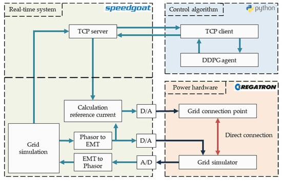
Figure 1.
Integration of the DDPG agent into the PHIL environment (red: power exchange, blue: digital signal, black: analog signal).
On the grid simulation side, the three-phase reference grid no. 8 for low voltage distribution grids from the MONA 2030 project [23] was modeled in MATLAB/Simulink (release 2020b) using the toolboxes Simscape and Simscape Electrical [24,25]. Therefore, the grid model contained a low voltage grid of 0.4 kV including ten GCPs and a transformer that connects to a virtual medium voltage level of 11 kV. Between transformer and load busses, several power grid lines were implemented to represent real cable conditions of different types and lengths. As indicated in Figure 1, the model was executed with a step size of 100 µs on a Speedgoat real-time system, which represented the interface to the hardware [26]. Furthermore, the power grid was viewed from the perspective of generation plants [27].
Following a hybrid approach by Muhammad et al. based on the concept of Plumier et al. [28,29], the grid simulation was set to run in phasor mode, which allows it to simulate large power grids without over-loading the computational capacities of the real-time system. In addition, a conversion from phasor to EMT domain was included to transform phasor values into discrete sinusoidal signals of voltage and current.
On the hardware side of the setup, the idea was to represent a single grid connection point in hardware where a converter is controlled by a RL algorithm in order to stabilize the grid voltage. For this, it was necessary to emulate the simulated grid voltage with hardware and also to integrate a converter which can be externally controlled (see Figure 1, grid simulator and grid connection point).
These components were represented by two 30 kVA, 4-quadrant amplifiers of type TopCon TC.ACS from the manufacturer Regatron AG [30], which were connected in series. Both converters were configured to run in amplifier mode. This means that they receive reference signals, which are amplified by the device. To that end, the signals from EMT domain in the Simulink model were down-scaled to ranges of −10 to 10 V and afterwards transmitted to the hardware components via field-programmable gate arrays (FPGAs) as analog signals.
In this way, the first amplifier was used to emulate the grid voltage. For the external control of the second one for reactive power management, a TCP server was integrated in the Simulink model. This server represented the interface to exchange data between the real-time system and the control algorithm connected to a TCP client in Python. In detail, the mean voltage of the three grid phases and setpoints for reactive power control by the second amplifier were exchanged using the TCP server, which was running with a step size of 0.5 s in parallel to the grid simulation and reference signal generation.
2.2. Control Algorithm
In this section, the control algorithm and its application are proposed. As mentioned in the previous sections, the algorithm used in this study belongs to the class of RL. More precisely, the presented investigations were conducted using the deep reinforcement learning approach by Beyer et al. and their optimized agent parameters and inputs [21]. This approach is based on the DDPG, which was developed by Lillicrap et al. as a model-free actor-critic method [31]. This means that the architecture of the algorithm separates the learning process into two distinct parts: the actor, which determines the next action to take based on the current state of the environment, and the critic, which evaluates the action taken by the actor and provides feedback to improve the actor’s decision-making. The DDPG is particularly useful for learning policies in continuous action spaces. One special property of the DDPG algorithm is that it uses a deterministic policy, which means that the actor’s part of the algorithm always outputs the same action for a given state. This simplifies the learning process and allows the algorithm to converge to a solution faster than other reinforcement learning algorithms that use stochastic policies [31].
The RL framework was implemented in Python using the libraries OpenAIGym and keras-rl to build the RL cycle shown in Figure 2 [32,33].
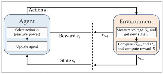
Figure 2.
Interaction between agent and environment in reinforcement learning, according to [34]. The learning goal is to maintain the measured voltage (Um) close to nominal value (Unom) of 1 pu.
In this study, the DDPG agent was required to stabilize the grid voltage. Therefore, as indicated in Figure 2, in the test environment from Section 2.1, the voltage Um was necessarily measured. Based on this, the environment’s state was determined. The state consisted of the difference to the nominal voltage of 1 pu, the real and imaginary parts, and the derivation of the voltage (see Equation (1)).
In addition, the measured (Um) and the nominal voltage (Unom = 1 pu) were compared, and a reward signal was computed as:
With this reward function, the learning objective was set to keep the voltage inside a tolerance band of ±0.005 pu. The first term evaluated the deviation from the ideal voltage, while the second term rewarded longer periods of time when the voltage was kept within a specified tolerance band, since it is not possible to achieve a constant voltage value under real hardware influences. As the test environment contained a very stable power grid, there were no large voltage changes observable. The voltage tolerance band of ±10% of real power grids has not been violated by possible load changes within a stable test environment (see Table 1). For these two reasons, the interval of ±0.005 pu was considered in the reward function.

Table 1.
Stability analysis—Limits of active and reactive power for stable system operation.
Both state and reward signals were transmitted to the agent. As the next step in Figure 2, the agent’s action policy was adjusted by updating the weights of the internal neural networks of the actor and critic. After that, the agent selected an action. In this study, this represented the setpoint for the reactive power to be injected by the converter. Following this setpoint, the grid voltage in the test environment was affected, and the agent’s environment changed to a new state.
3. Results and Discussion
This section deals with the validation of the hardware-based test environment described in Section 2.1 and presents the results of the application of a RL agent in reactive power control inside the developed hardware environment.
3.1. Validation of the Hardware Environment in Terms of Stability and Deviation from the Software Model
In this section, the differences between the software and the hardware environments are examined, considering that there are often discrepancies in the results when transferring from a simulated model to a real environment [35]. These deviations may be caused by noise, or other undesirable interactions between hardware components may occur.
The hardware setup’s stability limits were identified based on a harmonic analysis. For this, the system was considered as stable until the share of the 9th harmonic significantly increases. To find the limits, a stepwise increase and decrease in active and reactive power was separately performed, while the other quantity was set to zero. As a result, the limit values shown in Table 1 were obtained.
As a result, the test environment can be operated in a stable manner within the limits shown in Table 1. This means that a RL algorithm can be safely trained and tested as long as the corresponding actions and power values are chosen under consideration of these limits.
In addition to the stability, the deviation of the test setup to a comparable software-based environment was investigated. The ideal characteristic curves of reactive power as a function of active power (Q(P)) in the PHIL environment and in the simulative environment were determined and compared with each other.
Figure 3 shows the contour lines for active and reactive power tuples resulting in the nominal voltage, i.e., U(P, Q) = 1 pu, for the virtual test grid (blue) and for the PHIL environment (orange).
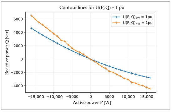
Figure 3.
Contour lines representing tuples of reactive power (Q) and active power (P) leading to nominal voltage in software (SW, blue line) and hardware (HW, orange line).
The contour line values were determined by increasing the active power at the selected GCP from −16 kW to 16 kW in 1 kW increments and determining the associated reactive power value that decreases or increases the voltage to 1 pu.
Both resulting contour lines are slightly curved, but with different degrees of curvature. More precisely, to achieve a voltage value of 1 pu in the software environment, there was a need for reactive power in a range of −3 to 4.6 kvar. The same goal was reached in the hardware environment with a reactive power in an interval of −4.5 to 6.5 kvar. Thus, in the considered power ranges in the hardware environment, approximately 50% more reactive power was required to achieve the ideal voltage value.
It is assumed that the difference is caused by the capacitors used in the power amplifier. These capacitors act as low-pass filters for the output and cause the device to operate as a capacitive-resistive load instead of a resistive load as expected.
In addition, the delay of voltage changes in consequence of active power changes was analyzed in both environments. An example of this analysis is shown in Figure 4.
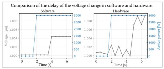
Figure 4.
Comparison of the delay of the voltage change in software and hardware when changing the active power.
For the investigation of the delay, the power grid in the test environment was simulated without any voltage control algorithm. During the simulation, the randomly chosen active power values were transmitted to the power amplifier, and the voltage was measured in parallel. As shown in Figure 4, in the example of the transition from 0 kW to 3 kW, there is a delay between the change of voltage and the adaption of active power in both software and hardware environments.
Here, the new active power value was set after three steps. The graph reveals that the voltage in the software environment increased to about 1.004 pu after a delay of five steps. In the hardware environment, this increase happened after seven steps.
Further analysis showed that this behavior is present for any size of active power change and throughout the entire time of simulation.
Moreover, it is interesting to note that the graphs show a different voltage reaction to the same amount of active power. In the software environment, no voltage band (±0.005 pu) violation occurred when the active power was set to 3 kW. This is different in the hardware where the voltage rose above 1.006 pu, such that the tolerance band was exceeded without injecting reactive power.
Thus, the task of voltage control is more difficult in a hardware than in a software environment.
Subsequently, the RL-based control algorithm (see Section 2.2) was integrated into both environments (software and hardware). The obtained results during the training and test run are discussed in the following section.
Thereby, the agent trained and tested in the simulation is designated as SW-agent, and the one applied in the hardware environment is referred to as HW-agent.
3.2. Training
In training, the agent was first trained in both environments, software and hardware, over a period of 20,000 steps with a TCP server clock of 0.5 s, which corresponds to a time of 10,000 s.
During training, the amplifier emulating the grid connection point was required to inject a certain amount of active power, which was randomly selected in the Python script every 50 s in an interval from 0 to 8 kW in 1 kW steps. The active power values were symmetrically distributed to the three phases of the grid. These active power values were transmitted to the TCP server in the Simulink model every 0.5 s along with the agent’s action, i.e., the reactive power.
The agent was allowed to choose a new action every two timesteps, i.e., every second, based on its observation. The observation was represented by the mean of the three-phase voltage values in per unit specification.
This procedure led to the following training results.
Figure 5 shows the reward of the agents in the training run in software (SW) and hardware (HW) averaged over time. As expected due to fewer disturbances in the simulation environment, the reward curve for the SW-agent lies above the curve for the HW-agent. However, the reward of both agents apparently increases until the end of training, which indicates that both agents were still learning, and a longer training duration could improve the results.
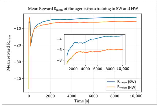
Figure 5.
Mean reward Rmean of the agents increasing throughout training in software (SW) and hardware (HW).
3.3. Test Run
For the test run, the trained agent from the previous section was used in the software and hardware environments to examine its learned behavior. For this, a test period of 4000 steps was set in Python.
Figure 6 displays a part of the test run for both SW- and HW-agent. In detail, sections of the voltage curves from both environments are shown (Figure 6a,b) as well as the associated active and reactive power curves (Figure 6c,d). The active power was regularly changed in a range of 4 to 7 kW. Every time the active power feed-in changes, a voltage peak occurs in both graphs. This behavior might be explained by the delay between the change in active power and the change of the voltage, resulting in a delay in adjusting the reactive power. Furthermore, in the hardware environment, the agent faced a more fluctuating voltage due to hardware influences and measurement inaccuracies. Therefore, the reaction of the agent is less constant than in the software environment, as shown in the reactive power curve of Figure 6d.
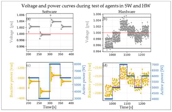
Figure 6.
Sections of voltage curves corresponding to agent in software (SW) (a) and hardware (HW) (b) environments with associated active and reactive power values in SW (c) and HW (d) during the test run.
Despite these differences, it can be seen that both agents were able to keep the voltage inside the defined tolerance band during the presented part of the test.
For a comparison of the total performance, the Q(P) values obtained during the whole test run are shown in Figure 7.
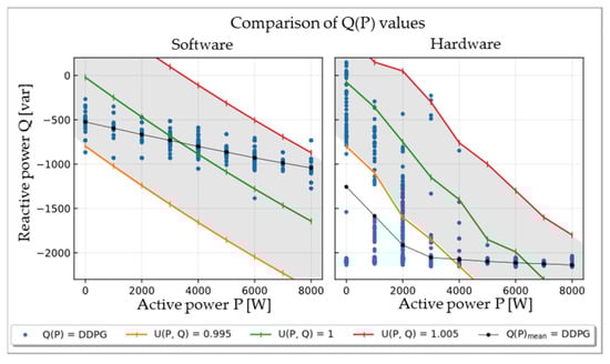
Figure 7.
Comparison of Q(P) values of the trained agents from software and hardware in the test run under consideration of the Q(P) contour lines associated with the tolerance band limits of ±0.005 pu.
In Figure 7, the green curve represents the previously determined contour line to achieve ideal voltage of 1 pu. Similarly, the red and orange curves represent the contour lines of 1 ± 0.005 pu as limits of the set tolerance band. Thus, those curves mark the desired area for Q(P) values returned by the agents (gray).
It can be noticed that all values yielded by the SW-agent are located in this area. In contrast, the results from the HW-agent were more fluctuating, and the limits were crossed, especially for low active power values. As the voltage in the hardware environment itself is far more fluctuating, the strong scattering behavior was expected. Thus, the violations of the tolerance band limits might be explained by the resulting delay explained below Figure 6. Nevertheless, the average curve, which consists of the mean of the Q(P) values for each active power value, is close to the targeted range. Under consideration of the still increasing reward at the end of training, it can be suspected that the agent’s behavior would become even more successful by extending the training time. Thus, further approximation of the targeted range can be expected.
4. Conclusions
This paper presented the implementation of a RL-based algorithm for individualized reactive power provision at a certain GCP in low-voltage grids into a real hardware environment and the validation of its effectiveness in a test environment. An approach was taken to build a PHIL environment that allows for the training and validation of machine learning algorithms in real-time. This involved transferring a GCP from the simulated MONA-8 reference grid into hardware.
Within this environment, a previously developed RL approach based on the DDPG algorithm was used to stabilize the grid voltage. Thereby, reactive power setpoints were computed and transmitted to the internal control of a real hardware component, a four-quadrant amplifier, to inject reactive power into the physically built test grid.
Before using the RL algorithm for voltage control, the system’s stability limits were determined, and the differences between the software and hardware environments were investigated. Based on this comparison, it was found that up to 50%, i.e., −3 kvar in SW and −4.5 kvar in HW (see Section 3.1), more reactive power had to be specified in the hardware environment compared to the software environment. Additional difficulties for the agent in the hardware were measurement inaccuracies and the typical noise of a power grid.
This investigation emphasized the importance to validate RL algorithms in hardware-based environment as the challenges the HW-agent faced are apparently different to simulation models. In a well-defined PHIL setup, realistic behavior of loads at various GCPs from different low-voltage grid topologies can be emulated.
Due to the usage of real power amplifiers and the resulting effect on grid impedance in the test grid, the simulatively developed DDPG algorithm was adapted for application within the proposed PHIL environment. As shown in Section 3.2 and Section 3.3, the algorithm was able to solve the control task in principle in both the software and hardware environments. In some grid situations, the algorithm showed weaknesses due to hardware influences and delay times. However, it was proven that it is possible to train a RL agent in hardware such that it can adapt reactive power injection to stabilize the voltage.
To improve the control results, the algorithm could be further trained or optimized to approximate the ideal reactive power setpoints, e.g., through modification of the reward function or optimization of algorithm parameters. Next to this, further development of the test environment would be conceivable to reduce the delay times for voltage changes as they were apparent in Figure 6. In addition, the Simulink model and the control of the hardware components could be optimized in terms of the reaction times and the resulting voltage changes.
Future work using the proposed setup could deal with the behavior of the agent in more complex grid situations with more active grid participants or after emulating larger parts of the test grid into hardware based on a concept presented by Ahmed et al. [36]. Especially under more complex grid conditions, the agent’s performance could be improved through longer training periods or through provision of more information about the actual grid, for example by integrating the load recognition algorithm by Schlachter et al. [37]. Other interesting studies could address the parallel operation of multiple agents and their interaction.
Finally, it can be stated that the proposed study showed a successful approach to implement a RL-based reactive power control algorithm into a real converter control within a hardware-based environment to validate and test in realistic grid scenarios. These promising results open up many further possibilities for industry-oriented research in view of intelligent and self-learning converters to stabilize and optimally use the capacities of future power grids without external control.
Author Contributions
Conceptualization, O.B., H.S., V.B. and S.G.; methodology, O.B., H.S. and V.B.; software, O.B.; validation, O.B., H.S. and V.B.; formal analysis, O.B.; investigation, O.B.; resources, O.B.; data curation, O.B.; writing—original draft preparation, O.B., H.S. and V.B.; writing—review and editing, S.G.; visualization, O.B. and H.S.; supervision, S.G. and K.v.M.; project administration, V.B.; funding acquisition, S.G. and K.v.M. All authors have read and agreed to the published version of the manuscript.
Funding
This research belongs to the research project SiNED and is funded by the Lower Saxony Ministry of Science and Culture (Niedersächsisches Ministerium für Wissenschaft und Kultur) through the “Niedersächsisches Vorab” grant program, grant number ZN3563, and of the Energy Research Centre of Lower Saxony.
Data Availability Statement
No new data were created or analyzed in this study. Data sharing is not applicable to this article.
Acknowledgments
The research project “SiNED—Systemdienstleistungen für sichere Stromnetze in Zeiten fortschreitender Energiewende und digitaler Transformation” acknowledges the support of the Lower Saxony Ministry of Science and Culture through the “Niedersächsisches Vorab” grant programme (grant ZN3563) and of the Energy Research Centre of Lower Saxony. The authors would also like to thank Moiz Ahmed, Holger Behrends, Thomas Esch, and Gerrit Bremer for their support in the hardware implementation and their advice in electrotechnical aspects of this study.
Conflicts of Interest
The authors declare no conflict of interest.
Abbreviations
The following abbreviations are used in this manuscript:
| DDPG | Deep deterministic policy gradient |
| DLR | German Aerospace Center |
| EMT | Electromagnetic transients |
| FPGA | Field-programmable gate arrays |
| GCP | Grid connection point |
| PHIL | Power hardware-in-the-loop |
| pu | per unit |
| RL | Reinforcement learning |
| TCP | Transmission control protocol |
References
- Erneuerbare-Energien-Gesetz—EEG 2017 in Germany. 2017. Available online: https://www.gesetze-im-internet.de/eeg_2014/EEG_2017.pdf (accessed on 9 August 2022).
- Deutsche Energie-Agentur GmbH (dena). Dena Studie Systemdienstleistungen 2030; Deutsche Energieagentur: Berlin, Germany, 2014; Available online: https://www.dena.de/fileadmin/dena/Dokumente/Pdf/9094_dena-Studie_Systemdienstleistungen_2030.pdf (accessed on 9 August 2022).
- Demirok, E.; González, P.C.; Frederiksen, K.H.B.; Sera, D.; Rodriguez, P.; Teodorescu, R. Local Reactive Power Control Methods for Overvoltage Prevention of Distributed Solar Inverters in Low-Voltage Grids. IEEE J. Photovolt. 2011, 1, 174–182. [Google Scholar] [CrossRef]
- Malekpour, A.R.; Pahwa, A. Reactive power and voltage control in distribution systems with photovoltaic generation. In Proceedings of the North American Power Symposium (NAPS), Champaign, IL, USA, 9–11 September 2012; pp. 1–6. [Google Scholar] [CrossRef]
- Duan, J.; Li, H.; Zhang, X.; Diao, R.; Zhang, B.; Shi, D.; Lu, X.; Wang, Z.; Wang, S. A deep reinforcement learning based approach for optimal active power dispatch. arXiv 2019. [Google Scholar] [CrossRef]
- SMA Solar Technology, AG. SMA verschiebt die Phase. Available online: https://www.sma.de/partner/expertenwissen/sma-verschiebt-die-phase (accessed on 10 August 2022).
- Sun, X.; Qiu, J.; Zhao, J. Optimal local volt/var control for photovoltaic inverters in active distribution networks. IEEE Trans. Power Syst. 2021, 36, 5756–5766. [Google Scholar] [CrossRef]
- Sun, X.; Qiu, J.; Tao, Y.; Ma, Y.; Zhao, J. A multi-mode data-driven volt/var control strategy with conservation voltage reduction in active distribution networks. IEEE Trans. Sustain. Energy 2022, 13, 1073–1085. [Google Scholar] [CrossRef]
- Lu, W.-F.; Yang, J.-K.; Chu, H.-T. Playing mastermind game by using reinforcement learning. In Proceedings of the IEEE International Conference on Robotik Computing (IRC), Taichung, Taiwan, 10–12 April 2017; pp. 418–421. [Google Scholar] [CrossRef]
- Gamble, C.; Gao, J. Safety-first AI for autonomous data centre cooling and industrial control. Available online: https://www.deepmind.com/blog/safety-first-ai-for-autonomous-data-centre-cooling-and-industrial-control (accessed on 10 August 2022).
- Perera, A.T.D.; Kamalaruban, P. Applications of reinforcement learning in energy systems. Renew. Sustain. Energy Rev. 2021, 137, 110618. [Google Scholar] [CrossRef]
- Wang, W.; Yu, N.; Gao, Y.; Shi, J. Safe off-policy deep reinforcement learning algorithm for volt-VAR control in power distribution systems. IEEE Trans. Smart Grid 2020, 11, 3008–3018. [Google Scholar] [CrossRef]
- Fan, T.-H.; Lee, X.Y.; Wang, Y. PowerGym: A reinforcement learning environment for volt-var control in power distribution systems DeepAI 2021. Available online: https://deepai.org/publication/powergym-a-reinforcement-learning-environment-for-volt-var-control-in-power-distribution-systems (accessed on 9 August 2022).
- Liu, H.; Wu, W. Two-stage deep reinforcement learning for inverter-based volt-VAR control in active distribution networks. IEEE Trans. Smart Grid 2021, 12, 2037–2047. [Google Scholar] [CrossRef]
- Gao, Y.; Wang, W.; Yu, N. Consensus multi-agent reinforcement learning for volt-VAR control in power distribution networks. IEEE Trans. Smart Grid 2021, 12, 3594–3604. [Google Scholar] [CrossRef]
- Zhang, Y.; Wang, X.; Wang, J.; Zhang, Y. Deep reinforcement learning based volt-VAR optimization in smart distribution systems. IEEE Trans. Smart Grid 2021, 12, 361–371. [Google Scholar] [CrossRef]
- Roscoe, A.J.; Mackay, A.; Burt, G.M.; McDonald, J.R. Architecture of a network-in-the-loop environment for characterizing AC power-system behavior. IEEE Trans. Ind. Electron. 2009, 57, 1245–1253. [Google Scholar] [CrossRef]
- Ebe, F.; Idlbi, B.; Stakic, D.E.; Chen, S.; Kondzialka, C.; Casel, M.; Heilscher, G.; Seitl, C.; Bründlinger, R.; Strasser, T.I. Comparison of power hardware-in-the-loop approaches for the testing of smart grid controls. Energies 2018, 11, 3381. [Google Scholar] [CrossRef]
- Hoke, A.; Chakraborty, S.; Basso, T. A power hardware-in-the-loop framework for advanced grid-interactive inverter testing. In Proceedings of the IEEE Power & Energy Society Innovative Smart Grid Technologies Conference (ISGT), Washington, DC, USA, 18–20 February 2015; pp. 1–5. [Google Scholar]
- Kotsampopoulos, P.; Lagos, D.; Hatziargyriou, N.; Faruque, M.O.; Lauss, G.; Nzimako, O.; Forsyth, P.; Steurer, M.; Ponci, F.; Monti, A.; et al. A benchmark system for hardware-in-the-loop testing of distributed energy resources. IEEE Power Energy Technol. Syst. 2018, 5, 94–103. [Google Scholar] [CrossRef]
- Beyer, K.; Beckmann, R.; Geißendörfer, S.; von Maydell, K.; Agert, C. Adaptive online-learning volt-var control for smart inverters using deep reinforcement learning. Energies 2021, 14, 1991. [Google Scholar] [CrossRef]
- Deutsches Zentrum für Luft- und Raumfahrt e. V. (DLR). DLR eröffnet Emuationszentrum für Vernetzte Energiesysteme (NESTEC) am Standort Oldenburg. Available online: https://www.dlr.de/content/de/artikel/news/2019/04/20191126_dlr-eroeffnet-emulationszentrum-fuer-vernetzte-energiesysteme-nestec.html (accessed on 10 August 2022).
- Forschungsstelle für Energiewirtschaft, e.V. Merit Order Netz-Ausbau 2030 (MONA 2030); FfE: München, Germany, 2014; Available online: https://www.ffe.de/projekte/mona/ (accessed on 9 August 2022).
- The MathWorks Inc. Simscape Documentation. Available online: https://de.mathworks.com/help/simscape/index.html;jsessionid=a6b308894ee6015f0b1c812c07e7 (accessed on 10 August 2022).
- The MathWorks Inc. Simscape Electrical Documentation. Available online: https://de.mathworks.com/help/sps/index.html (accessed on 10 August 2022).
- Speedgoat GmbH Performance Real-Time Target Machine. Available online: https://www.speedgoat.com/products-services/speedgoat-real-time-target-machines/performance (accessed on 16 April 2022).
- Music, F. Fixe und Regelbare Kompensationsdrosselspule fuer Spannungsniveaus bis zu 72,5kV; Institut für Elektrische Anlagen und Netze: Graz, Austria, 2020; Available online: https://www.tugraz.at/fileadmin/user_upload/tugrazExternal/83b7d5e5-91ff-43e4-aa7a-6aa30ac5c9f1/Master_abgeschlossen/Fixe_und_regelbare_Kompensationsdrosselspule_fuer_Spannungsniveaus_bis_zu_72_5kV__Fehim_Music_.pdf (accessed on 9 August 2022).
- Muhammad, M.; Behrends, H.; Geißendörfer, S.; von Maydell, K.; Agert, C. Power hardware-in-the-loop: Response of power components in real-time grid simulation environment. Energies 2021, 14, 593. [Google Scholar] [CrossRef]
- Plumier, F.J. Co-simulation of Electromagnetic Transients and Phasor Models of Electric Power Systems. Ph.D. Thesis, Universitè de Liège, Liège, Belgium, 2015. Available online: https://orbi.uliege.be/bitstream/2268/192910/1/thesis_cosim_FPlumier.pdf (accessed on 9 August 2022).
- Regatron AG. TC.ACS Series—REGATRON. Available online: https://www.regatron.com/product/overview/programmable-bidirectional-ac-power-sources/tc-acs-series/#downloads (accessed on 10 August 2022).
- Lillicrap, T.P.; Hunt, J.J.; Pritzel, A.; Heess, N.; Erez, T.; Tassa, Y.; Silver, D.; Wierstra, D. Continuous control with deep reinforcement learning. In Proceedings of the 4th International Conference on Learning Representations, ICLR 2016—Conference Track Proceedings, San Juan, Puerto Rico, 2–4 May 2016. [Google Scholar]
- Brockman, G.; Cheung, V.; Pettersson, L.; Schneider, J.; Schulman, J.; Tang, J.; Zaremba, W. OpenAI Gym. arXiv 2016, arXiv:1606.01540v1. [Google Scholar]
- Plappert, M. keras-rl/keras-rl; Keras-RL: Berlin, Germany, 2016; Available online: https://github.com/keras-rl/keras-rl (accessed on 9 August 2022).
- Sutton, R.S.; Barto, A.G. Reinforcement Learning: An Introduction; MIT Press Ltd.: Cambridge, MA, USA, 2018; Available online: https://inst.eecs.berkeley.edu/~cs188/sp20/assets/files/SuttonBartoIPRLBook2ndEd.pdf (accessed on 9 August 2022).
- Zhao, W.; Queralta, J.P.; Westerlund, T. Sim-to-real transfer in deep reinforcement learning for robotics: A survey. In Proceedings of the 2020 IEEE Symposium Series on Computational Intelligence (SSCI), Canberra, Australia, 1–4 December 2020; pp. 737–744. [Google Scholar]
- Ahmed, M.; Schlachter, H.; Beutel, V.; Esch, T.; Geißendörfer, S.; von Maydell, K. Grid-in-the-loop environment for stability investigations of converter-dominated distribution grids. In Proceedings of the Power Electronics for Distributed Generation Systems (PEDG), Kiel, Germany, 26–29 June 2022. [Google Scholar]
- Schlachter, H.; Geißendörfer, S.; von Maydell, K.; Agert, C. Voltage-based load recognition in low voltage distribution grids with deep learning. Energies 2022, 15, 104. [Google Scholar] [CrossRef]


Disclaimer/Publisher’s Note: The statements, opinions and data contained in all publications are solely those of the individual author(s) and contributor(s) and not of MDPI and/or the editor(s). MDPI and/or the editor(s) disclaim responsibility for any injury to people or property resulting from any ideas, methods, instructions or products referred to in the content. |
© 2022 by the authors. Licensee MDPI, Basel, Switzerland. This article is an open access article distributed under the terms and conditions of the Creative Commons Attribution (CC BY) license (https://creativecommons.org/licenses/by/4.0/).