Numerical Simulation of MHD Natural Convection and Entropy Generation in Semicircular Cavity Based on LBM

Abstract

To study the natural convection and entropy generation of a semicircular cavity containing a heat source under the magnetic field, based on the single-phase lattice Boltzmann method, a closed cavity model with a heat source in the upper semicircular (Case 1) and lower semicircular cavity (Case 2) is proposed. The cavity is filled with CuO-H₂O nanofluid, and the hot heat source is placed in the center of the cavity. The effects of Rayleigh number, Hartmann number and magnetic field inclination on the average Nusselt number and the entropy generation of the semicircular cavity are studied. The results show that the increase in the Rayleigh number can promote the heat transfer performance and entropy generation of nanofluids. When the Hartmann number is less than 30, the increasing function of the Hartmann number at the time of total entropy generation reaches its maximum when the Hartmann number reaches 30. As the Hartmann number increases, the total entropy generation is the decreasing function of the Hartmann number. The larger the Hartmann number, the greater the influence of the magnetic field angle system. Under the same Hartman number, with the increase in the Rayleigh number, the flow function of Case 2 increases by 29% compared with that of Case 1. The average Nusselt number of heat source surfaces in Case 2 increases by 5.77% compared with Case 1.

1. Introduction

With the rapid development of electronic technology, mechanical manufacturing [1], aerospace, new energy technology [2], and other fields, the role of electronic equipment in these fields is increasing. Traditional cooling devices are finding it increasingly difficult to meet current needs, so it is necessary to develop more efficient heat transfer technology. The concept of nanofluid was first proposed by Choi [3]. By adding nanoparticles into a single base fluid, the thermal conductivity of the fluid is greatly enhanced. Nanofluids are usually formed by adding Al₂O₃ [4], SiC [5], TiO₂ [6] and CuO [7] into pure fluids. Compared with the thermal properties of ordinary basic fluids, nanofluids have superior heat transfer performance. In recent years, nanofluids have been widely studied by researchers because of their higher thermal conductivity.

Magnetic nanofluid refers to a stable liquid with magnetic nanoparticles. The properties of solute nanoparticles can be changed by applying a magnetic field, which can meet the specific design requirements. Ghasemi et al. [8] studied the influence of the Rayleigh number, Hartmann number and nanoparticle volume fraction on the heat transfer performance of the cavity nanofluid under the magnetic field. The results showed that the Rayleigh number could effectively enhance the heat transfer performance of the nanofluid, while the Ha hurt its heat transfer performance. Nakharintr et al. [9] studied the influence of the magnetic field effect on the heat transfer properties of jet-impinging nanofluids in microchannels. The results show that the magnetic field can significantly change the motion and thermodynamic properties of nanofluids. Lee et al. [10] studied the controllability of magnetic nanofluids. Applying a magnetic field to part of the area, they could locate the concentration of nanofluids and easily remove the magnetite nanocomponent from the magnetic nanofluids. Balakin et al. [11] studied a water-based magnetic nanofluid and considered the magnetic and thermophoresis forces acting in the nanofluid, which was able to establish photothermal convection in a laboratory-scale direct absorption solar collector equipped with a solenoid.

After the concept of nanofluids was proposed, compared with pure fluids, it was determined that nanofluids have better heat transfer performance and have attracted much attention from researchers [9,10,11,12]. Khanafer et al. [12] established a nanofluid heat transfer model considering solid particle dispersion and analyzed the influence of the Grashof number and volume fraction on the average Nusselt number. Mahmoudi et al. [13] employed the finite volume method to study the free convective flow and heat transfer of copper–water nanofluids in L-shaped cavities. They found that with the augmentation of the Rayleigh number and solid volume fraction of nanofluids, the average Nusselt number in all cavity aspect ratio ranges was enhanced. Sourtiji et al. [14] numerically simulated the natural convection heat transfer in an L-shaped cavity using nanofluid as the medium. They found that the heat transfer performance in the cavity could be dramatically changed at a critical Rayleigh number; the addition of nanoparticles could effectively enhance the heat transfer. However, the convective heat transfer problem of natural nanofluids is mainly focused on the simple regular cavity, and the heat source in the cavity is rarely studied. Heat transfer with a heat source is of great significance to heat transfer research in reality.

In recent years, the lattice Boltzmann method (LBM) has been widely employed by researchers because of its convenience when dealing with complex boundaries and stability. He et al. [15] studied the natural convection problem of nanofluid double diffusion, in which a thermal conductive partition is vertically attached to a horizontal wall in a closed space. They found that they could control the heat transfer rate of the nanofluid by changing the position of the partition, and they enhanced the heat transfer performance of the nanofluid by setting the position appropriately. Saberi et al. [16] used the two-phase LBM to study the nanoparticle volume fraction, the particle diameter, and the Nusselt number of the wall in relation to the heat transfer ability of nanofluids. Alinejad et al. [17] used a 3D LBM to study nanoparticles inside the cylinder and determined the influence of particle properties on their heat transfer performance. Goodarzi et al. [18] improved the algorithm of the LBM collision process, proposed a new boundary method, and discussed the heat transfer of inclined square cavities with a heat source based on this method. Ma et al. [19] proposed a new total variation decline method, studied the influence of various parameters in nanofluid on heat transfer performance, numerically studied a corrugated wall model, and analyzed its variation. However, there are few studies on entropy generation.

In this paper, a single-phase nanofluid LBM is employed to study the nanofluid natural convection driven by buoyancy in a semicircular cavity containing a heat source under a uniform magnetic field. The relevant parameters are calculated according to the mixing theory of the nanofluid, and the thermal conductivity and viscosity of the nanofluid are calculated using the KKL relation. Two semicircular models containing heat sources are proposed, respectively. The cavity is filled with CuO-H₂O nanofluid, and the effects of Rayleigh number $(Ra)$, nanoparticle volume fraction ($\varphi$), magnetic field strength, and magnetic field inclination ($\gamma$) on the heat transfer and entropy generation of nanofluid are investigated in detail. In recent years, many people have studied the square cavity with a flat wall; curved cavities are used more often. This paper studies the semicircular structure with straight lines and curves to provide a reference for the latter.

2. Methods

2.1. Problem Statement

In this paper, two semicircular cavity systems (Case 1 and Case 2) with rectangular heat sources are proposed. Inside the semicircular cavity is a nanofluid containing CuO-H₂O nanoparticles. The external cavity circumference is the cold wall ($T=T_c$), the inner center is a square isothermal heat source ($T=T_h$), and the Magnetic induction intensity is B. In Figure 1, the geometric dimensions of Case 1 and Case 2 are the same, the diameter of the semicircle is D, the side length of the square heat source is b = D/10 and $\gamma$ is the magnetic field angle. In this paper, nanoparticles are uniformly distributed in the fluid, with Newtonian and incompressible properties, and are in a steady-state flow field.

Table 1. Physical properties of nanofluids [20].

Physical Property	Pure Water	CuO
$\rho ({\mathrm{kg}/\mathrm{m}}^3)$	997.1	6500
$C_p (\mathrm{J}/(\mathrm{kg}\cdot \mathrm{K}))$	4179	540
$k (\mathrm{W}/(\mathrm{m}\cdot \mathrm{K}))$	0.613	18
$\beta (1/\mathrm{K})$	$21\times {10}^5$	$85\times {10}^3$
$d_p (\mathrm{nm})$	-	29
$\sigma {(\mathsf{\Omega }\mathrm{m})}^{-1}$	0.05	$2.7\times {10}^{-8}$

shows the thermal properties of nanoparticles. According to the Boussinesq approximation, the fluid density changes due to temperature gradient are simulated, and other influencing factors are ignored.

2.2. Governing Equation

In this study, the continuity equation, energy equation, and momentum equation of MHD are:

$$\frac{\partial u_x}{\partial x}+\frac{\partial u_y}{\partial y}=0$$

(1)

$$\begin{array}{r}{u}_x\frac{\partial u_x}{\partial x}+u_y\frac{\partial u_x}{\partial y}=-\frac{1}{{\rho }_{nf}}\frac{\partial p}{\partial x}+{\upsilon }_{nf}\left(\frac{{\partial }^2{u}_x}{\partial x^2}+\frac{{\partial }^2{u}_x}{\partial y^2}\right)+\frac{{\sigma }_{nf}{B}^2}{{\rho }_{nf}}\\ \left(u_y\sin \gamma \cos \gamma -u_x{\sin }^2\gamma \right)\end{array}$$

(2)

$$\begin{array}{r}{u}_x\frac{\partial u_y}{\partial x}+u_y\frac{\partial u_y}{\partial y}=-\frac{1}{{\rho }_{nf}}\frac{\partial p}{\partial y}+{\upsilon }_{nf}\left(\frac{{\partial }^2{u}_y}{\partial x^2}+\frac{{\partial }^2{u}_y}{\partial y^2}\right)+{\beta }_{nf}g\left(T-T_c\right)\\ +\frac{{\sigma }_{nf}{B}^2}{{\rho }_{nf}}\left(u_x\sin \gamma \cos \gamma -u_y{\cos }^2\gamma \right)\end{array}$$

(3)

$$u_x\frac{\partial T}{\partial x}+u_y\frac{\partial T}{\partial y}={\alpha }_{nf}\left(\frac{{\partial }^{2}T}{\partial x^2}+\frac{{\partial }^{2}T}{\partial y^2}\right)$$

(4)

In Cartesian coordinates, u_x represents the velocity in the x direction, u_y represents the velocity in the y direction, and subscripts p, f, and nf denote solid particles, base liquid, and nanofluid, respectively. ${\rho }_{nf}$ is the density of the nanofluid, P is the pressure, T is the temperature, B is the strength of the magnetic field, g stands for the gravitational acceleration vector, $\sigma$ represents the electrical conductivity coefficient of the nanofluids, and $\gamma$ is the angle of the magnetic field.

The dimensionless parameters for establishing the governing equations are expressed as follows:

$$\begin{array}{l}X=\frac{x}{D},Y=\frac{y}{D},U=\frac{u_{x}D}{{\alpha }_{nf}},V=\frac{u_{y}D}{{\alpha }_{nf}},\theta =\frac{T-T_c}{T_h-T_c},P=\frac{p{D}^2}{{\rho }_{nf}{\alpha }_{nf}^2},\\ \mathit{Pr}=\frac{{\upsilon }_{nf}}{{\alpha }_{nf}},Ra=\frac{g\beta D^3(T_h-T_c)}{{\upsilon }_{nf}{\alpha }_{nf}},Ha=DB\sqrt{\frac{{\sigma }_{nf}}{{\mu }_{nf}}}\end{array}$$

(5)

Through the dimensionless parameters above, Equations (1)–(4) can be written in the following form:

$$\frac{\partial U}{\partial X}+\frac{\partial V}{\partial Y}=0$$

(6)

$$\begin{array}{r}U\frac{\partial U}{\partial X}+V\frac{\partial U}{\partial Y}=-\frac{\partial P}{\partial X}+P{r}^{*}\left(\frac{{\partial }^{2}U}{\partial X^2}+\frac{{\partial }^{2}U}{\partial Y^2}\right)\\ +H{a}^{2}P{r}^{*}\left(V\sin \gamma \cos \gamma -U{\sin }^2\gamma \right)\end{array}$$

(7)

$$\begin{array}{r}U\frac{\partial V}{\partial X}+V\frac{\partial V}{\partial Y}=-\frac{\partial P}{\partial Y}+P{r}^{*}\left(\frac{{\partial }^{2}V}{\partial X^2}+\frac{{\partial }^{2}V}{\partial Y^2}\right)+{\mathit{Ra}}^{*}P{r}^{*}\theta \\ +H{a}^{2}P{r}^{*}\left(U\sin \gamma \cos \gamma -V{\cos }^2\gamma \right)\end{array}$$

(8)

$$U\frac{\partial \theta }{\partial X}+V\frac{\partial \theta }{\partial Y}=\frac{k_{nf}}{k_f}\left(\frac{{\partial }^2\theta }{\partial X^2}+\frac{{\partial }^2\theta }{\partial Y^2}\right)$$

(9)

Equations (7) and (8), $R{a}^{*}$ and ${\mathit{Pr}}^{*}$ are calculated as follows:

$$R{a}^{*}=\frac{{(\rho \beta )}_{nf}}{{(\rho \beta )}_f}\frac{k_f}{k_{nf}}\frac{{\rho }_{nf}{C}_{Pnf}}{{\rho }_f{C}_{Pf}}\frac{{\mu }_f}{{\mu }_{nf}}Ra$$

(10)

$$P{r}^{*}=\frac{{\mu }_{nf}}{{\mu }_f}\frac{C_{\mathrm{Pnf}}}{C_{Pf}}\frac{k_f}{k_{nf}}Pr$$

(11)

The basic parameters of nanofluids are as follows [21]:

$${\rho }_{nf}={\rho }_f(1-\varphi )+{\rho }_s\varphi$$

(12)

$${\left(\rho C_p\right)}_{nf}={\left(\rho C_p\right)}_f(1-\varphi )+{\left(\rho C_p\right)}_s\varphi$$

(13)

$${(\rho \beta )}_{nf}={(\rho \beta )}_f(1-\varphi )+{(\rho \beta )}_s\varphi$$

(14)

$${\alpha }_{nf}=\frac{k_{nf}}{{(\rho C_p)}_{nf}}$$

(15)

$$\frac{{\sigma }_{nf}}{{\sigma }_f}=1+\frac{3\left[\left({\sigma }_p/{\sigma }_f\right)-1\right]\varphi }{\left[\left({\sigma }_p/{\sigma }_f\right)+2\right]-\left[\left({\sigma }_p/{\sigma }_f\right)-1\right]\varphi }$$

(16)

where $\varphi$ denotes the volume fraction of nanoparticles.

Koo et al. [22,23] combined the conventional static forces and Brownian forces of nanoparticles to propose new formulas for effective thermal conductivity. In this paper, the size, type, volume fraction, fluid temperature, and base liquid and mixing effects of nanoparticles are considered. The governing equations of nanofluids are as follows:

$$k_{\mathit{nf} }=k_{\mathit{sta} }+k_{\mathit{Bro} }$$

(17)

$$\frac{k_{\mathit{sta} }}{k_f}=1+\frac{3\left(\frac{k_{\mathit{p}}}{k_f}-1\right)\varphi }{\left(\frac{k_{\mathit{p}}}{k_{\mathit{f}}}+2\right)-\left(\frac{k_{\mathit{p}}}{k_{\mathit{f}}}-1\right)\varphi }$$

(18)

where $k_{sta}$ is based on Maxwell’s classical relationship of static thermal conductivity. The thermal conductivity will be further improved for Brownian motion of particles and surrounding fluid motion. $k_{\mathit{Bro}}$ represents the thermal conductivity enhanced by the Brownian motion of particles, and the correlation of thermal conductivity is as follows:

$$k_{\mathit{Bro} }=5\times {10}^4\varphi {\rho }_f{c}_{p,f}\sqrt{\frac{k_{b}T}{{\rho }_p{d}_p}}{g}^{\prime }\left(T,\varphi ,d_p\right)$$

(19)

T stands for fluid temperature, which is 300 K. The empirical formula $g^{\prime }$ is the Brownian thermal conductivity model of Koo and Kleinstreuer [23] modified by Li [20]. For CuO-H₂O nanofluids. The function is calculated as:

$$\begin{array}{l}{g}^{\prime }\left(T,\varphi ,d_p\right)=\left(a_1+a_2\ln \left(d_p\right)+a_3\ln (\varphi )+a_4\ln (\varphi )\ln \left(d_p\right)+a_5\ln {\left(d_p\right)}^2\right)\\ \ln (T)+\left(a_6+a_7\ln \left(d_p\right)+a_8\ln (\varphi )+a_9\ln (\varphi )\ln \left(d_p\right)+a_{10}\ln {\left(d_p\right)}^2\right)\end{array}$$

(20)

$a_1-a_9$ depend on the type of nanofluid, and CuO is shown in Table 2.

Koo and Kleinstreuer [23] believed that the effective dynamic viscosity was also related to the Brownian force in nanofluids containing rigid small particles in dilute suspension, and the calculation correlation is shown in Equation (21):

$${\mu }_{nf}={\mu }_{\mathit{sta} }+{\mu }_{\mathit{Bro}}$$

(21)

where ${\mu }_{sta}$ is the static dynamic viscosity. In this study, the volume fraction of nanoparticles was controlled under 4%, and the fluid was assumed to be homogeneous, so this model was used. ${\mu }_{nf}$ is the effective viscosity caused by Brownian motion with particles proposed by Koo and Kleinstreuer [23]:

$${\mu }_{\mathit{sta} }=\frac{{\mu }_f}{{(1-\varphi )}^{2.5}}$$

(22)

$${\mu }_{\mathit{Bro}}=\frac{k_{\mathit{Bro}}}{k_f}\frac{{\mu }_f}{\mathit{Pr}}$$

(23)

The dimensionless flow function $\psi$ is defined as:

$$U=\frac{\partial \psi }{\partial Y};V=-\frac{\partial \psi }{\partial X}$$

(24)

The KKL model has a higher temperature range for predicting the effective properties of water-based nanofluids, which is closer to the experimental results [22,23], but it should be kept at 29–77 nm and 298–363 K [24].

Table 2. Numerical values of CuO-H₂O nanoflow system [25].

Coefficient	CuO-H2O
$a_1$	−26.593310846
$a_2$	−0.403818333
$a_3$	−33.3516805
$a_4$	−1.915825591
$a_5$	6.42185846658 × 10−2
$a_6$	48.40336955
$a_7$	−9.787756683
$a_8$	190.245610009
$a_9$	10.9285386565
$a_{10}$	−0.72009983664

Table 2. Numerical values of CuO-H₂O nanoflow system [25].

Coefficient	CuO-H2O
$a_1$	−26.593310846
$a_2$	−0.403818333
$a_3$	−33.3516805
$a_4$	−1.915825591
$a_5$	6.42185846658 × 10−2
$a_6$	48.40336955
$a_7$	−9.787756683
$a_8$	190.245610009
$a_9$	10.9285386565
$a_{10}$	−0.72009983664

2.3. Lattice Boltzmann Equation

This paper is based on the thermal LB model proposed by Guo et al. [26]. For incompressible flow, this paper adopts the coupled double distribution function method to solve the heat transfer equation in a semicircle cavity. f and g are used as independent functions to represent the velocity field and temperature field, and the D2Q9 square model is used in this paper. In the flow field, the LB equation of the velocity field and temperature field in the direction i including the external force term is shown in Equations (25) and (26):

$$f_i\left(\mathit{x}+{\mathit{c}}_i\Delta t,t+\Delta t\right)=f_i(\mathit{x},t)+\frac{\Delta t}{{\tau }_f}\left[f_i^{eq}(\mathit{x},t)-f_i(\mathit{x},t)\right]+\Delta t{\mathit{c}}_i{F}_i$$

(25)

$$g_i\left(\mathit{x}+{\mathit{c}}_i\Delta t,t+\Delta t\right)=g_i(\mathit{x},t)+\frac{\Delta t}{{\tau }_g}\left[g_i^{eq}(\mathit{x},t)-g_i(x,t)\right]$$

(26)

where $\Delta x$ and $\Delta t$ represent lattice spacing and time step, respectively. $c_i$ represents the discrete lattice velocity in the direction of i, as shown in Equation (27):

$${\mathit{c}}_i=\left\{\begin{array}{cc}(0,0)& i=0\\ (\cos [(i-1)\pi /2],\sin [(i-1)\pi /2])\mathit{c}& i=1,2,3,4\\ (\cos [(2i-1)\pi /2],\sin [(2i-1)\pi /2])\mathit{c}& i=5,6,7,8\end{array}\right\}$$

(27)

F_i denotes the external force term including the magnetic field, as shown in Formulas (28)–(30):

$$F_i=\frac{{\omega }_i}{c_s^2}F$$

(28)

$$F_x=B^2{\sigma }_{nf}\left(u_y\sin \gamma \cos \gamma -u_x{\sin }^2\gamma \right)$$

(29)

$$F_y={\rho }_{nf}\mathit{g}{\beta }_{nf}\left(T-T_c\right)+B^2{\sigma }_{nf}\left(u_x\sin \gamma \cos \gamma -u_y{\cos }^2\gamma \right)$$

(30)

${\tau }_f$ and ${\tau }_g$ in Equations (25) and (26) represent the dimensionless relaxation time of the flow and temperature field:

$$v_{nf}=c_s^2\left({\tau }_f-1/2\right)\Delta t$$

(31)

$${\alpha }_{nf}=c_s^2\left({\tau }_g-1/2\right)\Delta t$$

(32)

where $c_s=\frac{c}{\sqrt{3}}$ represents the speed of lattice sound. In Equations (25) and (26), $f_i{}^{eq}$ and $g_i{}^{eq}$ represent the equilibrium distribution functions of local macroscopic attributes of velocity and temperature, and Qian et al. [27] proposed the expression:

$$f_i^{eq}={\omega }_i\rho \left[1+\frac{c_i\cdot \mathit{u}}{c_s^2}+\frac{1}{2}\frac{{\left(c_i\cdot \mathit{u}\right)}^2}{c_s^4}-\frac{1}{2}\frac{{\mathit{u}}^2}{c_s^2}\right]$$

(33)

$$g_i^{eq}={\omega }_{i}T\left[1+\frac{c_i\cdot \mathit{u}}{c_s^2}\right]$$

(34)

where $\rho$ and $u$, respectively, represent the respective density and velocity of the D2Q9 model, and ${\omega }_i$ represents the weight factor. The expression is shown in Equation (35):

$${\omega }_i=\left\{\begin{array}{c}4/9,\\ 1/9,\\ 1/36,\end{array}\right.\begin{array}{c}i=0\\ i=1,2,3,4\\ i=5,6,7,8\end{array}$$

(35)

The macroscopic variables of the fluid come from the following formula:

$$\rho ={\displaystyle \sum _i{f}_i}$$

(36)

$$\rho u={\displaystyle \sum _i{c}_i}{f}_i$$

(37)

$$T={\displaystyle \sum _i{g}_i}$$

(38)

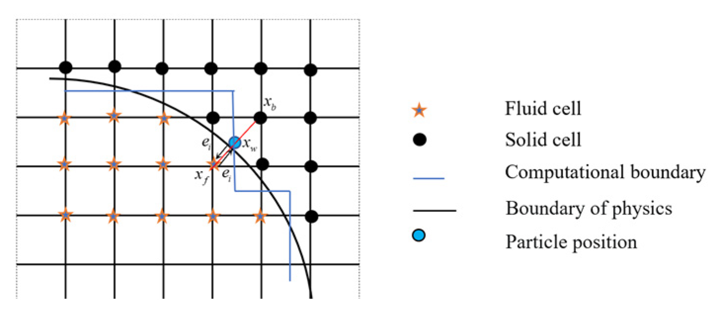
2.4. LBM Boundary Condition

In the flow field, a half-step rebound scheme with second-order accuracy is used for the curve and plane boundary [28], and in the temperature field, we use an anti-rebound boundary condition with second-order accuracy for the heat source surface. Taking the heat source as an example, the unknown velocity distribution function on the right wall surface is as follows:

$$\left\{\begin{array}{c}{f}_{1,n}=f_{3,n}\\ f_{5,n}=f_{7,n}\\ f_{8,n}=f_{6,n}\end{array}\right.$$

(39)

The unknown temperature distribution function at the right boundary of the heat source is as follows:

$$\left\{\begin{array}{c}{g}_{1,n}=\left(w_1+w_3\right)-g_{3,n}\\ g_{5,n}=\left(w_5+w_7\right)-g_{7,n}\\ g_{8,n}=\left(w_8+w_6\right)-g_{6,n}\end{array}\right.$$

(40)

where n represents the lattice node position.

In this paper, a model with a heat source inside a semicircular cavity is proposed, including surface velocity boundary and surface temperature boundary conditions. In LBM, the processing of surface boundaries is more complicated. As shown in Figure 2, the area of the calculation boundary is surrounded by physical nodes. The outside of the calculation domain is the physical boundary. At least one node in the fluid domain intersects with the physical boundary. Therefore, the unknown function is obtained from the intermediate nodes of the solid domain and the fluid domain. Therefore, the position distribution function of the fluid boundary can be expressed as:

$$f_{\overline{i}}(x_w,t)=f(x_w,t) g_{\overline{i}}(x_w,t)=-g(x_w,t)$$

(41)

where $x_w=(x_f+x_b)/2$, $\overline{i}=-i$.

2.5. Average Nusselt Number

The local Nusselt number is defined as:

$$Nu=-\frac{k_{nf}}{k_f}\frac{L}{\Delta T}\frac{\partial T}{\partial n}$$

(42)

where L represents the characteristic length of the thermal wall. $\Delta T=T_h-T_c$ is the temperature difference.

The average Nusselt number represents 1/L of the total Nusselt number of walls.

$$N{u}_{ave}=\frac{1}{L}{\displaystyle {\int }_0^{L}Nu\mathrm{d}n}$$

(43)

According to Equation (43), the $N{u}_{ave}$ on the surface of the heat source is defined herein as its total number on the surface divided by four, which is calculated using the following formula:

$$N{u}_{ave}=\frac{N{u}_{lave}+N{u}_{rave}+N{u}_{uave}+N{u}_{bave}}{4}$$

(44)

where $N{u}_{lave}$, $N{u}_{rave}$, $N{u}_{uave}$ and $N{u}_{bave}$ represent the average Nusselt numbers of the walls of the heat source, respectively.

2.6. Entropy Generation

Under the action of buoyancy drive and Lorentz force, irreversibility occurs in heat transfer ($S_{\theta }$), fluid friction ($S_{\psi }$) and magnetic entropy production rate ($S_m$), which can be expressed as [29]:

$$S_{\theta }=\frac{k_{nf}}{k_f}\left({\left(\frac{\partial \theta }{\partial X}\right)}^2+{\left(\frac{\partial \theta }{\partial Y}\right)}^2\right)$$

(45)

$$S_{\psi }=\chi \frac{{\mu }_{nf}}{{\mu }_f}\left(2\left({\left(\frac{\partial U}{\partial X}\right)}^2+{\left(\frac{\partial V}{\partial Y}\right)}^2\right)+{\left(\frac{\partial U}{\partial Y}+\frac{\partial V}{\partial X}\right)}^2\right)$$

(46)

$$S_m=\chi \frac{{\mu }_{nf}}{{\mu }_f}\frac{{\sigma }_{nf}}{{\sigma }_f}H{a}^2{V}^2$$

(47)

where $\chi =\frac{{\mu }_f{T}_m}{k_f}{\left(\frac{{\alpha }_f}{L\left(\Delta T\right)}\right)}^2$ represents an irreversible factor. The integral form of the total entropy generation is:

$$S_{tot}={\displaystyle {\int }_0^L{\displaystyle {\int }_0^L{S}_{\theta }}}dxdy+{\displaystyle {\int }_0^L{\displaystyle {\int }_0^L{S}_{\psi }}}dxdy+{\displaystyle {\int }_0^L{\displaystyle {\int }_0^L{S}_m}}dxdy=S_{\theta ,{\rm T}}+S_{\psi ,T}+S_{m,T}$$

(48)

The Bejan number represents the proportion of heat transfer irreversibility in the total entropy generation, and is given as:

$$Be=\frac{S_{\theta ,T}}{S_{tot}}$$

(49)

3. Results and Discussion

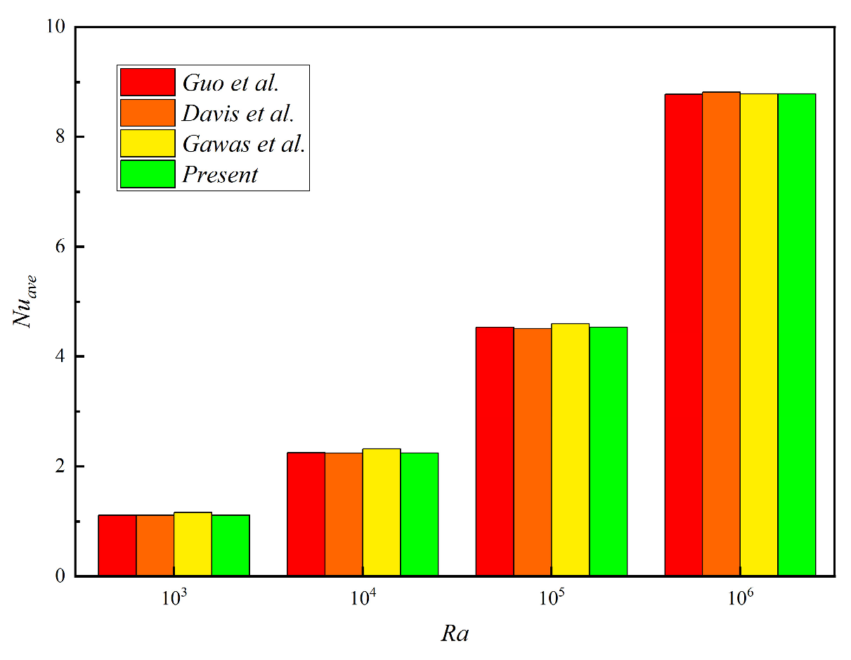
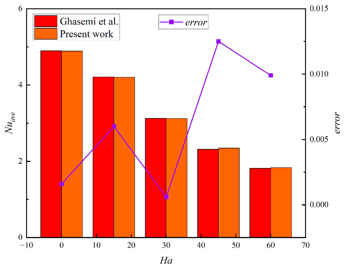
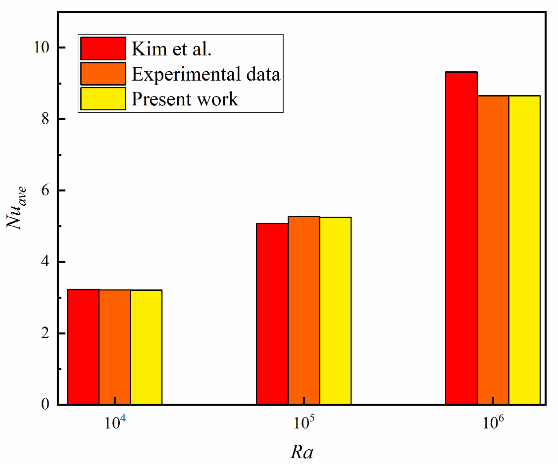
3.1. Model Validation

To verify the correctness of the program, this paper first verified the $N{u}_{ave}$ of the left wall of the heat source and compared it with the previous results. The results are shown in Figure 3, where the maximum error of the average Nusselt number is 3.9%, indicating the correctness of the program. On this basis, this paper further verified the $S_{tot}$ (no magnetic entropy production) and the proportion of irreversible heat transfer in the total entropy generation (Be) in the square cavity, as shown in Figure 4. The results are in good agreement. On this basis, the flow heat transfer of nanofluid containing Al₂O₃ in a square cavity is verified without considering Brownian force. The $N{u}_{ave}$ of the left hot wall surface at $\varphi =0.04$ and $R{\mathrm{a}=10}^5$ under different Hartmann numbers is obtained, as shown in Figure 5, and the maximum deviation is 1.25%. Figure 6 compares the average Nusselt number in this paper with previous work, and the results are in good agreement. Overall, all these consistent results, both qualitative and quantitative, provide convincing evidence of the accuracy of this work and verify the reliability of the program. Therefore, the program can satisfy the study of the natural convection of nanofluids.

3.2. Grid Independence Verification

As shown in Figure 7, this paper selected five grids of different sizes (60 × 60, 80 × 80, 100 × 100, 120 × 120, 140 × 140). In the initial condition of Ha = 30, $\varphi =0.04$, $\gamma =0$, the grid independence is verified by the numerical results of the $N{u}_{ave}$ and the $S_{tot}$. The grid independence verification results are shown in Figure 7. In order to obtain the optimal computational efficiency, 120 × 120 was used for the entire numerical simulation.

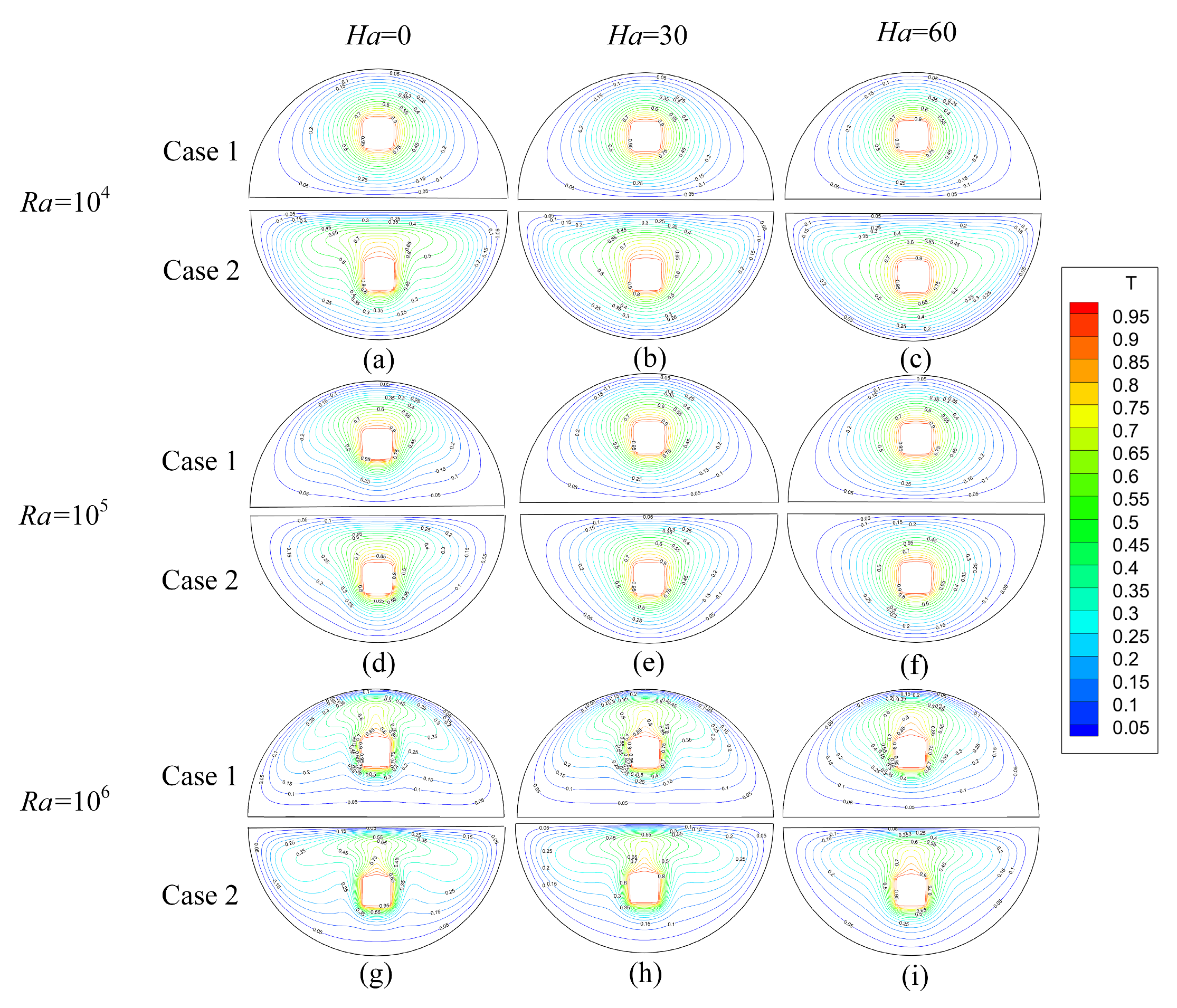
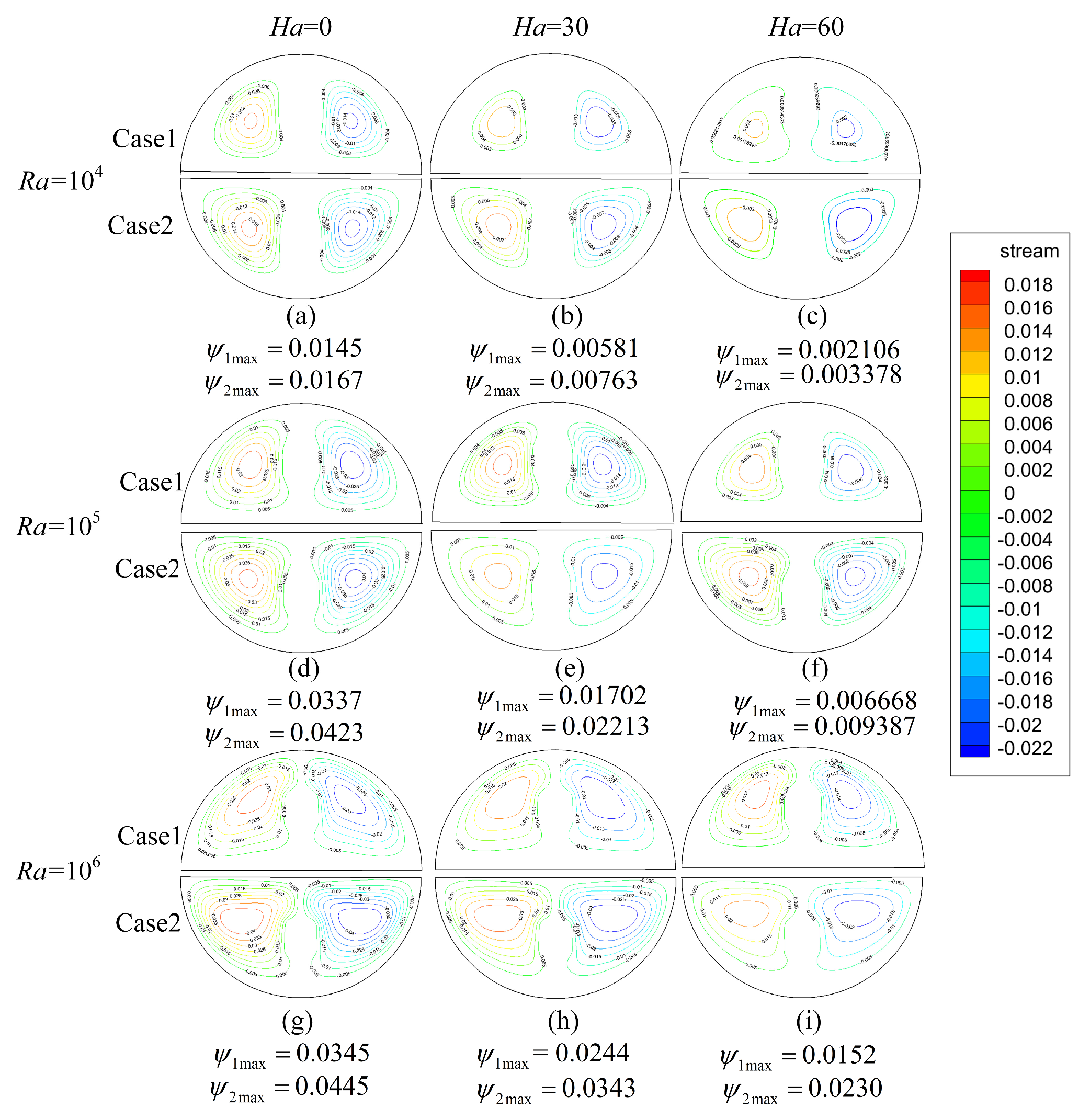
3.3. Influence of Ra and Ha on Flow

When $\gamma =0$ and $\varphi =0.04$, the isotherm distribution of Case 1 and Case 2 is shown in Figure 8. Since the model is left–right symmetric, the isotherm distribution of the model is also left–right symmetric. At this time, the changes in isotherm distribution of Case 1 and Case 2 are similar, so the two cases are put together for discussion. Ra can effectively reflect the influence of thermal buoyancy on the viscosity of nanofluids. When Ra = 10⁴, the isotherms from the heat source to the outside are evenly distributed, and the change in the Ha number has no great influence on the isotherms; that is, the addition of a magnetic field does not have much effect on the way heat is conducted. When Ra = 10⁵, Ha = 0, it is obvious that the isotherms on both sides of the heat source are twisted upward, and the isotherms near the lower wall surface of the heat source and the upper shell form aggregation. With the increase in Ha, the distortion becomes significantly smaller. When Ra = 10⁶, the isotherms are highly concentrated near the cold wall surface, above the heat source and the lower surface of the heat source, which is mainly affected by convection heat transfer. With the increase in Ha, the thermal plume on both sides of the heat source is smaller, and the degree of isotherm distortion above the heat source is reduced. This is due to the magnetic field joining in nanofluids produced perpendicular to the magnetic field of Lorentz force. The number of Ha enhancement can magnify the Lorentz force. When the Ra is small, the main method of heat transfer is thermal conduction and the increase in the magnetic field has little effect on heat conduction and heat transfer. When Ra increases to 10⁶, the buoyancy-driven natural convection begins to increase, and the addition of magnetic field can effectively suppress its intensity.

When $\gamma =0$; $\varphi =0.04$, the streamline distribution diagram and maximum flow function of Case 1 and Case 2 are shown in Figure 9. ${\psi }_{1\max }$ and ${\psi }_{2\max }$ represent the maximum flow functions of Case 1 and Case 2, respectively. It can be seen that since the model is left–right symmetric, the streamline distribution is also left–right symmetric. Since the changes in the streamline distribution of Case 1 and Case 2 are similar, the two cases are put together for discussion. The fluid is guided by the heat source and cooled by the cold surface of the outer wall and two symmetrical counter-rotating flows on both sides of the heat source.

With the increase in Ra, the flow function increases, the vortex center on both sides of the heat source moves upward, and the flow intensity of the vortex center increases. Since the buoyancy-driven flow is stronger than viscous flow at high Ra, the flow function reaches the maximum sum ${\psi }_{1\max }=0.0345$ and ${\psi }_{2\max }=0.0445$. When Ra = 10⁶, the flow function reaches the maximum sum. At the same time, the streamline near the cold wall surface is denser. The increase in Ha can effectively suppress the size of the flow function. At the same Ra, when Ha = 60, the flow function is the smallest. Compared with Case 2, when Ha = 0, the flow function of Case 2 increases by 29% compared to that of Case 1. At a high Rayleigh number, the flow function of Case 2 is inhibited by 8.2% less than that of Case 1; that is, the flow function of Case 2 is inhibited by the Hartman number less than that of Case 1.

3.4. Average Nusselt Number of Heat Source Surface

The $N{u}_{ave}$ represents the functional relationship between Ra, Ha, and $\varphi$. This paper mainly explores the influence of different Ha and Ra on the $N{u}_{ave}$ of the heat source surface and compares the $N{u}_{ave}$ of Case 1 and Case 2.

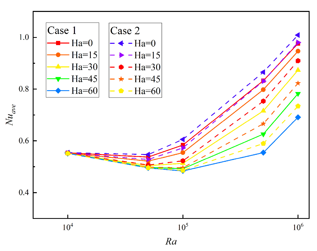
3.4.1. Influence of Ra and Ha on the Average Nusselt Number

Figure 10 shows the influence of Ra and Ha on the $N{u}_{ave}$ at $\varphi =0.04$ and $\gamma =0$. Since the change trends of Case 1 and Case 2 are basically the same, they are analyzed together. Based the figure, we can determine that at a low Ra, the number of Hartmann changes does not effectively change the size of the $N{u}_{ave}$. With the increase in Ra, the $N{u}_{ave}$ first decreases after a sharp rise, ultimately promoting effect, and at the high Ra, the increase in Ha inhibitory effect on the $N{u}_{ave}$ increases. When Ra = 10⁴, Ha has little effect on the $N{u}_{ave}$ of the fluid. When Ra = 5 × 10⁴, the $N{u}_{ave}$ decreases slightly. When Ha ranges from 0 to 60, the decline rate of the $N{u}_{ave}$ gradually increases. The maximum decline rate is at Ha = 60. When Ha = 30, the decline rate of the $N{u}_{ave}$ increases the most. When Ra = 10⁵ and Ha goes from 0 to 30, the $N{u}_{ave}$ increases. When Ha = 0 and Ha = 15, adding a magnetic field cannot obviously improve the heat transfer performance. When $Ha\ge 30$, the magnetic field begins to inhibit the heat transfer performance. When Ra ranges from 10⁵ to 10⁶, the magnetic field can obviously inhibit the improvement of the heat transfer performance. On the whole, the external magnetic field has a negative effect on the heat transfer of nanofluids.

For Case 1 and Case 2, the $N{u}_{ave}$ of Case 2 is significantly larger than that of Case 1 under the same circumstances; that is, the heat transfer effect of Case 2 is better. This is because the flow function of Case 2 is larger than that of Case 1, and the flow of nanofluids is more complex, resulting in greater convection intensity near the heat source in Case 2. In particular, at high Ra, the vortex center range of Case 2 is larger and the overall flow gradient is larger, meaning that it has a better heat transfer effect.

3.4.2. Influence of Magnetic Field Angle and Ha on the Average Nusselt Number

Figure 11 shows the influence of $\gamma$ and Ha at Ra = 10⁵, When $\gamma ={30}^{°}$, the heat transfer performance of nanofluids is the best. When $\gamma =0$ and $\gamma ={60}^{°}$, the average Nusselt number of nanofluids is the lowest. The change in the magnetic field angle can regulate the heat transfer performance of nanofluids to a certain extent, but generally speaking, the control range is small, and the change in the Hartmann number plays a decisive role in the average Nusselt number. Compared with Case 1 and Case 2, under the same conditions, the average Nusselt number of Case 2 increases by 10%. This is mainly because the isotherm dense area exists above the heat source, and the area above Case 2 is larger, which is more conducive to heat transfer.

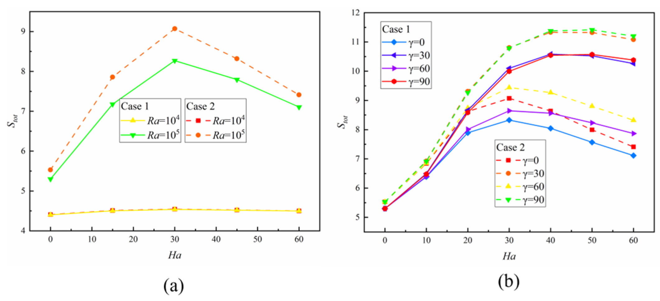
3.5. Total Entropy Generation and Bejan Number

3.5.1. Generation of Entropy

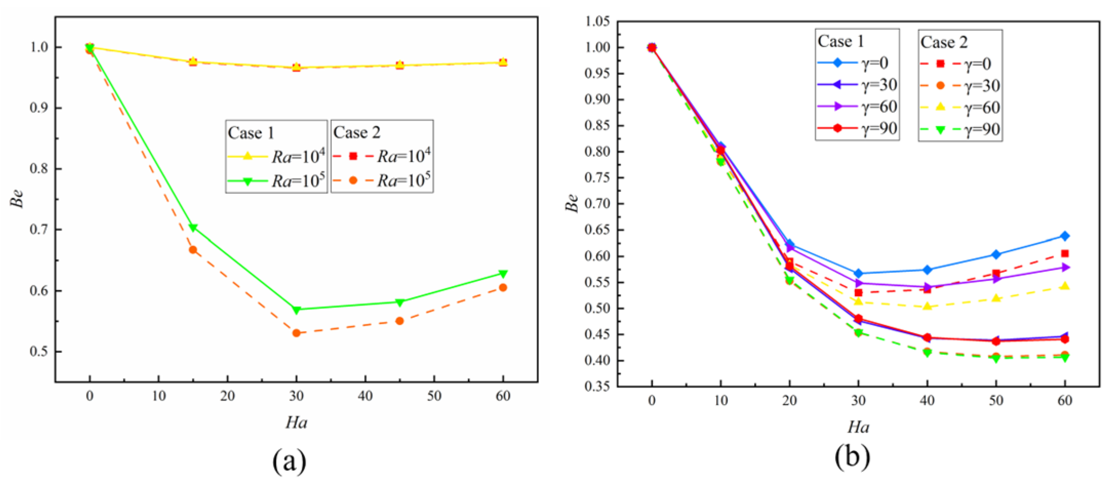
Figure 12a,b shows the relationship between the $S_{tot}$, Ra, Ha, and the magnetic field angle. As shown in Figure 12a, when Ra = 10⁴, the natural convection intensity in the cavity is relatively small and mainly in the state of heat conduction, and the change of Ha has no effect on $S_{tot}$. At this time, $S_{tot}$ of Case 1 and Case 2 is basically the same, and the overall level is at a low level. When Ra = 10⁵, the intensity of natural convection in the cavity and the $S_{tot}$ increases. With the addition of magnetic field, $S_{tot}$ reaches the maximum at Ha = 30. With the continuous increase in Ha, $S_{tot}$ begins to decrease. Compared with Case 1 and Case 2, under the same conditions, $S_{tot}$ of Case 2 is larger than that of Case 1, which is mainly because the natural convection is mainly above the system. The space above the reservoir in Case 2, the intensity of natural convection and $S_{tot}$ are all larger.

As shown in Figure 12b, under the same conditions, when $\gamma {=30}^{°}$ and $\gamma {=90}^{°}$, the $S_{tot}$ is maximum, while $\gamma =0$, $S_{tot}$ is minimum. When Ha increases from 0 to 10, the change of magnetic field angle has little effect on $S_{tot}$. With the further increase in Ha, the influence of magnetic field angle change on $S_{tot}$ further increases. The greater the magnetic field intensity, the greater the influence of magnetic field angle change on $S_{tot}$. When Ha = 40, $\gamma {=30}^{°}$ and $\gamma {=90}^{°}$, $S_{tot}$ reaches its peak. With the increase in Ha, $S_{tot}$ decreases slightly. When Ha = 30, $\gamma =0$ and $\gamma {=60}^{°}$, $S_{tot}$ reaches its peak. With the increase in Ha, $S_{tot}$ decreases significantly compared with other magnetic field angles. Compared with Case 1 and Case 2, the increase range of $S_{tot}$ of Case 2 is larger than that of Case 1, and $S_{tot}$ of Case 2 is larger than that of Case 1, but the change trend of the two models is basically the same under the same conditions.

3.5.2. Bejan Number

The Bejan quantifies the ratio of heat transfer irreversibility to total entropy generation. Figure 13a,b show the relationship between the Bejan number, Ra, Ha, and magnetic field angle. As shown in Figure 13a, when Ra = 10⁴, the system is mainly in heat conduction state, and Be is close to 1, which is a basically irreversible heat transfer in the cavity. When Ra = 10⁵ and Ha = 0, Be does not change with the change in Ra. With the increase in Ha, Be first decreases and then increases, and reaches the minimum value around Ha = 30, at which time $S_{tot}$ reaches the maximum value. Compared with Case 1 and Case 2, when Ra = 10⁴, the Be of Case 1 and Case 2 is the same, and the increase in Ha has little influence on Be. When Ra = 10⁵, the Be of Case 2 is smaller than that of Case 1, the intensity of natural convection in the cavity of Case 2 is larger, and the proportion of irreversible heat transfer is smaller. Under the action of magnetic field, the magnetic field has a greater influence on the Be of large natural convection. When the system is in the state of heat conduction, the magnetic field intensity has little influence on it. As shown in Figure 13b, when Ha increases from 0 to 20, the increase in Ha decreases Be, and the change in the magnetic field angle has little effect on Be. With the increase in Ha, when $\gamma =0$, Be is the largest under the same model, while $\gamma {=30}^{°}$ and $\gamma {=90}^{°}$, Be is the smallest in the same model. The greater the magnetic field intensity, the greater the influence of the magnetic field angle change on Be. Compared with Case 1 and Case 2, under the same condition, the Be of Case 2 is smaller than that of Case 1, the irreversible proportion of heat transfer is smaller, and the $S_{tot}$ is higher under the same condition.

4. Conclusions

The LBM code including KKL was used to study the natural convection of CuO-H₂O nanofluids in a semicircular cavity under the action of a magnetic field. The isothermal heat source was placed in the center of the cavity, while the periphery of the semicircle was kept at a low temperature. The distribution function in LBM was used to solve the governing equations, including velocity, energy and diffusion equations. The effects of Ra, Ha, $\gamma$ and other parameters relating to flow and heat transfer characteristics were considered in detail. Through the analysis of the above results, the following main results were obtained:

• For either Case 1 or Case 2, the increase in Ra makes the isotherm more pinnate and distorted, and the increase in Ha inhibits it. The maximum value of the flow function increases with the increase in Ra and the decrease in Ha. Compared with Case 1 and Case 2, the flow function of Case 2 is larger under the same conditions.
• When Ha ≥ 30, the $N{u}_{ave}$ decreases first and then increases sharply with the Rayleigh number. When Ra = 10⁵ and Ha = 30, the $N{u}_{ave}$ reaches the maximum value when $\gamma ={30}^{°}$. The average Nusselt number of Case 1 is larger than that of Case 2 under the same conditions, and the heat transfer effect of Case 2 is better.
• Under the same Ha, the increase in Ra can promote the increase in $S_{tot}$, when $\gamma =0$ and Ha < 30, $S_{tot}$ is the increasing function of Ha. When Ha = 30, $S_{tot}$ reaches the maximum. With the continuous increase in Ha, $S_{tot}$ is the decreasing function of Ha. Changing the angle of the magnetic field can affect this trend, when $\gamma ={30}^{°}$ and $\gamma ={90}^{°}$, $S_{tot}$ reaches its maximum when Ha = 40. Under the same conditions, $S_{tot}$ in Case 2 is higher than that in Case 1.

References

1. Samipour, S.A.; Khaliulin, V.I.; Batrakov, V.V. Development of the Technology of Manufacturing Aerospace Composite Tubular Elements by Radial Braiding. J. Mach. Manuf. Reliab. 2018, 47, 284–289. [Google Scholar] [CrossRef]
2. Wang, Z.L. Triboelectric Nanogenerators as New Energy Technology for Self-Powered Systems and as Active Mechanical and Chemical Sensors. ACS Nano 2013, 7, 9533–9557. [Google Scholar] [CrossRef]
3. Choi, S.U.S.; Eastman, J. Enhancing Thermal Conductivity of Fluids with Nanoparticles. In Proceedings of the 1995 International Mechanical Engineering Congress and Exhibition, San Francisco, CA, USA, 12–17 November 1995; Volume 66. [Google Scholar]
4. Meghdadi Isfahani, A.H.; Afrand, M. Experiment and Lattice Boltzmann numerical study on nanofluids flow in a micromodel as porous medium. Phys. E Low-Dimens. Syst. Nanostruct. 2017, 94, 15–21. [Google Scholar] [CrossRef]
5. Manna, O.; Singh, S.K.; Paul, G. Enhanced thermal conductivity of nano-SiC dispersed water based nanofluid. Bull Mater. Sci. 2012, 35, 707–712. [Google Scholar] [CrossRef]
6. Chang, H.; Jwo, C.S.; Fan, P.S.; Pai, S.H. Process optimization and material properties for nanofluid manufacturing. Int. J. Adv. Manuf. Technol. 2007, 34, 300–306. [Google Scholar] [CrossRef]
7. Sheikholeslami, M.; Gorji-Bandpy, M.; Seyyedi, S.M.; Ganji, D.D.; Rokni, H.B.; Soleimani, S. Application of LBM in simulation of natural convection in a nanofluid filled square cavity with curve boundaries. Powder Technol. 2013, 247, 87–94. [Google Scholar] [CrossRef]
8. Ghasemi, B.; Aminossadati, S.M.; Raisi, A. Magnetic field effect on natural convection in a nanofluid-filled square enclosure. Int. J. Therm. Sci. 2011, 50, 1748–1756. [Google Scholar] [CrossRef]
9. Nakharintr, L.; Naphon, P. Magnetic field effect on the enhancement of nanofluids heat transfer of a confined jet impingement in mini-channel heat sink. Int. J. Heat Mass Tran. 2017, 110, 753–759. [Google Scholar] [CrossRef]
10. Lee, T.; Lee, J.H.; Jeong, Y.H. Flow boiling critical heat flux characteristics of magnetic nanofluid at atmospheric pressure and low mass flux conditions. Int. J. Heat Mass Tran. 2013, 56, 101–106. [Google Scholar] [CrossRef]
11. Balakin, B.V.; Stava, M.; Kosinska, A. Photothermal convection of a magnetic nanofluid in a direct absorption solar collector. Sol. Energy 2022, 239, 33–39. [Google Scholar] [CrossRef]
12. Khanafer, K.; Vafai, K.; Lightstone, M. Buoyancy-driven heat transfer enhancement in a two-dimensional enclosure utilizing nanofluids. Int. J. Heat Mass Tran. 2003, 46, 3639–3653. [Google Scholar] [CrossRef]
13. Mahmoodi, M. Numerical simulation of free convection of a nanofluid in L-shaped cavities. Int. J. Therm. Sci. 2011, 50, 1731–1740. [Google Scholar] [CrossRef]
14. Sourtiji, E.; Hosseinizadeh, S.F. Heat transfer augmentation of magnetohydrodynamics natural convection in L-shaped cavities utilizing nanofluids. Therm. Sci. 2012, 16, 489–501. [Google Scholar] [CrossRef]
15. He, B.; Lu, S.; Gao, D.; Chen, W.; Li, X. Lattice Boltzmann simulation of double diffusive natural convection of nanofluids in an enclosure with heat conducting partitions and sinusoidal boundary conditions. Int. J. Mech. Sci. 2019, 161, 105003. [Google Scholar] [CrossRef]
16. Saberi, A.H.; Kalteh, M. Two-phase lattice Boltzmann simulation of nanofluid conjugate heat transfer in a microchannel. Thermophys. Aeromech. 2021, 28, 401–419. [Google Scholar] [CrossRef]
17. Alinejad, J.; Esfahani, J.A. Lattice Boltzmann simulation of 3-dimensional natural convection heat transfer of CuO/water nanofluids. Thermophys. Aeromech. 2017, 24, 95–108. [Google Scholar] [CrossRef]
18. Goodarzi, M.; Orazio, A.D.; Keshavarzi, A.; Mousavi, S.; Karimipour, A. Develop the nano scale method of lattice Boltzmann to predict the fluid flow and heat transfer of air in the inclined lid driven cavity with a large heat source inside, Two case studies: Pure natural convection & mixed convection. Phys. A Stat. Mech. Its Appl. 2018, 509, 210–233. [Google Scholar]
19. Ma, Y.; Rashidi, M.M.; Mohebbi, R.; Yang, Z.G. Nanofluid natural convection in a corrugated solar power plant using the hybrid LBM-TVD method. Energy 2020, 199, 117402. [Google Scholar] [CrossRef]
20. Li, J. Computational Analysis of Nanofluid Flow in Microchannels with Applications to Micro-Heat Sinks and Bio-MEMS. Ph.D. Thesis, North Carolina State University, Raleigh, NC, USA, 2008. [Google Scholar]
21. Sheikholeslami, M.; Gorji-Bandpy, M.; Ganji, D.D.; Soleimani, S. Natural convection heat transfer in a cavity with sinusoidal wall filled with CuO–water nanofluid in presence of magnetic field. J. Taiwan Inst. Chem. E 2014, 45, 40–49. [Google Scholar] [CrossRef]
22. Koo, J. Computational Nanofluid Flow and Heat Transfer Analyses Applied to Micro-Systems. Ph.D. Thesis, North Carolina State University, Raleigh, NC, USA, 2005. [Google Scholar]
23. Koo, J.; Kleinstreuer, C. A new thermal conductivity model for nanofluids. J. Nanopart. Res. 2004, 6, 577–588. [Google Scholar] [CrossRef]
24. Pordanjani, A.H.; Jahanbakhshi, A.; Nadooshan, A.A.; Afrand, M. Effect of two isothermal obstacles on the natural convection of nanofluid in the presence of magnetic field inside an enclosure with sinusoidal wall temperature distribution. Int. J. Heat Mass Tran. 2018, 121, 565–578. [Google Scholar] [CrossRef]
25. Koo, J.; Kleinstreuer, C. Laminar nanofluid flow in microheat-sinks. Int. J. Heat Mass Tranf. 2005, 48, 2652–2661. [Google Scholar] [CrossRef]
26. Guo, Z.; Shi, B.; Zheng, C. A coupled lattice BGK model for the Boussinesq equations. Int. J. Numer. Meth. Fluidsuids 2002, 39, 325–342. [Google Scholar] [CrossRef]
27. Qian, Y.H.; D’Humières, D.; Lallemand, P. Lattice BGK Models for Navier-Stokes Equation. Europhys. Lett. 1992, 17, 479. [Google Scholar] [CrossRef]
28. Tao, S.; Wang, L.; Ge, Y.; He, Q. Application of half-way approach to discrete unified gas kinetic scheme for simulating pore-scale porous media flows. Comput. Fluids 2021, 214, 104776. [Google Scholar] [CrossRef]
29. Basak, T.; Kaluri, R.S.; Balakrishnan, A.R. Entropy Generation During Natural Convection in a Porous Cavity: Effect of Thermal Boundary Conditions. Numer. Heat Transf. Part A Appl. 2012, 62, 336–364. [Google Scholar] [CrossRef]
30. De Vahl Davis, G. Natural convection of air in a square cavity: A bench mark numerical solution. Int. J. Numer. Meth. Fluids 1983, 3, 249–264. [Google Scholar] [CrossRef]
31. Gawas, A.S.; Patil, D.V. Rayleigh-Bénard type natural convection heat transfer in two-dimensional geometries. Appl. Therm. Eng. 2019, 153, 543–555. [Google Scholar] [CrossRef]
32. Magherbi, M.; Abbassi, H.; Brahim, A.B. Entropy generation at the onset of natural convection. Int. J. Heat Mass Transf. 2003, 46, 3441–3450. [Google Scholar] [CrossRef]
33. Kashyap, D.; Dass, A.K. Effect of boundary conditions on heat transfer and entropy generation during two-phase mixed convection hybrid Al2O3-Cu/water nanofluid flow in a cavity—ScienceDirect. Int. J. Mech. Sci. 2019, 157, 45–59. [Google Scholar] [CrossRef]
34. Kim, B.S.; Lee, D.S.; Ha, M.Y.; Yoon, H.S. A numerical study of natural convection in a square enclosure with a circular cylinder at different vertical locations. Int. J. Heat Mass Transf. 2008, 51, 1888–1906. [Google Scholar] [CrossRef]
35. Warrington, R.O.; Powe, R.E. The transfer of heat by natural convection between bodies and their enclosures. Int. J. Heat Mass Tran. 1985, 28, 319–330. [Google Scholar] [CrossRef]
Figure 1. Model and boundary conditions.
Energies 16 04055 g001
Figure 2. Schematic diagram of half-step rebound method.
Energies 16 04055 g002
Figure 3. Comparison of the average Nusselt number of the left hot wall of natural convection in a square cavity with Guo et al. [26], Davis et al. [30] and Gawas et al. [31] ( P r = 0.71 ).
Energies 16 04055 g003
Figure 4. Comparison of the total entropy generation (no magnetic entropy production) and Bejan number of natural convection in the cavity under different Rayleigh numbers with Magherbi et al. [32] and Kashyap et al. [33] ( P r = 0.71 ).
Energies 16 04055 g004
Figure 5. Comparison of average Nusselt number of the left hot wall filled with Al2O3-H2O nanofluid under different Hartmann numbers with Ghasemi et al. [8].
Energies 16 04055 g005
Figure 6. Comparison of the average Nusselt number between present data with Kim et al. [34] and Warrington et al. [35] ( P r = 0.71 ).
Energies 16 04055 g006
Figure 7. Comparison of the S t o t and N u a v e under different grid sizes and Rayleigh numbers ( H a = 30 ,   ϕ = 0.04 ,   γ = 0 ).
Energies 16 04055 g007
Figure 8. Isotherm distribution of Case 1 and Case 2 under different Ra ( 10 4 ) and Ha ( 0 H a 60 ).
Energies 16 04055 g008
Figure 9. Streamlines distribution and maximum flow function of Case 1 and Case 2 under different Ra ( 10 4 R a 10 5 ) and Ha ( 0 H a 60 ).
Energies 16 04055 g009
Figure 10. Average Nusselt numbers of Case 1 and Case 2 under different Ra and Ha.
Energies 16 04055 g010
Figure 11. Effect of magnetic field angle and Ha on the N u a v e .
Energies 16 04055 g011
Figure 12. (a) Effects of Ra and Ha on Stot at γ = 0 (b) Effects of Ha and γ on Stot at Ra = 105.
Energies 16 04055 g012
Figure 13. (a) Effects of Ra and Ha on the Be at γ = 0 (b) Effects of Ha and γ on the Be at Ra = 105.
Energies 16 04055 g013