Abstract
This paper proposes a model predictive controller (MPC) design based on the optimal tip-speed ratio method for maximum power point tracking (MPPT) of a direct-driven permanent magnet synchronous generator (D-PMSG)-based wind energy conversion system (WECS). To eliminate system nonlinearity and time-varying characteristics, a control variable was added at the wind turbine and the system model was feedback-linearized to create a linear time-invariant system, reducing the computational burden of the MPC and improving system performance. MATLAB/Simulink simulations were performed and the results show that the linearized system has high fidelity. Compared to traditional MPC that use an operating point to linearize the system, it has better adaptability to turbulent wind speeds, improving the stability and rapidity of the system.
1. Introduction
Wind turbines are an effective renewable energy generation devices, with minimal emissions and reduced environmental pollution compared to traditional fossil fuel power generation methods [1,2,3,4,5]. Among them, (D-PMSG)-based wind turbines have received extensive attention due to their superiority. Its rotor is composed of permanent magnets and uses direct drive to generate power, without the need for mechanical transmission devices, such as gears, reducing the failure rate of the wind turbine. Additionally, it has the advantages of small size, low noise, and high efficiency [6,7,8,9]. However, the harsh working environment still presents challenges for their stable operation.
In order to improve the stability and energy conversion efficiency of wind turbines, a method combining grey prediction and PI controller was proposed in [10]. The predicted value obtained by grey prediction was used as the input of the PI controller, together with the deviation from the given value, to adjust the power output of the wind turbine. The simulation results showed that the designed system had the characteristics of fast response and small overshoot. In [11], a combined optimization control method based on ant colony algorithm and PI controller was proposed to obtain better PI controller coefficients. The parameters were optimized using the optimization algorithm. The simulation results showed that this method can effectively improve the power generation efficiency of wind turbines. Ref. [12] proposed a control strategy combining grey wolf optimization and PI controller to better track the maximum power point of wind turbines by calculating the parameters of the PI controller through the optimization algorithm. The above literature used other algorithms combined with PI controller to achieve good control effects. However, for multi-parameter systems, such as wind turbines, achieving constraints on some variables and solving the dead zone problem with PI control is difficult. To suppress disturbances in nonlinear systems, ref. [13] combined sliding mode control and fuzzy control technology to design a controller that can achieve the required performance. The simulation results showed that this method enhances the robustness of wind turbines. The accurate measurement of an effective wind speed is a key task that has a significant impact on the output power, safety, and control performance of wind turbines. Ref. [14] trained an artificial neural network using the least squares method and backpropagation gradient descent algorithm to accurately estimate the effective wind speed without using any mechanical wind speed sensors. The MATLAB simulation results demonstrated the accuracy and reliability of the estimator, and the effectiveness of the method was demonstrated by the simulation testing of a 5 MW offshore wind turbine system. Due to the inherent inertia, wind turbine rotors cannot immediately respond to changes in wind speed. Therefore, ref. [15] proposed using the time-series adaptive linear prediction (ALP) technique to improve the lag of wind turbines. The simulation results showed that this method improved the wind turbine power generation efficiency by nearly 5%. The methods mentioned in the above articles can improve the performance of wind turbines, but the design is relatively difficult and the implementation in engineering is challenging, which can add considerable uncertainty in complex environments.
With the development of artificial intelligence technology, this technology has been applied to wind turbines. A reinforcement learning-based adaptive optimal fuzzy controller was proposed in [16]. The critic used an adaptive neuro-fuzzy inference system (ANFIS) network instead of a traditional neural network for the construction process, in order to reduce computation. Additionally, the proposed controller is output feedback instead of state feedback, which does not require system models and parameters, thus exhibiting robustness to system uncertainties and external disturbances. The feasibility of the method was verified through simulations. In [17], a training model based on a recursive neural network was proposed to reduce wind speed measurement errors. A method combining rotor speed control and pitch angle control was also proposed to better achieve the maximum power point tracking (MPPT) problem. The effectiveness of the control system was demonstrated through simulation experiments on a 5 kW wind turbine model. Different intelligent control strategies for wind turbine blade pitch angle control were introduced in [18]. Neural networks and reinforcement learning were used to control the pitch angle of wind turbines, aiming at the nonlinearity of wind turbine systems and the interference of external environments. Some application examples were presented in the article, proving the feasibility of the methods. A specific learning algorithm was designed in [19] to adjust neuron weights online, while most previous articles trained networks offline. This method can effectively reduce errors caused by wind speed changes to the system. The simulation experiments on a 1.5 MW wind turbine in the article showed that the wind turbine power increased by 7.87%.
In recent years, the method of combining MPC with wind turbines has been proposed. The MPC control algorithm is an advanced control method that can accurately predict the behavior of the control system, minimize losses, and meet various constraints, effectively dealing with various problems faced by wind power generation. The MPC control method can consider multiple factors, such as wind speed, rotor speed, power generation, and power factor. through model optimization prediction, making the wind turbine system more stable, efficient, and reliable. To reduce the impact of wind speed fluctuations on the stable operation of the wind turbine, ref. [20] treated wind speed random fluctuations as bounded disturbances and used the Robust Model Predictive Control (RMPC) strategy to limit the state of the wind turbine system within a certain range. The simulation results showed that it can effectively reduce the impact of wind speed changes on the stable operation of the turbine and improve the quality of power generation. In order to enable the semi-submersible floating wind turbine to operate stably under various complex working conditions, ref. [21] designed and constructed a Gain-Scheduling Multi-Model Predictive Controller (GM-MPC). The simulation experiments were conducted under various wind-wave joint loads, and the results showed that the wind turbine reduces the mechanical load of the unit while ensuring power stability. Both of these studies achieved good control results, but they used the equilibrium point linearization method when linearizing the system, which is only accurate near the equilibrium point. When the external environment changes, there will be distortion problems in the system. Ref. [22] established a small-signal model of the wind turbine system, and the simulation results showed that the system is stable when experiencing disturbances of step-down and step-up in wind speed. The dynamic response of the system is consistent with the small-signal analysis results. In view of the dual time-scale characteristics of the wind power generation system, ref. [23] decomposed the wind turbine system into fast and slow subsystems based on singular perturbation theory, and applied the continuous MPC algorithm to control the two subsystems separately. A Kalman filter was designed for noise. According to the simulation results, this method effectively improved the power generation efficiency of the wind turbine. However, there is no accurate method for decomposing the fast and slow subsystems. A continuous MPC algorithm will introduce derivative and integral operations, which add computational pressure to the system. Moreover, the parameter adjustment of a continuous MPC is very difficult, which is not conducive to engineering implementation.
Based on the above analysis, the nonlinearity and time-varying nature of wind turbines are the challenges of implementing MPC control. Currently, the mainstream method is to use the steady-state linearization method. However, it is difficult to select the equilibrium point, and the model only has high fidelity around the equilibrium point. When the system deviates from the equilibrium point, the previously selected model becomes distorted. When facing turbulent wind speeds, the equilibrium point continuously changes. To ensure the model’s authenticity, the calculated model needs to be continuously updated, which adds a considerable computational burden to the MPC control system and introduces system lag.
To solve this problem, this paper adds a control variable to the system, and uses feedback linearization to eliminate the nonlinear part and time-varying parameters of the system. The obtained linear system calculates the virtual control rate through MPC, and then obtains the actual control rate through the feedback equation, which acts on the actual nonlinear system. The structural schematic diagram is shown in Figure 1.
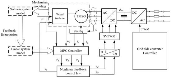
Figure 1.
Model predictive control system based on feedback linearization.
By using MATLAB/Simulink simulation, the results show that the (MPC) system based on feedback linearization is superior to the MPC controller using the linearization around an operating point, with improved speed and stability. The main work of this paper is as follows:
- (1)
- The mathematical modeling of (D-PMSG)-based wind turbines is carried out based on the mechanism modeling method.
- (2)
- A novel controller is introduced to perform feedback linearization processing on the system, eliminating the nonlinear part and time-varying parameters. The obtained system is discretized. Through simulation, the fidelity of the system is proved by comparing it with the original system.
- (3)
- Design an MPC controller, the system is simulate using MATLAB/Simulink and the results are observed.
2. Modeling of (D-PMSG)-Based wind Turbines
2.1. Wind Turbine Model
The power extracted from the wind can be represented as:
where is the air density in , is the area swept by the fan blades in [], is the wind speed, in , and is the optimal coefficient for wind energy utilization, whose approximate value, obtained from [24], is:
where, as a function, represents the pitch angle of the blades and represents the tip-speed ratio, where R is the blade rotation radius measured in [m] and is the angular velocity of the blade rotation measured in [rad/s]. The expression for is:
The mechanical torque, denoted as and measured in [N m], can be obtained by the ratio of mechanical power and angular velocity [25]:
2.2. Drive Train Model
The drive train of a wind turbine can be treated as a model with a concentrated mass at a single point, which can yield a highly accurate analytical model. The rotational dynamics of this system can be expressed as a second-order differential equation [26]:
where is the combined inertia of the turbine and generator in [kg ], is the damping coefficient of the turbine in [kg /s], is the electromagnetic torque of the generator in [N m], is the rotor speed of the Permanent Magnet Synchronous Generator (PMSG), and , where is the gearbox transmission ratio. In PMSG, there is no gearbox, hence = 1. The dynamic equation for rotor speed is expressed as:
2.3. Permanent Magnet Synchronous Generator Model
Electric motors with windings having a sinusoidal distribution are typically mathematically modeled using the dq-axis framework, consisting of two equivalent circuits, each on one axis. The dq-axis coordinate system is used to analyze the transient and steady-state performance of permanent magnet synchronous generators.
The instantaneous voltage and current of the synchronous generator’s phases a, b, and c constitute the three-phase variables of the abc coordinate system. They can be transformed into two-phase variables in a reference system defined by mutually perpendicular d and q axes. The dq-axis fame has an arbitrary position relative to the abc-axis fame, rotates at a speed of , and is determined by the angle between the a-axis and d-axis. The balanced three-phase voltages , , and in the abc coordinate system can be equivalently transformed into the rotating dq-axis fame through inverse Park and Clarke transformations [27].
where and represent the d-axis and q-axis voltage, respectively, and represents the zero-sequence voltage. The zero-sequence variable is related to the symmetrical component:
In the balanced condition, , therefore , which means that the zero-sequence component can be ignored in the dq-axis coordinate system.
The voltage equation of a permanent magnet synchronous generator (PMSG) can be expressed using the aforementioned transformation, with the angular speed in the motor’s measured reference frame serving as the electrical angular frequency [24], represented as:
where and are the stator currents in [A], and are the stator voltages in [V], and is the stator resistance in []. is the electrical angular frequency of the generator in [rad/s], and it is equal to
where is the number of magnetic poles in a permanent magnet synchronous generator (PMSG). and are the stator magnetic flux linkages in [Wb]. The stator magnetic flux linkage can be represented as
where and are the stator inductances on the d-axis and q-axis in [H]. is the magnetic flux linkage of the permanent magnet. By inputting the stator magnetic flux linkage into the voltage equation, we obtained:
The equation is converted into a differential equation form [28] and substituted in (10):
For non-salient pole PMSG, = [29], the electromagnetic torque is expressed as:
3. MPC Controller Design Based on Feedback Linearization
In this section, the feedback linearization technique is used to transform the model of the fan system into a linear model, thereby reducing the computational burden of MPC, improving system performance, and making it more feasible for engineering implementation.
3.1. Design of MPC
MPC (Model Predictive Control) is an algorithm based on predicting future states based on the current system state, typically used for controlling discrete-time linear time-invariant systems. Compared to the traditional PI closed-loop control, MPC has the advantages of a fast dynamic response and good parameter optimization [30]. The key concept of MPC is to use a system model to predict the future states of the system. Consider the following system:
the prediction horizon is set to in the process of prediction:
Equation (16) can be written in a more concise form:
where:
In the control process, it is desired that the system can accurately track the set value and the control variable is as smooth as possible [31]. Therefore, the quadratic cost function is written as:
where:
Because the objective is to minimize the cost function , if more emphasis is placed on the system’s tracking ability, the elements in the matrix can be set to be larger, which can make the system reach the set value faster but unavoidably causes larger overshoots. However, if it is desired to avoid rapid changes in the system control variable or to save energy, the elements in the matrix can be set to be larger, but this increases the time for the system to reach the set value. Additionally, if it is desired to handle a specific state or control variable, the corresponding weight values can be changed. Equation (17) can be substituted into (19), thus obtaining the results for:
The quadratic function is calculated to obtain the control sequence . Only the first term is applied to the system [32]. The resulting new state is used in Equation (16) to achieve rolling optimization.
3.2. System Feedback Linearization Design
According to Equations (6), (13), and (14), (D-PMSG)-based wind turbines are described as:
The system state and input variables are defined as:
From Expression (22), we obtained the following:
- The system exhibits obvious nonlinearity. The mainstream approach to deal with nonlinear systems is to linearize the system using the equilibrium points. However, the selection of equilibrium points is difficult, and the equilibrium points also change with the variation of wind speed, which affects the accuracy of the system.
- The system is a time-varying system. In order to achieve a maximum power point tracking, the wind turbine needs to keep the generator speed at , where . Therefore, as the wind speed changes, also changes accordingly. This means that the matrices and in Equation (18) also change in real time. In other words, when the wind speed changes, the controller needs to calculate the system reference values based on the current wind speed and compute the new and values. This introduces a delay to the system.
This article considers using feedback linearization to turn the system into a linear system and eliminate time-varying parameters. Since the system’s control variables and cannot directly affect , an additional controller is added. Here, represents the friction coefficient, is a negative coefficient, and is a small positive number. According to [33], the stability margin of the system and the friction coefficient have a linear relationship within a certain range. Therefore, by controlling the friction within a certain range, the system’s stability can be improved. The resulting system with an additional controller is expressed as:
Equation (24) is expressed in the form of a nonlinear system [34]:
The linear feedback design for (25) can be obtained by rewriting the control variable as:
The new system representation in the state-space form is:
The system thus becomes a linear system, and the time-varying parameters are eliminated.
3.3. Feedback Linearization Feasibility Analysis
3.3.1. Lyapunov Stability Analysis
To analyze the stability of the system (26), consider a Lyapunov quadratic candidate function:
where is a diagonal matrix and is the system state variable.
The matrix is positive definite and symmetric, where , , and are positive. It satisfies the condition for a Lyapunov candidate function. The system matrix is represented by , considering that the derivative of with respect to time is negative definite, that is:
Lemma 1.
When , there exists a negative definite symmetric matrix that satisfies the Lyapunov condition:
Proof of Lemma 1.
matrix is:
The order of the matrix’s leading principal minors can be obtained based on the conditions of Lemma 1.
As all , , , , , , , are positive, is negative definite, is positive definite, and is negative definite. is a negative definite and diagonal matrix. The and matrices satisfy the Lyapunov equation. Therefore, the system is stable. □
3.3.2. System Equivalence Analysis
The system obtained after feedback linearization was discretized to obtain a linear time-invariant (LTI) discrete system. We used MATLAB/Simulink to build the original system and the LTI system, inputting the same signal to both systems and observing the response curve. The obtained response curves are shown in Figure 2 and Figure 3.
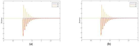
Figure 2.
Response when the input is a step signal. (a) Original system; (b) LTI system.
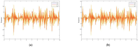
Figure 3.
Response when the input is a high-frequency oscillation signal. (a) Original system; (b) LTI system.
The results indicate that the system has similar dynamic characteristics to the original system for step and high-frequency signals. By eliminating non-linear terms and time-varying parameters and , designing an MPC controller at this point without the need for real-time updates of and can improve the system’s response speed and accuracy.
4. Simulation Results and Analysis
To verify the feasibility of the theory, the simulation testing of a 300 kW direct-drive permanent magnet synchronous wind turbine generator was carried out using MATLAB/Simulink. The parameters of the (D-PMSG)-based wind turbines are shown in Table 1.

Table 1.
The wind turbine and generator parameters.
Wind speed sequences were simulated within the range of 8 m/s to 15 m/s using MATLAB, as shown in Figure 4.
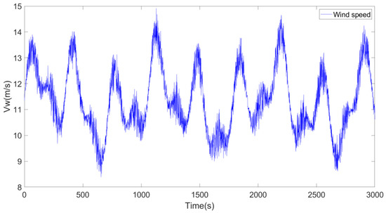
Figure 4.
Simulation of wind speed sequences.
A comparison was made between a wind turbine control system based on Feedback Linearization Control (FLC) and Model Predictive Control (MPC), and a MPC wind turbine control system based on Linearization about an Equilibrium Point (LEP), using the method described in [35] for LEP. The selection of parameters is described in Appendix A. The comparison was carried out for maximum power point tracking under the wind speed shown in Figure 4, and the simulation results are shown in Figure 5, Figure 6 and Figure 7.
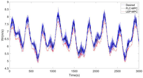
Figure 5.
Comparison of the rotational speed.
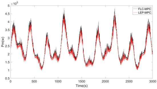
Figure 6.
Comparison of power.
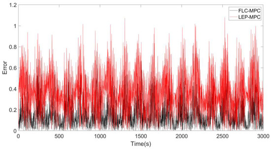
Figure 7.
Comparison of the error in rotational speed to the expected speed.
Figure 5 and Figure 6 demonstrate that the combination of feedback linearization and MPC can achieve faster and more accurate maximum power point tracking, resulting in a higher power generation. As mentioned in [36], the efficiency of the wind energy conversion system was used as a performance metric, which is defined as the ratio of actual output power to theoretical power. This can be expressed as shown in (34).
where and are the theoretical power and actual power of the WECS, respectively, and is the overall system efficiency. According to calculations, the results presented in Table 2 are obtained.
Table 2.
Numerical analysis of the power generation efficiency.
Figure 7 shows that using feedback linearization can reduce the error. Based on the comprehensive analysis of performance indicators, such as root-mean-square error (RMSE), mean absolute error (MAE), relative error (RE), and maximum deviation (MAX DEV), the results obtained are shown in Table 3.
Table 3.
Numerical analysis of error.
According to the results, the combination of feedback linearization and MPC can make the wind turbine track the maximum power point more quickly and accurately, effectively improving the system’s dynamic performance. This increases the average wind energy capture efficiency and power generation efficiency of the wind turbine.
5. Conclusions and Future Works
In recent years, the MPC algorithm has gradually been used in wind power generation systems due to its easy-to-adjust parameters and good control effect. However, MPC places a significant demand on computation, especially in controlling nonlinear and time-varying systems. This article proposed the use of feedback linearization to linearize wind power systems, solving the difficulties of system nonlinearity and time variation. Compared with the equilibrium point linearization method, it greatly reduces the amount of computation required and is more conducive to engineering implementation. The simulation results show that the feedback-linearization-based MPC wind energy conversion system has a good control performance in simulated wind speed sequences. Compared with MPC control systems processed by equilibrium point linearization, it has a faster response speed, can better track the optimal speed, and effectively improves the average wind energy capture efficiency and power generation efficiency.
As for our future work, the analysis of the impact of friction on the wind turbine system will be conducted to determine the values of and b using a more scientific method. Regarding the idea of controlling friction, there is currently no suitable actuator available. Furthermore, for wind turbines, multiple types of turbines will be considered in future studies.
Author Contributions
Conceptualization, P.J., T.Z., J.G., P.W. and L.F.; Methodology, P.J., T.Z., J.G. and P.W.; Software, L.F.; Writing—original draft, P.J., T.Z., J.G., P.W. and L.F.; Writing—review & editing, P.J., T.Z., J.G., P.W. and L.F. All authors have read and agreed to the published version of the manuscript.
Funding
The APC was funded by Natural Science Foundation of Hebei Province, grant number A2020201021; Central Government Guides Local Science and Technology Development Fund Project, grant number 226Z2103G; and Natural Science Foundation of Hebei Province, grant number F2020201014.
Data Availability Statement
Not applicable.
Conflicts of Interest
The authors declare no conflict of interest.
Appendix A
The selection of the important parameters for the method presented in reference [35] is shown below.
Selection of the Lie derivative:
The representation of the nonlinear system is expressed by:
where:
The Lie derivatives are:
where:
Thus, we obtain:
In order to transform the system into a normal form, a coordinate transform, fulfilling the diffeomorphism condition, must be found:
Solving for:
Therefore:
where:
The control input:
where:
Thus, we obtain:
Selection of and :
In order to ensure zero error in the steady-state regime, an integrator was added. Defining the extended state vector , the linear system is:
The control input was obtained as:
Thus, the closed-loop system is described by:
, and were calculated using a pole-placement technique. According to (A15), the transfer function of the system can be obtained as:
Thus, a dominant pair of poles was imposed, defined by the cut-off frequency and the damping factor . The corresponding characteristic equation should be:
The dominant poles can be obtained as:
To reduce the impact of the other pole on the system, the real part should be at least five times larger than the dominant pole. Therefore, the pole selection is:
Based on the poles, we can determine:
References
- Hamatwi, E.; Davidson, I.E.; Gitau, M.N.; Adam, G.P. Modeling and Control of Voltage Source Converters for Grid Integration of a Wind Turbine System. In Proceedings of the IEEE PES Power Africa Conference, Livingstone, Zambia, 28 June–2 July 2016. [Google Scholar]
- Hua, G.; Dewei, X. Stability Analysis and Improvements for Variable-Speed Multipole Permanent Magnet Synchronous Generator-Based Wind Energy Conversion System. IEEE Trans. Sustain. Energy 2011, 2, 459–467. [Google Scholar]
- Ran, Z.; Lianxue, G. Research on the design and optimization of 1.5 MW semi-direct drive permanent magnet synchronous wind turbine. In Proceedings of the International Conference on New Energy and Power Engineering, Sanya, China, 19–21 November 2021. [Google Scholar]
- Lu, P.; Ye, L.; Tang, Y.; Zhang, C.; Zhong, W.; Sun, B.; Zhai, B.; Qu, Y.; Liu, X. Multi-time Scale Active Power Optimal Dispatch in Wind Power Cluster Based on Model Predictive Control. Proc. CSEE 2019, 39, 6572–6582. [Google Scholar]
- Saberi, S.; Rezaie, B. Robust adaptive direct speed control of PMSG-based airborne wind energy system using FCS-MPC method. ISA Trans. 2022, 131, 43–60. [Google Scholar] [CrossRef] [PubMed]
- Neelam, M.; Jaffery, M.H.; Jawad, M. A new predictive control strategy for improving operating performance of a permanent magnet synchronous generator-based wind energy and superconducting magnetic energy storage hybrid system integrated with grid. J. Energy Storage 2022, 55, 105515. [Google Scholar]
- Krishna, V.B.M.; Sandeep, V. Experimental investigation on performance comparison of self excited induction generator and permanent magnet synchronous generator for small scale renewable energy applications. Renew. Energy 2022, 195, 431–441. [Google Scholar] [CrossRef]
- Nerg, J.; Ruuskanen, V. Lumped-parameter-based thermal analysis of a doubly radial forced-air-cooled direct-driven permanent magnet wind generator. Math. Comput. Simul. 2013, 90, 218–229. [Google Scholar] [CrossRef]
- Liu, S.; Li, S.; He, L. Direct-driven Permanent Magnet Synchronous Wind-power Generating System with Two Three-level Converters Based on SVPWM Control. Procedia Eng. 2012, 29, 1191–1195. [Google Scholar] [CrossRef]
- Wang, M.; He, S.; Li, X.; Li, Z. Grey Prediction PI Control of Direct Drive Permanent Magnet Synchronous Wind Turbine. Water Resour. Power 2021, 39, 189–192. [Google Scholar]
- Mokhtari, Y.; Rekioua, D. High performance of maximum power point tracking using ant colony algorithm in wind turbine. Renew. Energy 2018, 126, 1055–1063. [Google Scholar] [CrossRef]
- Yang, B.; Zhang, X.; Yu, T.; Shu, H.; Fang, Z. Grouped grey wolf optimizer for maximum power point tracking of doubly-fed induction generator based wind turbine. Energy Convers. Manag. 2017, 133, 427–433. [Google Scholar] [CrossRef]
- Wang, R.; Jiang, H.; Zhao, Y.; Wang, C.; Wei, M. Fuzzy sliding mode control design for the stabilization of wind power generation system with permanent magnet synchronous generator. Energy Rep. 2022, 8, 1530–1537. [Google Scholar] [CrossRef]
- Asghar, A.B.; Liu, X. Adaptive neuro-fuzzy algorithm to estimate effective wind speed and optimal rotor speed for variable-speed wind turbine. Neurocomputing 2018, 272, 495–504. [Google Scholar] [CrossRef]
- Narayana, M.; Sunderland, K.M.; Putrus, G.; Conlon, M.F. Adaptive linear prediction for optimal control of wind turbines. Renew. Energy 2017, 113, 895–906. [Google Scholar] [CrossRef]
- Vu, N.T.T.; Nguyen, H.D.; Nguyen, A.T. Reinforcement Learning-Based Adaptive Optimal Fuzzy MPPT Control for Variable Speed Wind Turbine. IEEE Access 2022, 10, 95771–95780. [Google Scholar] [CrossRef]
- Anto, A.Y.; Young, H.J.; Seong, R.L. Reference Model Adaptive Control Scheme on PMVG-Based WECS for MPPT under a Real Wind Speed. Energies 2022, 15, 3091–4007. [Google Scholar]
- Sierra-García, J.E.; Santos, M. Neural networks and reinforcement learning in wind turbine control. Rev. Iberoam. Autom. E Inf. Ind. 2021, 18, 327–335. [Google Scholar] [CrossRef]
- Muñoz-Palomeque, E.; Sierra-García, J.E.; Santos, M. Wind turbine maximum power point tracking control based on unsupervised neural networks. J. Comput. Des. Eng. 2022, 10, 108–121. [Google Scholar] [CrossRef]
- Zhang, J.; Liu, L.; Liu, Y.; Zhu, Y.; Yan, J. Research on Robust Model Predictive Control Strategy of Wind Turbines to Reduce Wind Power Fluctuation. Electr. Power Syst. Res. 2022, 213, 108945. [Google Scholar] [CrossRef]
- Song, Z.; Feng, H.; Yu, Z.; Hu, Y.; Liu, J. Coordinated Control of Semi-submersible Floating Turbine with Model Predictive Control Strategy. Proc. CSEE 2022, 42, 4330–4339. [Google Scholar]
- Huang, H.; Mao, C.; Lu, J.; Wang, D. Small-signal modelling and analysis of wind turbine with direct drive permanent magnet synchronous generator connected to power grid. IET Renew. Power Gener. 2012, 6, 48–58. [Google Scholar] [CrossRef]
- Zhang, Y. Analysis and Synthesis of Several Classes of Singularly Perturbed Systems. Ph.D. Thesis, Nanjing University of Science & Technology, Nanjing, China, November 2015. [Google Scholar]
- Nguyen, P.T.H.; Stüdli, S.; Braslavsky, J.H.; Middleton, R.H. Lyapunov stability of grid-connected wind turbines with permanent magnet synchronous generator. Eur. J. Control 2022, 65, 100615. [Google Scholar] [CrossRef]
- Ma, W. Modeling and Simulation for Direct-Drive Permanent Magnet Wind Power System. Master’s Thesis, Lanzhou University of Technology, Lanzhou, China, April 2010. [Google Scholar]
- Li, H.; Zhu, C.; Fan, Z.; Tan, J.; Song, C. Research on maximum power point tracking strategy of wind turbine based on second order sliding model-PID control. Acta Energ. Sol. Sin. 2022, 43, 306–314. [Google Scholar]
- Grenier, D.; Louis, J.P. Modeling for control of non-sinewave permanent-magnet synchronous drives by extending Park’s transformation. Math. Comput. Simul. 1995, 38, 445–452. [Google Scholar] [CrossRef]
- Mahmud, M.A.; Roy, T.K.; Littras, K.; Islam, S.N.; Amanullah, M.T. Nonlinear Partial Feedback Linearizing Controller Design for PMSG-Based Wind Farms to Enhance LVRT Capabilities. In Proceedings of the IEEE International Conference on Power Electronics, Drives and Energy Systems, Chennai, India, 18–21 December 2018. [Google Scholar]
- Zhang, Z.; Zhao, Y.; Qiao, W.; Qu, L. A Discrete-Time Direct-Torque Control for Direct-Drive PMSG-Based Wind Energy Conversion Systems. IEEE Trans. Ind. Appl. 2015, 51, 3504–3514. [Google Scholar] [CrossRef]
- Dong, L.; Chen, H.; Pu, T.; Chen, N.; Wang, S. Multi-time Scale Dynamic Optimal Dispatch in Active Distribution Network Based on Model Predictive Control. Proc. CSEE 2016, 36, 4609–4617. [Google Scholar]
- Guo, H.; Yang, J.; Zhang, X.; Cui, j. Model predictive control strategy based on feedback linearization for brushless doubly fed machine. Acta Energ. Sol. Sin. 2020, 41, 342–348. [Google Scholar]
- Éverton, L.; Renato, M.M. Disturbance-Observer-Based Model Predictive Control of Underwater Vehicle Manipulator Systems. IFAC-Pap. 2021, 54, 348–355. [Google Scholar]
- Mahmud, M.A.; Hossain, M.J.; Pota, H.R.; Zhang, C. Investigation of Critical Factors Affecting Dynamic Stability of Wind Generation Systems with Permanent Magnet Synchronous Generators. IFAC Proc. Vol. 2014, 47, 7665–7670. [Google Scholar] [CrossRef]
- Lin, H.; Wang, Y.; Ji, H. Model Predictive Control of PMSM Based on Feedback Linearization. Meas. Control Technol. 2011, 30, 53–57. [Google Scholar]
- Munteanu, I.; Bratcu, A.I.; Cutululis, N.-A.; Ceangă, E. Optimal Control of Wind Energy Systems, 1st ed.; Springer: London, UK, 2009; pp. 150–157. [Google Scholar]
- Hassanien, R.; Abdel-Raheem, Y.; Hossam, H.H.M.; Essam, E.M.M. An efcient variable-step P&O maximum power point tracking technique for grid-connected wind energy conversion system. SN Appl. Sci. 2019, 1, 1658–1672. [Google Scholar]


Disclaimer/Publisher’s Note: The statements, opinions and data contained in all publications are solely those of the individual author(s) and contributor(s) and not of MDPI and/or the editor(s). MDPI and/or the editor(s) disclaim responsibility for any injury to people or property resulting from any ideas, methods, instructions or products referred to in the content. |
© 2023 by the authors. Licensee MDPI, Basel, Switzerland. This article is an open access article distributed under the terms and conditions of the Creative Commons Attribution (CC BY) license (https://creativecommons.org/licenses/by/4.0/).