1. Introduction
Frequency response analysis (FRA) is a well-known monitoring and diagnostic method used in the industry to detect faults in power transformers [
1,
2,
3]. This technique is based on interpreting power transformers as an electric circuit comprising inductive, capacitive, and resistive parameters. When a fault occurs inside the transformer, these parameters are differently influenced. For example, short-circuited turns can affect self and mutual inductances, while winding movements can principally affect series capacitances [
4]. A comparison between reference measurement (before fault or healthy measurement) and actual measurement (faulty measurement) presents frequency response deviations because of circuit parameter change. These deviations can therefore allow fault identification.
Nonetheless, FRA interpretation is not straightforward. This is because the parameters in frequency response depend on many variables in the transformer design characteristics, such as power and voltage ratios, insulation type, winding types, and connections. In this regard, many researchers have been focusing on developing objective interpretation schematics to identify fault type, extent, and location [
5,
6,
7,
8]. The main categories of interpretation methods are numerical indices, simulation models, and automatic classification algorithms [
9].
The use of numerical indices helps quantify the difference between reference and actual measurement. This technique has been applied using numerical index limits to differentiate healthy and faulty transformers [
10,
11,
12] and as an input to automatic classification algorithms [
6,
13].
High-frequency simulation models are used to reproduce the power transformer response. These models allow the generation of FRA traces at different fault conditions without damage to the physical transformer. The simulations to obtain transformers’ frequency response can use the finite element method (FEM) [
14,
15] and the RLC equivalent circuit method [
16,
17,
18], individually or combined [
4], to recreate the traces.
The equivalent RLC circuits use lumped elements such as resistances, self and mutual inductances and capacitances estimated from analytical calculations, or FEM simulations [
16,
19,
20,
21,
22]. Lumped-circuit elements are widely used in various transformers/inductors modelling applications [
23,
24]. Alternatively, simulation models can also be used to detect change in lumped circuit parameters in faulty conditions [
4]. FEM simulations have advantages over analytical formulas, such as the calculation of parameters from complex and anisotropic structures. The more detailed the design data introduced to the FEM simulations, the more accurate the estimations the model will present. However, detailed models will also demand higher computational performances.
The current literature on simulation models explores methods to replicate FRA traces and study frequency response simulated traces once faults are introduced [
14]. New information can be acquired by correlating circuit elements changes, or the geometry changes, in previous and after fault simulations [
18,
25,
26]. Moreover, most recent research has also compared the capabilities of simulation models in attaining numerical indices values, to the ones calculated from measured traces [
14].
The FRA method has expanded its use worldwide as a main diagnostic method and, even though it has been standardized by different international groups [
27,
28], the data available to develop and improve the classification of faults is still scarce [
9].
This research has developed a new method for simulating frequency response in transformers using the finite element method (FEM) and lumped circuit elements to contribute to this matter. The approach is based on calculating, estimating, and optimizing lumped circuit parameters. Furthermore, the study also correlates the lumped circuit parameters changes with the different faults that are introduced in the simulated model. This correlation allows for the future study of faults classification and location, that can be developed by using the simulation method, and for further improvement in objective FRA interpretation research.
Based on this analysis, the main contributions of this study are:
A new approach using FEM simulation and lumped circuit analysis to obtain frequency response in transformers;
An optimization method to improve the assessment of the capacitances derived from the high-frequency transformer model;
The characterization of faults based on the lumped element parameter variation;
An approach tailored for generating infinite and unique data with potential impact on FRA interpretation.
2. FEM Modelling and Parameter Estimation
The methodology employed for the frequency response simulation is based on a laboratory winding-model specially designed for FRA measurements. The simulation is first performed using Comsol Multiphysics
® version 5.5 software and, later, the capacitance parameters are optimized using MATLAB
® functions and Comsol Multiphysics
®. The flowchart presented in
Figure 1 helps to illustrate and better understand the methodology used.
2.1. Laboratory Winding-Model
The transformer model consists of two coils, an outer winding (winding 1) and an inner winding (winding 2). A picture of, and the electrical connections schematics for, the winding-model are presented in
Figure 2. The model is specially designed for FRA measurements. Thus, no power or voltage ratings are attributed to it. The insulation present in the winding is uniform, solid, and non-graded. Winding 1 has 300 mm of internal diameter and is composed of 448 turns distributed in 16 sections of 28 turns each. The sections in winding 1 are disposed in the top of the other with pressboard paper spacers of 6.14 mm between them. The total height of winding 1 is 515 mm. Winding 2 has 251 mm of internal diameter with 228 turns distributed in three layers of 76 turns each. The total height of winding 2 is 530 mm.
The 16 sections of winding 1 are designed to be interchanged and, therefore, allow the introduction of faults in the winding-model. For example, short-circuits can be introduced by connecting the terminals of any section. Axial displacements can be created by displacing the entire winding 1, while radial deformation can be performed by exchanging the winding sections for deformed ones, preserving the model’s integrity [
6].
2.2. Frequency Response Simulation
The numerical simulation is performed in three steps. Firstly, a geometric model is developed based on the laboratory winding-model dimensions. Then, the windings are defined using the magnetic fields and electrostatic physics available in Comsol Multiphysics®. These physics are used to associate the geometric sections to the corresponding number of turns and excitations of the coils, as well as the equations that define the study. Finally, an equivalent electric circuit is utilized to obtain the winding’s frequency response.
Figure 3 presents the 2D axis-symmetric and a cut view of the 3D form. A 2D axis-symmetric geometry can be used to represent the model, and this simplification saves computational effort, while the final frequency response is not affected due to the axisymmetric structure of the transformer in its healthy condition.
The inductances of the model are calculated from the magnetic field physics using FEM simulations. To introduce the frequency dependence of self and mutual inductances a turn-based geometry is employed, as shown in
Figure 3c. Furthermore, the FEM simulation considers the skin and proximity effects. Any increase in the frequency is reflected in the current density in the conductors due to these effects. As shown in
Figure 4, at 60 Hz, the current density is primarily uniform in the conductor. As the frequency increases, the current density limits itself to the edges of the conductors.
The series capacitances are calculated from the electrostatic physics using Maxwell’s equation in (1):
where
is the total electric energy,
is the electric flux density,
is the electric field intensity,
is the capacitance and
is the voltage applied. A small voltage (1 V) is then applied between the upper and lower layers of each section of the windings in order to calculate the capacitances values, as illustrated in
Figure 5.
Similar to the series capacitances calculation, the inter-winding capacitances are calculated from the electrostatic physics using Equation (1) by applying the voltage between the two windings of the model.
The admittance (
) to be introduced in the equivalent electric circuit is then determined by Equation (3) [
16]:
where
is the relative permittivity of the insulation material.
Finally, the magnetic field and electrostatic physics in Comsol Multiphysics
® use Ohm’s law to calculate the lumped element parameters. These parameters are then introduced in the electrical circuit physics to calculate the frequency response, similar to the measurement setup presented in
Figure 6. For the measurement setup, as shown in
Figure 6b, the FRA measurement instrument terminals (red and black connectors) are connected to both ends of winding 1 while leaving winding 2 opened. The grounding leads of both connectors are connected together to the ground to provide a reference for the measurement.
A voltage signal of 10 V over a sweep of frequencies is applied to the electric circuit through the input terminal (
), and the measured voltage is obtained at the output terminal (
). The open circuit measurement was preferred due to its extensive applicability in FRA interpretation methods. While winding 1 is under measurement, winding 2 is kept open, according to the FRA measurements standards [
28].
2.3. Optimization of Circuit Parameters
An optimization method is used to obtain the best fit between the measured and simulated curves. This optimization is important to improve capacitance values for the lumped element circuit. One of the major advantages of this optimization method is the possibility to simulate FRA traces even without design details of the transformers’ insulation materials and its physical characteristics. The design information is often not fully disclosed from manufacturers, which can become a problem in the transformers’ model design.
At first, the capacitance values are estimated from the simple geometric parameters of the transformer windings, as described in
Section 2.2, and later the values can be adjusted to obtain an improved reproduction of the FRA traces of the winding-model. The optimization is then performed by using MATLAB
® function fminsearch. Fminsearch uses the Nelder–Mead simplex algorithm, described in [
29].
Initially, the three capacitances estimated by the FEM simulation are the initial values introduced in the algorithm (, , and ). The function makes a simplex evaluation around these initial estimated values (), adding 5% to each of the initial estimations) at a time. Following this, the algorithm modifies the simplex repeatedly until the method finds the minimum of the desired function.
For this research, the mean square error is used as the function to be minimized, and the relative permittivity values (, and , corresponding to the series capacitance of winding 1, 2 and the parallel capacitance between them) are the variables ().
The optimization adjusts the relative permittivity values at each interaction. The new capacitance values are then re-introduced in the lumped element circuit and the simulated frequency response is recalculated. The mean square error between measured and new simulated curves is obtained until the error is minimal. The optimization ends once , which means the error function has reached a local minimum.
2.4. Evaluation of Simulation Model
Different faults are introduced to evaluate the simulation model created. Four extents of axial displacement (AD) fault, and two short-circuit (SC) faults, are generated in the simulated model. These two fault types are sufficiently different and diversified to exploit the capabilities of the simulated model. As discussed in the literature and the simulation process, axial displacements influence series and inter-winding capacitances, while short-circuit faults influence winding inductances and resistances [
3,
30]. The variation of the lumped circuit elements after fault introduction is later explored in this research.
The axial displacement fault is created by inserting spacers at the bottom of winding sections (below section 16) to displace the whole winding axially, resulting in a loss of magnetic coupling between the windings.
The short-circuit fault is created by short-circuiting sections of the winding. Two short-circuit fault scenarios are considered (SC1 and SC2) which correspond to short-circuiting sections 1 and 2 of the winding-models illustrated in
Figure 1b, respectively.
Table 1 illustrates the introduced AD and SC faults along the winding. Both faults have been introduced along the outer winding of the case study model transformer. Further descriptions of the faults’ introduction on this physical transformer winding-model can be found in the literature [
6].
The further objective of the FRA method is to identify, classify and localize faults inside the windings of a power transformer. The computational simulations improve the data available for analysis and so help in understanding the phenomena behind the traces. To contribute to this matter, the simulations developed in this research are evaluated to identify the variations of circuit element parameters inside the windings. The objective of this analysis is to characterize the fault type using the values of the lumped circuit elements compared to those of the reference case (no-fault simulation).
Thus, to attain this objective, the lumped circuit elements (inductances and capacitances) are evaluated over the complete frequency range of simulation, and a root square mean is calculated to characterize each equivalent element of the circuit for each one of the 16 sections. Since the faults are introduced in winding 1, and all the FRA traces considered are accessed with winding 2 in open circuit condition, only the elements of the winding 1 are observed in this analysis.
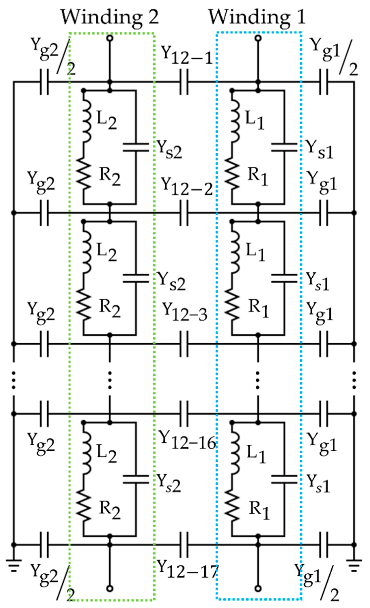
3. Simulated Frequency Response of the Winding-Model
The 16-sections lumped element circuit shown in
Figure 7 is used to obtain the frequency response trace for the winding-model from the simulation. Due to the winding-model specifications, a 16-sections circuit is used comprising series inductances and resistances from winding 1 (
and
, respectively) and winding 2 (
and
, respectively), along with series admittances (
and
), inter-winding admittances (
) and ground admittances (
and
).
The admittances are then optimized to obtain a better fit between simulated and measured FRA traces. Thus, the simulation method can also be applied when sufficient information about the insulation of the transformer windings is unavailable. At first, the relative permittivity is estimated to be one. The calculated admittances considering this relative permittivity are then introduced into the electric circuit to calculate the model’s frequency response. The ground admittances are small and negligible for this winding-model since there is no ground structure near the windings. The measurements are taken inside a Faraday cage with larger dimensions than the winding height. Thus, to complete the electrical circuit presented in
Figure 7, the ground admittances are considered as
.
The initial frequency response obtained from the electrical circuit corresponding to the transformer’s healthy condition is shown in
Figure 8. As can be observed, the curves have similar trends, and the main resonances and anti-resonances are present in the simulated frequency response. However, the absolute error between the curves has considerable values, especially at the resonance points. The mean square error for the curves presented in
Figure 8 is
. This indicates that, although the simulation and circuit models well represent the frequency response of the laboratory winding-model, the initial admittances can still be adjusted to reach a better fit. Thus, there is a need to optimize the simulation parameters.
The optimization is performed and, after about one hundred interactions, the fminsearch obtains the new mean square error of 2.9. The optimization minimizes the mean square error between measured and simulated curves that is calculated from 1 kHz to 1 MHz. The final optimized frequency response is presented in
Figure 9. It can be easily observed from
Figure 9 that the main resonances are still present; they were shifted to better reproduce the measured FRA trace and the error between curves is considerably lowered.
The comparison between measured and simulated curves presented in
Figure 9, reveals that, at higher frequencies close to 1 MHz, measured and simulated curves still present slight amplitude deviations. It is well known from the literature that, around 1 MHz, the frequency response is greatly influenced by the measurement setup [
9,
28], which can be very difficult to reproduce using simulation methods. Nonetheless, for this transformer winding-model, studies have already been presented showing that this region is less affected by faults such as axial displacements and radial deformations [
6].
Only the capacitance values were optimized in this study, although the optimization method could also be applied to inductive and resistive circuit elements. After the first frequency response obtained from the simulation method, it was understandable that the inductance and resistance parameters were well represented by the FEM calculations, since the lower frequency regions (up to 10 kHz) that are influenced by these parameters [
28] presented a good match between measured and simulated traces in
Figure 8.
4. Winding-Model Fault Analysis
To evaluate the model’s performance in reproducing FRA traces of the faulty transformer, four levels of axial displacement and two levels of short-circuit faults were introduced on the transformer’s winding. The fault specifications were discussed and presented earlier in
Table 1. After the fault’s introduction on the winding-model, the frequency response obtained from simulations and compared with the measurements are presented in
Figure 10. In
Figure 10a,b, it is possible to observe that the simulation has very slight deviations for the first axial displacement level. However, once the displacement increases, it is possible to better recognize the deviations due to the fault, especially at frequencies ranging from 400 kHz to 600 kHz; the deviation pattern is clearer at this frequency window, as seen in
Figure 10b. Although the measured and simulated patterns are not perfectly matched, especially at a zoomed-in view, the deviations presented at each axial displacement level follow the same shift pattern and so it is possible to distinguish the extent of each fault.
Figure 10c,d illustrate the two levels of short-circuit fault introduced on the transformer’s windings. At the zoomed portion presented in
Figure 10d, it is possible to clearly see the variations caused by the introduction of the short-circuit fault.
Following this, the circuit elements are obtained from the numerical simulation. The series inductances for each section of winding 1 are presented as
in
Figure 7.
Figure 11 illustrates all the circuit elements extracted from the simulations for each fault. The elements presented in
Figure 11 are normalized using the healthy simulation trace as reference. Therefore, each element is divided by its corresponding reference simulation. The series inductances of winding 1 (
Figure 11a) are represented as
in
Figure 7.
The series capacitances of winding 1 (
Figure 11b) are extracted from the admittances
and the inter-winding capacitances are extracted from
. The inter-winding capacitances represented in
Figure 7 are, in fact, a combination of two adjacent sections, as follows:
where
is the inter-winding admittance set after section (
) and before section (
), and
is the inter-winding admittance of section (
) set between winding 1 and winding 2. Meanwhile, the inter-winding capacitances presented in
Figure 11 are, in fact, the inter-winding capacitances associated with each section and, so, are extracted from
.
It is possible to observe that, in the case of axial displacement faults, the inductances of the sections vary according to a linear line with respect to the reference, as shown in
Figure 11a. The slope of the mentioned line is correlated with the severity of the axial displacement. This can be directly correlated to the variation of the inductive coupling between windings once the displacement of winding 1 increases. Thus, the sections on the top of the winding (as presented in
Figure 2) have more significant variations (up to 20%). Regarding short-circuit faults, the inductance of sections has greater variation, especially where the fault is located. The short-circuit introduced a change largely equivalent to the inductance of the winding and, so, changed the inductances of all the sections.
In general, series capacitances vary slightly (less than 5% variation) except in the case of short-circuits, where capacitors in series tend to have very high values at fault locations, which is normal for a short-circuit.
Finally, the inter-winding capacitances for short-circuit faults were not affected. Meanwhile, for the axial displacement fault, the inter-winding capacitances were greatly affected, especially at winding extremities (sections 1 and 16). The maximum variation observed of 30% occurred for AD 4, which represents 6.7% (34.4 mm/515 mm) of the axial displacement of winding 1.
A further comparison of the two sets of traces presented at
Figure 10, and their circuit elements analyzed in
Figure 11, clearly indicates that the short-circuit faults are more easily detected by the FRA response as they affect the leakage inductance of the transformer immensely, while the effect of the displacement on the distributed parameters of the winding is slight and only a large level of the axial displacement can make a noticeable difference in the trace. Therefore, the detection of this fault type needs more consideration and interpretation in practice. Furthermore, observing the frequency responses presented
Figure 10, it is noticeable that the first resonance point (around 50 kHz) remains almost unaltered for any fault applied. The reason for this behaviour can be justified by the fact that the first resonance point is related to the magnetizing inductance of the transformer and faults such as axial displacements do not considerably affect this parameter.
5. Conclusions
This paper reports a new method for frequency response simulation with an optimization of capacitance parameters to fit measurement and simulation traces. The method’s main objective is to access transformers’ frequency response to develop and improve FRA interpretation techniques. The proposed simulation method uses FEM to obtain inductive and resistive transformer parameters and uses the Nelder–Mead simplex algorithm to optimize values for the relative permittivity parameters. Thereafter, the parameters are integrated into lumped electrical circuit elements, and the circuit’s transfer function is calculated to obtain the model’s frequency response. The results indicate good agreements between the measured and simulated traces.
Due to its destructive nature, faulty measurements cannot be performed in real transformers. Using a laboratory model combined with simulation methods appears to be an interesting approach to contribute to the development of objective FRA interpretation. The proposed approach opens the door for obtaining fault measurements on a single unit and generating a database of frequency responses. The method can further characterize the variation of lumped circuit parameters with respect to the fault introduced in the transformer’s winding. This approach can further be explored to identify and locate faults using FRA.
The method presented in this study demonstrates the use of simulations to obtain frequency response traces for power transformers. The use of the FEM simulation method has many advantages, including the introduction of faulty traces in a healthy transformer without submitting the asset to physical damage. The further use of the proposed method can help in anticipating the behavior of FRA traces in the occurrence of a fault in the windings. This may help in developing and improving objective methods to detect fault occurrences. Additionally, the understanding of parameter changes in the lumped element equivalent circuit obtained from simulated traces can contribute to the determination of fault location and intensity from simulated and measured traces.
Furthermore, the method can also be used to study other types of power transformer windings. The 2D axis-symmetric geometric model allows the reliable representation of any cylindrical type of winding (such as helical and disc types). However, to improve the representation of transformer cores and the influence of multiple phases on simulated FRA traces, a 3D model should be considered. Despite this, the 3D geometric model considerably increases computational effort and simulation time. Thus, a more simplified model should be applied whenever the design allows.


 ,
, 


