Abstract
The future power grid will have more distributed energy sources, and the widespread access of distributed energy sources has the potential to improve the energy efficiency, resilience, and sustainability of the system. However, distributed energy, mainly wind power generation and photovoltaic power generation, has the characteristics of intermittency and strong randomness, which will bring challenges to the safe operation of the power grid. Accurate prediction of solar power generation with high spatial and temporal resolution is very important for the normal operation of the power grid. In order to improve the accuracy of distributed photovoltaic power generation prediction, this paper proposes a new distributed photovoltaic power generation prediction model: ROLL-GNN, which is defined as a prediction model based on rolling prediction of the graph neural network. The ROLL-GNN uses the perspective of graph signal processing to model distributed generation production timeseries data as signals on graphs. In the model, the similarity of data is used to capture their spatio-temporal dependencies to achieve improved prediction accuracy.
1. Introduction
With the rapid growth of energy demand, environmental and energy security issues have attracted more and more attention. As an innovative energy generation mode, distributed generation has rapidly developed in recent years. Therefore, accurate prediction of distributed generation is of great significance to realize the balance of power supply and demand [1,2,3,4]. Improving the ultra-short-term power prediction accuracy of distributed photovoltaic (PV) power is the premise to ensure the safe and stable operation of the distribution network and the reliable consumption of high proportions of distributed PV power. Photovoltaic power generation depends on local weather conditions and cloud dynamics. The generation, movement, and ablation of clouds in the sky are the main reasons for the instability of photovoltaic power output. The accurate analysis of the presence and movement of clouds is the key to the ultra-short-term power prediction of photovoltaic power [5,6,7].
A literature review on existing PV power prediction was implemented. A series of methods considering both satellite images and meteorological data perform well in long-term prediction [8,9,10,11]. By using surface cameras and satellite images, the cloud dynamic information of the sky can be obtained by processing and analyzing the timeseries images of the sky through digital image processing technology [12,13,14]. For example, a mirror gradient repair method is used to restore the cloud distribution in the real sky [15]. Distortion correction was carried out on the ground-based cloud map [16] to improve the radiation prediction accuracy. Through digital image processing technology, the timeseries image of the sky is processed and analyzed [17], and the cloud extraction algorithm [18] is used to predict the solar occlusion, followed by predicting the irradiance and PV power. A PV ultra-short-term power prediction model [18], combining numerical weather prediction and the ground-based cloud map, can be established to predict and correct the power attenuation caused by cloud occlusion. A mathematical model of irradiance conversion and the photovoltaic module model were verified by experiments [19,20,21,22]. Open operation, quadratic polynomial fitting, gray-level segmentation analysis, centroid angle function, and cluster analysis are used to establish the cloud feature model [23,24,25], and then to carry out ultra-short-term photovoltaic power prediction. Although scholars have carried out a lot of work in cloud analysis and feature modeling and ultra-short-term prediction of photovoltaic power based on cloud analysis and modeling in recent years, there are still problems of difficult modeling [26], and the cost of deploying and maintaining ground cameras in power grids with a large number of photovoltaic power stations is high [27,28,29,30,31].
Using historical operation data to obtain the state information of atmospheric clouds is another mainstream direction, which can capture cloud cover and cloud movement by considering the spatial–temporal relationship between PV sites [32,33,34]. To this end, the convolutional neural network (CNN) is used to extract spatio-temporal correlations [35,36,37]. The method is to stack PV signals into images and reorder their positions in the images according to their positions. In addition, the authors of [38,39] also introduced an attention mechanism to capture spatial correlation. Graph signal processing is an emerging field that allows the processing of signals defined by irregular domains by using graphs to capture the interdependencies between PV power generation units in distributed generation areas [40,41,42,43,44].
In recent years, the graph neural network (GNN) has been widely studied in the prediction word of many fields [45,46,47], such as traffic prediction, weather forecast, social media prediction, etc. Due to its powerful expression ability and complex data processing ability, the graph neural network can make each node of the graph structure carry out efficient information transmission. The graph neural network has also been extensively studied in the field of photovoltaic power generation prediction. For example, the timeseries of photovoltaic power production at multiple sites is modeled as the signal on the graph [48,49,50]. The graph neural network and the long- and short-term memory recurrent neural network were combined into a spatio-temporal GNN model to analyze the temporal and spatial characteristics of the historical data of photovoltaic power stations [26,50,51]. However, when the prediction model is faced with the fluctuation of power generation, the fluctuation of the predicted value always lags behind that of the actual value.
Although the above studies use the historical information of each PV power generation point of distributed generation, they do not consider the information transmission direction of each PV power generation node in the distributed generation and cannot make full use of the advanced information of auxiliary PV power generation points. As a result, when the forecasting model faces the fluctuation of power generation, the fluctuation of the predicted value always lags behind the fluctuation of the real value.
Facing the challenge that the fluctuation of the predicted value of photovoltaic power generation always lags behind the fluctuation of the true value, we propose a rolling prediction model based on the graph neural network. The original contribution can be summarized as the following three points:
- Facing the feature that ‘the fluctuation of the predicted value always lags behind the fluctuation of the real value in the time axis’, this paper attempts to use generation power from neighboring PV panels surrounding the target panel to indicate the lagging information in the prediction model.
- The indicated lagging information is generated by a proposed lead–lag relationship analysis on the correlation model. The output of this model is set to the adjacency matrix in the graph neural network.
- As the sun position and the cloud condition change in real time, this paper creates a rolling graph neural network, which uses the latest real-time lead–lag relationship result. The numerical study shows that the proposed rolling graph neural network performs better than typical traditional prediction models.
2. Model Architecture and Mathematical Modeling
The ROLL-GNN model periodically updates the input data of the model to the latest historical power data over time, which leads to different models in different periods, and the structure is the same in each period, including a similarity analysis model and a graph convolutional model.
The similarity analysis model uses the historical data between different power points to calculate the similarity, which can obtain the lead–lag relationship between the data of each power generation point.
The graph convolution model extracts information from the input historical power data according to the adjacency matrix.
2.1. ROLL-GNN
In a suitable period, the lead–lag relationship between the PV power generation units in the distributed generation area is fixed, and this lead–lag relationship can be represented by the adjacency matrix in the graph neural network model. However, over a long period of time, the movement of the cloud layer does not have a single regularity, because of the complex change of the wind direction, and the movement of the cloud layer shows a change of pattern. Therefore, it is represented by multiple different adjacency matrices. Different patterns correspond to different prediction model parameters. We used online rolling training to obtain the adjacency matrix corresponding to this pattern by using the most recent data through similarity analysis. This adjacency matrix determines the direction of information transmission in the graph neural network model, which can reflect the cloud movement law in the current mode. The overall method is shown in Figure 1.
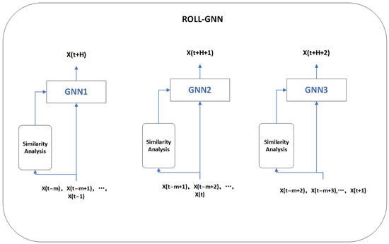
Figure 1.
Schematic diagram of the rolling model.
Figure 1 shows the pattern of rolling predictions. The input for the first period is: X (t − m), X (t − m + 1), …, X (t − 1), and the output is: X (t + H). As the period changes, the input for the second period is: X (t − m + 1), X (t − m + 2), …, X (t), and the output is: X (t + H + 1). In the same way, the input in the third period is: X (t − m + 2), X (t − m + 3), …, X (t + 1), and the output is: X (t + H + 2). The input and output changed with the change of the period, and the similarity analysis model also obtained different adjacency matrices with the change of the input and output, which determined that the graph neural network in different periods was different. It should be noted that the model in the current period was trained on the basis of the model parameters in the previous period. For different forecasting periods, the adjacency matrix was obtained by similarity analysis based on recent historical data, which led to different forecasting models in different periods, which determined the use of rolling forecasting. The specific mathematical formulation is as follows:
where, S represents the similarity calculation, p(t) represents the true value at time t, P(t) represents the predicted value at time t, N represents the observation length of the correlation analysis, M represents the observation length of the graph convolution, and H represents the length of the discrete time steps after the prediction.
The above shows the rule of rolling prediction on the whole timeseries. The schematic diagram for the network structure is shown in Figure 2.
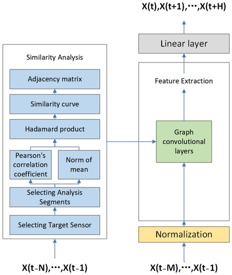
Figure 2.
Schematic diagram of the network structure.
Figure 2 shows the principle of ROLL-GNN in one cycle. The model is divided into two structures: similarity analysis and shape feature extraction.
The similarity analysis model includes several links. First, the target point was selected from all the distributed photovoltaic power generation points. Then, the analysis fragments were extracted from the historical data of the target photovoltaic power generation points. The Pearson correlation coefficient and mean-norm calculation of the target fragments were respectively calculated with the historical data of other photovoltaic power generation points. Then, the similarity curve was obtained by multiplying the calculated results of Pearson correlation coefficient and the mean-norm. Finally, the adjacency matrix was obtained by analyzing the similarity curve.
The feature extraction model is composed of graph convolutional layers, and it extracts features from the input historical data according to the direction of node information flow provided by the adjacency matrix.
2.2. Similarity Analysis
Short-term photovoltaic power generation is mainly affected by cloud movement, which is regular. This movement law can be reflected by the lead–lag relationship between the collected data of different sensors in a plane, as shown in Figure 3, so that the state of the target sensor can be predicted in advance through the auxiliary sensor and the prediction accuracy can be improved. In view of the large amount of information of auxiliary sensors, in order to effectively extract the information with advance prompts, the similarity analysis of the data between the PV power generation units in the distributed generation area can be used to obtain the lead and lag order in the short term. In this paper, the Pearson correlation coefficient and the mean one norm were combined to analyze the data of each PV point, similarly [42].
where, C represents the degree of correlation, n represents the length of the analysis fragment, xi represents the numerical value in the analysis fragment, yi represents the numerical value of the target fragment, X represents the mean value of the whole analysis fragment, and Y represents the mean value of the whole target fragment.
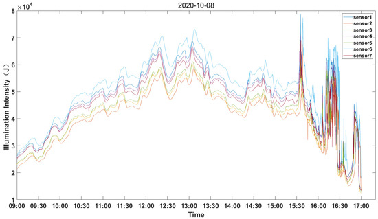
Figure 3.
Schematic of the sensor data.
The process of data processing for correlation analysis is shown in the similarity analysis structure in Figure 2. Firstly, we selected the target PV power generation point at the distributed generation point. In order to improve the accuracy of similarity, we intercepted the fluctuation segment of a fixed length (100 s) in the historical data of the target PV power generation point and calculated the similarity coefficient with the segment of the same length in the fixed period (3600 s) of the data of other PV power generation points. The segment with the largest similarity coefficient was selected as the segment corresponding to the target analysis segment. According to the position of the corresponding segment in the timeline, all PV power generation points can be sorted by leading and lagging in a cycle. Through the above similarity analysis, we can obtain the time ordering of all PV power generation points in the distributed generation area, and it is stipulated that the two PV power generation nodes closest to each other in time can transmit information; that is, the two nodes are connected. If the two nodes are connected, they will have a value of 1 at the corresponding position of the adjacency matrix of the graph neural network; conversely, they will have a value of 0 at the corresponding position of the adjacency matrix of the graph neural network.
2.3. Graph Convolution
A graph is a data structure that represents relationships between entities, where entities are represented by nodes and relationships are represented by edges. Here, a node is denoted by V and an edge by E. The topology of the graph is determined by its symmetric adjacency matrix, A, of size N × N, whose matrix elements yield the edge weights between vertices.
The Laplacian matrix (L) is the degree matrix (D) minus the adjacency matrix (W), that is, L = D − A. D is the degree matrix, whose diagonal value is the sum of the weights of the edges from the node. The Laplacian matrix is a symmetric, positive, semidefinite matrix, so the eigenvalues of this matrix must be non-negative, and there must be n linearly independent eigenvectors, which are an orthonormal basis in n-dimensional space and form an orthogonal matrix. Spectral decomposition, also known as eigen decomposition, is the method of decomposing a matrix into the product of a matrix represented by its eigenvalues and eigenvectors.
In our model, the graph signal x represents the vector containing the power generation of all PV power plants at a certain time. Graph convolutions can be divided into two categories: spectral convolutions and spatial graph convolutions. The convolution of a spectrogram is defined in the Fourier domain of the graph: for a real function h, the convolution of a graph signal x with h is defined as:
Convolution definition on graphs: First, the forward Fourier transform was performed on the input signal x and the convolution kernel g, and then the Hadamard product was performed on the spectral domain. Finally, the result was returned to the spatial domain by the inverse Fourier transform.
All spectrogram convolutions follow these definitions, the only difference is the choice of filter. Our model employed Chebyshev polynomials to approximate the filter in the spectral domain. In the matrix state, Chebyshev polynomials can be expressed as follows:
The convolution kernel in spectral domain was approximated by the Chebyshev polynomial.
The convolution of a graph signal can be described as follows:
3. Experiment
In this section, the ROLL-GNN model is evaluated on real datasets for distributed generation forecasting. We will first describe the experimental environment and then present the experimental results.
3.1. Dataset
The ROLL-GNN model proposed in this paper was evaluated using real data. We have placed 7 irradiance sensors in the roofs of 7 buildings on the campus of Guangdong University of Technology (Guangzhou, China), as shown in Figure 4. Each irradiance sensor represents an independent distributed PV power generation. The sampling frequency was 1 s. The collection period each day was from 9:00 a.m. to 15:00 p.m. Data of 207 days in 2020 were collected, of which data from 145 days were used as the training set and from 21 days as the testing set. The validation set was 41 days. Considering that about 10% of the data was missing, linear interpolation was used to fill in the missing data points.
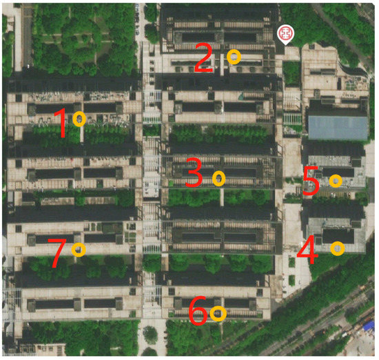
Figure 4.
Sensor geographical layout area, the yellow circles represent the sensors.
In this paper, we assumed that distributed generation had power supply points at the installation location of each PV sensor, and the area of the photovoltaic power panel at each power generation point was 10 m2. The relationship between solar irradiance and photovoltaic power generation is given by the following formula:
where, W represents the power generation per unit area, the unit is W/m2, J represents the light intensity per unit area, J/m2, and E is the conversion coefficient, which is related to the performance of the photovoltaic power panel.
3.2. Experimental Background Information
Our experiment was run on a PC and its compatible computers, using Windows operating system, the program code was written based on python version 3.7.1 and torch1.10.1, and the program running software was pycharm.
3.3. Data Preprocessing
For ROLL-GNN, BP, and LSTM, the power data of the real dataset were normalized in the same way: the data of each node were normalized according to the maximum power generation in the training year. The resolution of the data was 1 s.
3.4. Evaluation and Metrics
The proposed model and benchmark methods were compared on real datasets. Both the peak normalized mean square error (MSE) and the mean absolute percentage error (MAPE) were used as metrics. They are defined as follows:
where P1(t) is the predicted value of power generation at time t, P(t) is the true value of power generation at time t, and T is the length of the evaluation time.
3.5. Training
The ratio of the training dataset, validation dataset, and test dataset of our model was 7:1:2. All datasets were first randomly shuffled according to the number of days, and then allocated to the training dataset, validation dataset, and test dataset, in proportion. The specific parameters of the model are shown in Table 1.

Table 1.
Model parameter table.
3.6. Baselines
The BP neural network and the LSTM prediction model were used as the benchmark of distributed photovoltaic power generation prediction evaluation. BP has an excellent nonlinear mapping capability, and LSTM has a long-term memory function, which is suitable for long-term timeseries prediction. BP neural network and LSTM prediction models are typical models which are popular in various prediction scenarios, so they were selected as benchmark models in this paper.
4. Results and Discussion
We first predicted the total electricity in the distributed generation area for 60 s, 180 s, and 300 s in advance in the whole dataset, and evaluated the performance of the prediction results with the two indicators, MSE and MAPE. Table 2 shows the experimental results of the MAPE of the three algorithms in the overall dataset at 60 s, 180 s, and 300 s in advance.
Table 2.
Forecasting performance on the whole dataset.
The results show that, on the overall dataset, ROLL-GNN was superior to the other two methods in the two prediction modes of 60 s and 180 s in advance, which indicates that ROLL-GNN has a stronger fitting effect than BP and LSTM in these two modes and shows the effectiveness of ROLL-GNN in capturing the cloud dynamics from photovoltaic production data. This result comes from the establishment of the mathematical model of correlation analysis, which can obtain the cloud movement information in a specified period and provides the adjacency matrix based on spatio-temporal correlation for the graph neural network. These adjacency matrices determine the information flow direction of each node in the distributed generation prediction. However, in the prediction mode of 300 s in advance, the prediction accuracy of ROLL-GNN was almost the same as that of the BP neural network, which indicates that the ability of ROLL-GNN to capture the spatio-temporal correlation of PV power production data began to decline, because the distance between PV sensors was too close, which led to the decline of the accuracy of the mathematical model of the correlation analysis. The principle here is that there is a maximum time limit for the cloud to move in the area of the PV sensor, and upon approaching this limit, the cloud movement pattern will change. This limit is determined by the speed at which the cloud moves and the radius of the area where the sensor is placed.
In order to verify the advanced perception ability of the ROLL-GNN model in the face of volatility, we selected two days with different data types (smooth and multi-volatility) in the test set and analyzed the prediction results of these two days in detail. The MSE and MAPE of the corresponding data are shown in Table 3 and Table 4.
Table 3.
Forecasting performance on the smooth dataset.
Table 4.
Forecasting performance on the multi-volatility dataset.
The above results show that the prediction accuracy of ROLL-GNN was better than that of BP and LSTM in both datasets with smooth data and more fluctuating data, which indicates the effectiveness of ROLL-GN’s ability to sense the fluctuation of photovoltaic production data in advance in both datasets. We first screened out obvious fluctuations (as shown in Figure 5 and Figure 6) from the prediction results of the model predicted 60 s in advance for analysis.
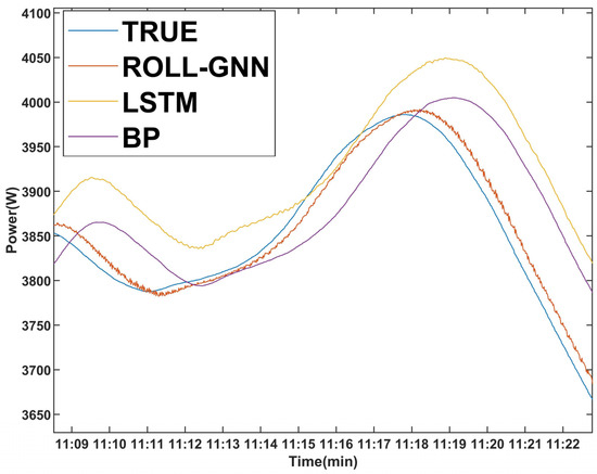
Figure 5.
Power generation prediction results (60 s in advance, smooth dataset).
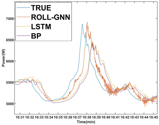
Figure 6.
Power generation prediction results (60 s in advance, multi-volatility dataset).
Figure 5 shows the prediction mode of 60 s in advance. For the smooth dataset, the real power generation value of the attachment had a large decline at 11:18:00, the predicted value of BP and LSTM algorithms had a large decline at 11:19:00, and the prediction result of the ROLL-GNN model had a large decline at 11:18:30. Figure 6 also shows the prediction mode of 60 s in advance. For the dataset with more fluctuations, the real power generation value of the attachment greatly decreased at 10:37:30, and the predicted value of BP and LSTM algorithms began to greatly decrease at 10:38:30. The prediction results of the ROLL-GNN model showed a large decline at 10:38:00, which indicates the effectiveness of the ROLL-GNN model in capturing the spatio-temporal correlation and advance perception of PV production data in the prediction mode of 60 s in advance. The prediction results of the 180 s in advance prediction mode were screened for obvious fluctuations, as shown in Figure 7 and Figure 8.
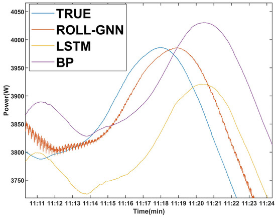
Figure 7.
Power generation prediction results (180 s in advance, smooth dataset).
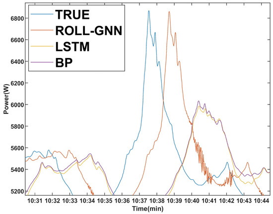
Figure 8.
Power generation prediction results (180 s in advance, multi-volatility dataset).
Figure 7 shows the prediction mode of 180 s in advance. For the smooth dataset, the real power generation value of the attachment had a large decline at 11:18:00, the predicted value of the BP and LSTM algorithms had a large decline at 11:21:00, and the prediction result of the ROLL-GNN model had a large decline at 10:19:10. Figure 8 also shows the prediction mode of 180 s in advance. The dataset had more fluctuations, the real power generation value of the attachment greatly decreased at 10:37:30, and the predicted value of the BP and LSTM algorithms began to greatly decrease at 10:41:00. The prediction results of the ROLL-GNN model showed a large decrease at 10:38:45, which indicates the effectiveness of the ROLL-GNN model in capturing the spatio-temporal correlation and advance perception of PV production data in the mode predicted 180 s in advance. The prediction results of the 300 s in advance prediction mode were screened for obvious fluctuations, as shown in Figure 9 and Figure 10.
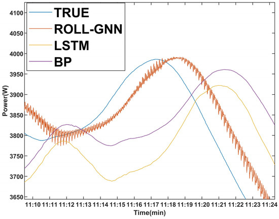
Figure 9.
Power generation prediction results (300 s in advance, smooth dataset).
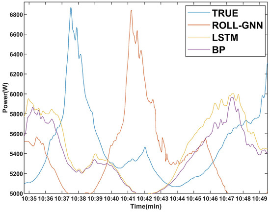
Figure 10.
Power generation prediction results (300 s in advance, multi-volatility dataset).
It can be seen from Figure 9 that in the prediction mode of 300 s in advance, for the smooth dataset, the real power generation value of the attachment had a large decline at 11:18:00, the predicted value of the BP and LSTM algorithms had a large decline at 11:22:00, and the prediction result of the ROLL-GNN model had a large decline at 10:20:00. It can be seen from Figure 10 that in the prediction mode of 300 s in advance, for the dataset with more fluctuations, the real power generation value of the attachment greatly decreased at 10:37:30. The fitting effect of the predicted value and the real value of the BP and LSTM algorithms was poor, and no similar waveform could be seen. The prediction results of the ROLL-GNN model showed a large decline at 10:41:05, which indicates that in the prediction mode of 300 s in advance, for the data with smooth data features, the ROLL-GNN model captured the spatio-temporal correlation and the effectiveness of advanced perception of photovoltaic production data, and for the data with more fluctuating data features, the ROLL-GNN model can also capture the spatio-temporal correlation of photovoltaic production data and the effectiveness of advanced perception. The advanced perception of ROLL-GNN decreased.
Whether it is a smooth dataset or a dataset with many fluctuations, the degree of fit between the predicted curve and the true value curve of ROLL-GNN was better than that of BP and LSTM. This was seen in two aspects. On the one hand, on sunny days, BP, LSTM, and ROLL-GNN had similar followability to the real data. In the face of PV output fluctuations, most segments of BP- and LSTM-predicted values did not have beating segments similar to the real data. Unlike BP and LSTM, when facing PV output fluctuations, the predicted value of ROLL-GNN had a high similarity with the fluctuation segments of real data. This indicates that the information between PV generation units in distributed generation is transferred to each other through ROLL-GNN, which can improve the accuracy of the prediction. On the other hand, whether in sunny or cloudy weather, ROLL-GNN had a more advanced perception ability than BP and LSTM in the face of a sudden big jump or big lift. The results showed that the prediction curve of ROLL-GNN was closer to the real value curve in the time axis in the face of a sudden big jump or big lift. This shows that the generation point of distributed generation can effectively use the information of other generation points. When the data of other PV generation points changed, such as with a large jump, the target PV generation point could sense the change in advance, which led to the advanced perception ability of ROLL-GNN. This advanced perception ability was realized by the graph neural network in the model.
The ROLL-GNN model proposed in this paper can not only improve the schedule of distributed PV generation prediction but can also make the distributed prediction have an advanced perception ability, which improved the grid’s dispatch ability in the face of sharp changes in the distributed PV power generation. The dispatch department of the grid can dispatch and understand the changes and adopt the frequency modulation measures in advance. Advance sensing helps to quickly start up the reserve capacity and avoid grid collapse.
5. Conclusions
This paper introduced a new graph convolutional neural network architecture for distributed photovoltaic power generation prediction, ROLL-GNN. This work used real data with a resolution of one second to compare ROLL-GNN with BP neural network and LSTM algorithms in three prediction intervals, i.e., 60, 180, and 300 s in advance. The comparison of the experimental results showed that for the test set of the whole dataset, the mean absolute percentage error (MAPE) of ROLL-GNN prediction results in the prediction mode of 60 s in advance was 1.72%, which is 4.01% less than that of the BP neural network and 1.1% less than that of the LSTM algorithm. In the prediction mode of 180 s in advance, the MAPE of ROLL-GNN prediction results was 4.65%, which is 1.59% less than that of the BP neural network and 3.86% less than that of the LSTM algorithm. In the prediction mode 300 s in advance, the MAPE of the prediction results of ROLL-GNN was 7.86%, which is 0.12% less than that of the BP neural network and 2.93% less than that of the LSTM algorithm.
By our estimation, an overly long advanced prediction time will decrease the accuracy. As the accuracy improvement was due to extra irradiance fluctuation information from neighboring PV panels or sensors, ‘how to advance the neighboring information to the target PV panel’ is the critical factor influencing the accuracy in different advance times. For example, if a cloud is coming towards the target panel from the east and there is a neighboring panel located at 200 m east of the target panel, and the wind speed at the cloud level is 2 m/s, then the neighboring panel can obtain about 200/2 = 100 s advance information to the target panel. If the prediction on the target panel is then changed to 5 min, this neighboring panel will lose its usage. In summary, a longer advanced prediction time requires a further neighboring panel to support its accuracy.
Through the similarity analysis of historical data, ROLL-GNN obtains the law of cloud dynamic influence on distributed power generation, which enables ROLL-GNN to have an advanced sensing ability, especially when the distributed PV power generation suddenly drops in a short period of time. Facing the sudden drop in power generation, the grid needs to prepare sufficient spare generation capacity. The benefit of ROLL-GNN is that in the face of the sharp changes of distributed photovoltaic power generation, the grid dispatch department can perceive the sharp change of electricity in advance through the ROLL-GNNY prediction model, and take frequency regulation measures in advance, which can reduce the cost of the power grid to the reserve capacity.
However, one of the limitations for ROLL-GNN is that it takes a long time for the ROLL-GNN model to perform the training calculation. Moreover, because the influence of cloud movement on photovoltaic power generation is related to the distance between the distributed photovoltaic power generation points, the prediction effect will become worse when the distance between the distributed photovoltaic power generation points is small and the advanced prediction time is long. We will further study the influence of distance on the advanced perception of ROLL-GNN in future works.
Author Contributions
J.X.: Supervision, Methodology, Investigation, and Software. Z.K.: Conceptualization, Software, and Formal Analysis. C.S.L.: Validation Writing—Review and Editing. Y.W.: Software and Validation. F.X.: Supervision, Project Administration, and Mathematical Modeling. H.Y.: Code Debugging, Visualization, and Formal Analysis. All authors have read and agreed to the published version of the manuscript.
Funding
This research was supported in part by Guangdong Basic and Applied Basic Research Foundation (2021A1515010742, 2020A1515011160, 2020A1515010801), in part by National Natural Science Foundation of China (52007032), in part by Basic Research Program of Jiangsu Province (BK20200385).
Institutional Review Board Statement
Not applicable.
Informed Consent Statement
Not applicable.
Data Availability Statement
The data presented in this study are available on request from the corresponding author.
Conflicts of Interest
The authors declare no conflict of interest.
References
- Chaturvedi, D.K.; Isha, I. Solar power forecasting: A review. Int. J. Comput. Appl. 2016, 145, 28–50. [Google Scholar]
- Wu, Y.K.; Chen, C.R.; Abdul Rahman, H. A novel hybrid model for short-term forecasting in PV power generation. Int. J. Photoenergy 2014, 2014, 569249. [Google Scholar] [CrossRef]
- Wang, Z.; Guo, Y.; Wang, H. Review on Monitoring and Operation-Maintenance Technology of Far-Reaching Sea Smart Wind Farms. J. Mar. Sci. Eng. 2022, 10, 820. [Google Scholar] [CrossRef]
- Kou, L.; Li, Y.; Zhang, F.; Gong, X.; Hu, Y.; Yuan, Q.; Ke, W. Review on Monitoring, Operation and Maintenance of Smart Offshore Wind Farms. Sensors 2022, 22, 2822. [Google Scholar] [CrossRef] [PubMed]
- Wang, H.; Ge, L.; Li, H.; Chi, F. A review on characteristic analysis and prediction method of distributed PV. Electr. Power Constr. 2017, 38, 1–9. [Google Scholar]
- Tan, J.; Deng, C.; Yang, W.; Liang, N.; Li, F. Ultra-short-term photovoltaic power forecasting in microgrid based on adaboost clustering. Autom. Electr. Power Syst. 2017, 41, 33–39. [Google Scholar]
- Antonanzas, J.; Osorio, N.; Escobar, R.; Urraca, R.; Martinez-De-Pison, F.J.; Antonanzas-Torres, F. Review of photovoltaic power forecasting. Sol. Energy 2016, 136, 78–111. [Google Scholar] [CrossRef]
- Huang, J.; Perry, M. A semi-empirical approach using gradient boosting and k-nearest neighbors regression for GEFCom2014 probabilistic solar power forecasting. Int. J. Forecast. 2016, 32, 1081–1086. [Google Scholar] [CrossRef]
- Li, Z.; Rahman, S.M.; Vega, R.; Dong, B. A hierarchical approach using machine learning methods in solar photovoltaic energy production forecasting. Energies 2016, 9, 55. [Google Scholar] [CrossRef]
- Sperati, S.; Alessandrini, S.; Delle Monache, L. An application of the ECMWF Ensemble Prediction System for short-term solar power forecasting. Sol. Energy 2016, 133, 437–450. [Google Scholar] [CrossRef]
- Pierro, M.; De Felice, M.; Maggioni, E.; Moser, D.; Perotto, A.; Spada, F.; Cornaro, C. A new approach for regional photovoltaic power estimation and forecast. In Proceedings of the 33rd European Photovoltaic Solar Energy Conference and Exhibition (EUPVSEC), Amsterdam, The Netherlands, 25–29 September 2017. [Google Scholar]
- Chu, Y.; Urquhart, B.; Gohari, S.M.; Pedro, H.T.; Kleissl, J.; Coimbra, C.F. Short-term reforecasting of power output from a 48 MWe solar PV plant. Sol. Energy 2015, 112, 68–77. [Google Scholar] [CrossRef]
- Jang, H.S.; Bae, K.Y.; Park, H.S.; Sung, D.K. Solar power prediction based on satellite images and support vector machine. IEEE Trans. Sustain. Energy 2016, 7, 1255–1263. [Google Scholar] [CrossRef]
- Schmidt, T.; Calais, M.; Roy, E.; Burton, A.; Heinemann, D.; Kilper, T.; Carter, C. Short-term solar forecasting based on sky images to enable higher PV generation in remote electricity networks. Renew. Energy Environ. Sustain. 2017, 2, 23. [Google Scholar] [CrossRef]
- Hu, K.; Cao, S.; Wang, L.; Li, W.; Lv, M. A new ultra-short-term photovoltaic power prediction model based on ground-based cloud images. J. Clean. Prod. 2018, 200, 731–745. [Google Scholar] [CrossRef]
- Geraldi, E.; Romano, F.; Ricciardelli, E. An advanced model for the estimation of the surface solar irradiance under all atmospheric conditions using MSG/SEVIRI data. IEEE Trans. Geosci. Remote Sens. 2012, 50, 2934–2953. [Google Scholar] [CrossRef]
- Wang, F.; Xuan, Z.; Zhen, Z.; Li, K.; Wang, T.; Shi, M. A day-ahead PV power forecasting method based on LSTM-RNN model and time correlation modification under partial daily pattern prediction framework. Energy Convers. Manag. 2020, 212, 112766. [Google Scholar] [CrossRef]
- Wang, L.; Mao, M.; Xie, J.; Liao, Z.; Zhang, H.; Li, H. Accurate solar PV power prediction interval method based on frequency-domain decomposition and LSTM model. Energy 2023, 262, 125592. [Google Scholar] [CrossRef]
- Kleissl, J.; Bosch, J.L.; Kurtz, B.; Lave, M.; Lopez, I.; Mathiesen, P.; Nguyen, A.; Urquhart, B. Recent Advances in Solar Variability Modeling and Solar Forecasting at UC San Diego. In Proceedings of the American Solar Energy Society, 2013 Solar Conference, Baltimore, MD, USA, 16–20 April 2013. [Google Scholar]
- McCandless, T.C.; Haupt, S.E.; Young, G.S. A model tree approach to forecasting solar irradiance variability. Sol. Energy 2015, 120, 514–524. [Google Scholar] [CrossRef]
- Monjoly, S.; André, M.; Calif, R.; Soubdhan, T. Forecast horizon and solar variability influences on the performances of multiscale hybrid forecast model. Energies 2019, 12, 2264. [Google Scholar] [CrossRef]
- Wang, F.; Xuan, Z.; Zhen, Z.; Li, Y.; Li, K.; Zhao, L.; Shafie-khah, M.; Catalão, J.P. A minutely solar irradiance forecasting method based on real-time sky image-irradiance mapping model. Energy Convers. Manag. 2020, 220, 113075. [Google Scholar] [CrossRef]
- Lappalainen, K.; Valkealahti, S. Output power variation of different PV array configurations during irradiance transitions caused by moving clouds. Appl. Energy 2017, 190, 902–910. [Google Scholar] [CrossRef]
- Liu, X.; Wang, J.; Yao, T.; Zhang, P.; Chi, X. Ultra Short Term Distributed Photovoltaic Power Prediction Based on Satellite Remote Sensing. Trans. China Electrotech. Soc. 2022, 31, 1800–1809. [Google Scholar]
- Guanjun, B.; Liubin, T.; Shibo, C.; Jianjun, T.; Linwei, Z.; Fang, X. An ultra-short-term power prediction model based on machine vision for distributed photovoltaic system. In Proceedings of the 2015 IEEE International Conference on Information and Automation, Lijiang, China, 8–10 August 2015; pp. 1148–1152. [Google Scholar]
- Simeunovic, J.; Schubnel, B.; Alet, P.-J.; Carrillo, R.E. Spatio-temporal graph neural networks for multi-site PV power forecasting. IEEE Trans. Sustain. Energy 2021, 13, 1210–1220. [Google Scholar] [CrossRef]
- Tiwari, S.; Sabzehgar, R.; Rasouli, M. Short term solar irradiance forecast based on image processing and cloud motion detection. In Proceedings of the 2019 IEEE Texas Power and Energy Conference (TPEC), College Station, TX, USA, 7–8 February 2019; pp. 1–6. [Google Scholar]
- Kong, W.; Jia, Y.; Dong, Z.Y.; Meng, K.; Chai, S. Hybrid approaches based on deep whole-sky-image learning to photovoltaic generation forecasting. Appl. Energy 2020, 280, 115875. [Google Scholar] [CrossRef]
- Pothineni, D.; Oswald, M.R.; Poland, J.; Pollefeys, M. Kloudnet: Deep learning for sky image analysis and irradiance forecasting. In Proceedings of the Pattern Recognition: 40th German Conference, GCPR 2018, Stuttgart, Germany, 9–12 October 2018; Proceedings 40. Springer International Publishing: Berlin/Heidelberg, Germany, 2019; pp. 535–551. [Google Scholar]
- Xu, X.; Niu, D.; Wang, Q.; Wang, P.; Wu, D.D. Intelligent forecasting model for regional power grid with distributed generation. IEEE Syst. J. 2015, 11, 1836–1845. [Google Scholar] [CrossRef]
- Changsong, C.; Shanxu, D.; Jinjun, Y. Research of energy management system of distributed generation based on power forecasting. In Proceedings of the 2008 International Conference on Electrical Machines and Systems, Wuhan, China, 17–20 October 2008; pp. 2734–2737. [Google Scholar]
- Agoua, X.G.; Girard, R.; Kariniotakis, G. Short-term spatio-temporal forecasting of photovoltaic power production. IEEE Trans. Sustain. Energy 2017, 9, 538–546. [Google Scholar] [CrossRef]
- Yang, C.; Thatte, A.A.; Xie, L. Multitime-scale data-driven spatio-temporal forecast of photovoltaic generation. IEEE Trans. Sustain. Energy 2014, 6, 104–112. [Google Scholar] [CrossRef]
- Chai, S.; Xu, Z.; Jia, Y.; Wong, W.K. A robust spatiotemporal forecasting framework for photovoltaic generation. IEEE Trans. Smart Grid 2020, 11, 5370–5382. [Google Scholar] [CrossRef]
- Jeong, J.; Kim, H. Multi-site photovoltaic forecasting exploiting spacetime convolutional neural network. Energies 2019, 12, 4490. [Google Scholar] [CrossRef]
- Zhu, Q.; Chen, J.; Zhu, L.; Duan, X.; Liu, Y. Wind speed prediction with spatio–temporal correlation: A deep learning approach. Energies 2018, 11, 705. [Google Scholar] [CrossRef]
- Zhang, C.; Peng, T.; Nazir, M.S. A novel integrated photovoltaic power forecasting model based on variational mode decomposition and CNN-BiGRU considering meteorological variables. Electr. Power Syst. Res. 2022, 213, 108796. [Google Scholar] [CrossRef]
- Zhou, H.; Zhang, Y.; Yang, L.; Liu, Q.; Yan, K.; Du, Y. Short-term photovoltaic power forecasting based on long short term memory neural network and attention mechanism. IEEE Access 2019, 7, 78063–78074. [Google Scholar] [CrossRef]
- Shih, S.-Y.; Sun, F.-K.; Lee, H.-Y. Temporal pattern attention for multivariate time series forecasting. Mach. Learn. 2019, 108, 1421–1441. [Google Scholar] [CrossRef]
- Ortega, A.; Frossard, P.; Kovăcevi’c, J.; Moura, J.M.F.; Vandergheynst, P. Graph signal processing: Overview, challenges, and applications. Proc. IEEE 2018, 106, 808–828. [Google Scholar] [CrossRef]
- Zhou, J.; Cui, G.; Hu, S.; Zhang, Z.; Yang, C.; Liu, Z.; Wang, L.; Li, C.; Sun, M. Graph neural networks: A. review of methods and applications. AI Open 2020, 1, 57–81. [Google Scholar] [CrossRef]
- Wu, Z.; Pan, S.; Chen, F.; Long, G.; Zhang, C.; Yu, P. A comprehensive survey on graph neural networks. IEEE Trans. Neural Netw. Learn. Syst. 2021, 32, 4–24. [Google Scholar] [CrossRef]
- Zhang, R.; Ma, H.; Hua, W.; Saha, T.K.; Zhou, X. Data-driven photovoltaic generation forecasting based on a Bayesian network with spatial–temporal correlation analysis. IEEE Trans. Ind. Inform. 2019, 16, 1635–1644. [Google Scholar] [CrossRef]
- Lai, C.S.; Tao, Y.; Xu, F.; Ng, W.W.; Jia, Y.; Yuan, H.; Huang, C.; Lai, L.L.; Xu, Z.; Locatelli, G. A robust correlation analysis framework for imbalanced and dichotomous data with uncertainty. Inf. Sci. 2019, 470, 58–77. [Google Scholar] [CrossRef]
- Chaudhary, P.; Rizwan, M. Short term solar energy forecasting using GNN integrated wavelet-based approach. Int. J. Renew. Energy Technol. 2019, 10, 229–246. [Google Scholar] [CrossRef]
- Chaturvedi, D.K. Forecasting of solar power using quantum ga-gnn. Int. J. Comput. Appl. 2015, 975, 8887. [Google Scholar] [CrossRef]
- Wu, D.; Lin, W. Efficient residential electric load forecasting via transfer learning and graph neural networks. IEEE Trans. Smart Grid 2022, 14, 2423–2431. [Google Scholar] [CrossRef]
- Zhang, D.; Ren, Z.; Bi, Y.; Zhou, D.; Bi, Y. Power load forecasting based on grey neural network. In Proceedings of the 2008 IEEE International Symposium on Industrial Electronics, Cambridge, UK, 30 June–2 July 2008; pp. 1885–1889. [Google Scholar]
- Chaudhary, P.; Rizwan, M. Short-term PV power forecasting using generalized neural network and weather-type classification. In Advances in Energy and Power Systems: Select Proceedings of ICAEDC 2017; Springer: Singapore, 2018; pp. 13–20. [Google Scholar]
- Karimi, A.M.; Wu, Y.; Koyuturk, M.; French, R.H. Spatiotemporal graph neural network for performance prediction of photovoltaic power systems. In Proceedings of the AAAI Conference on Artificial Intelligence, Virtually, 2–9 February 2021; Volume 35, pp. 15323–15330. [Google Scholar]
- Chaturvedi, D.K.; Premdayal, S.A.; Chandiok, A. Short-term load forecasting using soft computing techniques. Int. J. Commun. Netw. Syst. Sci. 2010, 3, 273. [Google Scholar] [CrossRef]


Disclaimer/Publisher’s Note: The statements, opinions and data contained in all publications are solely those of the individual author(s) and contributor(s) and not of MDPI and/or the editor(s). MDPI and/or the editor(s) disclaim responsibility for any injury to people or property resulting from any ideas, methods, instructions or products referred to in the content. |
© 2023 by the authors. Licensee MDPI, Basel, Switzerland. This article is an open access article distributed under the terms and conditions of the Creative Commons Attribution (CC BY) license (https://creativecommons.org/licenses/by/4.0/).