This section contains three case studies that showcase the advantages of the presented method under different operating conditions and constraints. Each case study includes key performance metrics as well as comparisons with other methods found in literature. Before proceeding to the test cases, an illustrative example is presented. The purpose of the example is to summarize the topics and steps discussed in the previous sections.
5.1. Illustrative Example
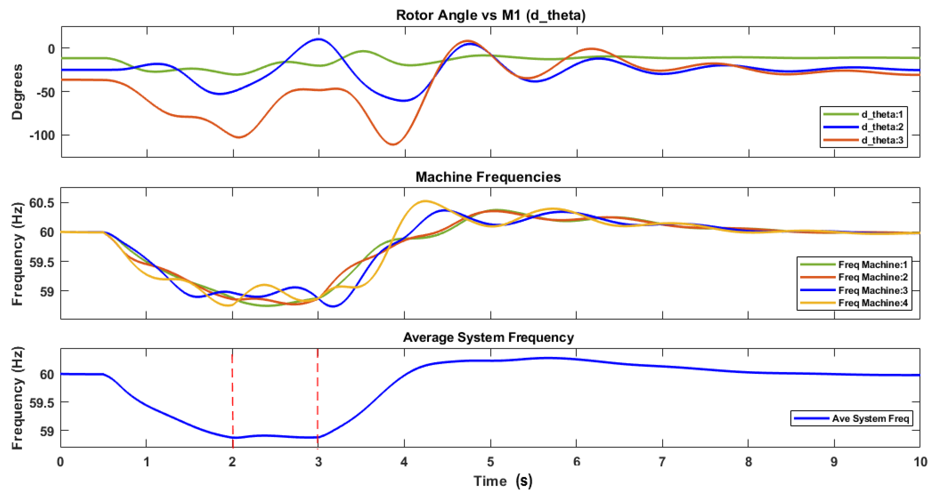
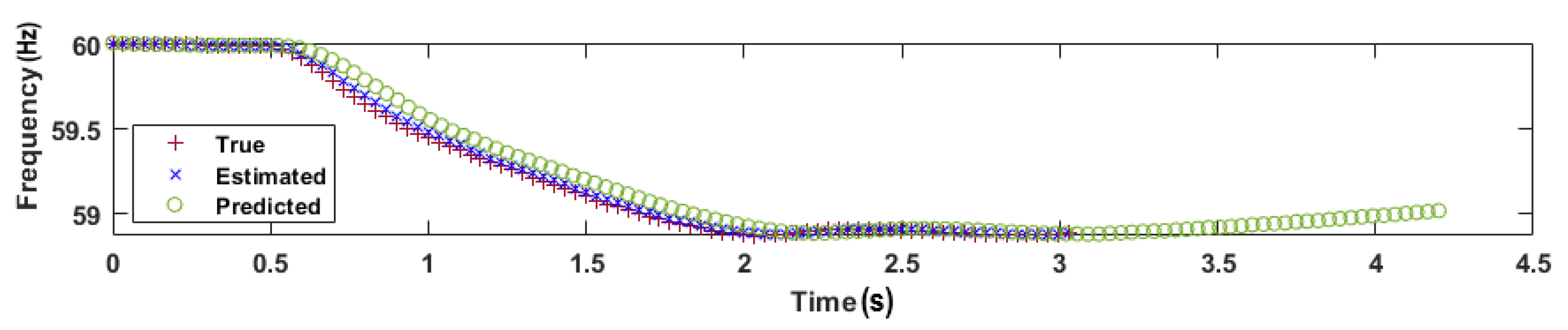
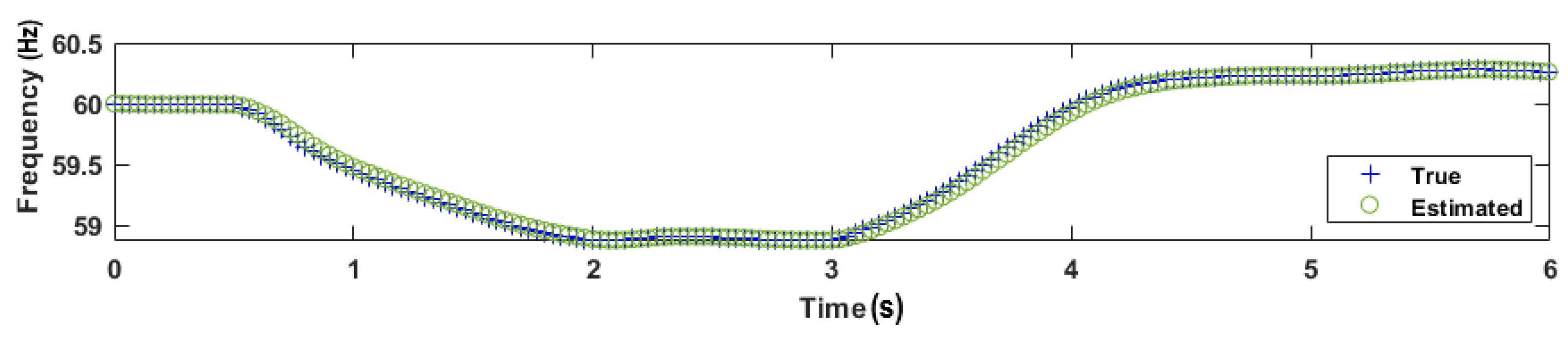
Figure 7 illustrates the complete response of a four-machine system after a disturbance is introduced and mitigated using the scheme presented in this work.
The disturbance starts at 0.5 s, and it is detected via the RoCoF from Equation (
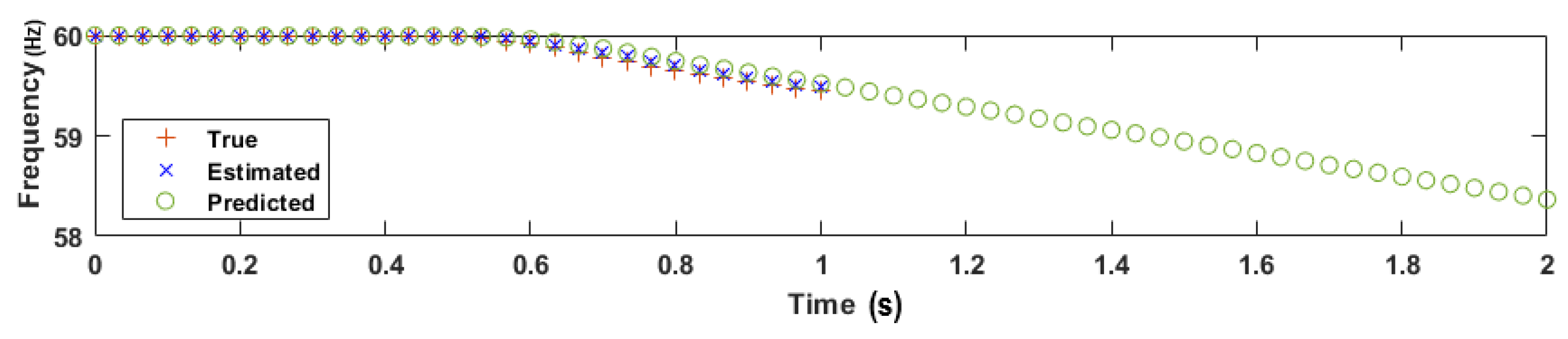
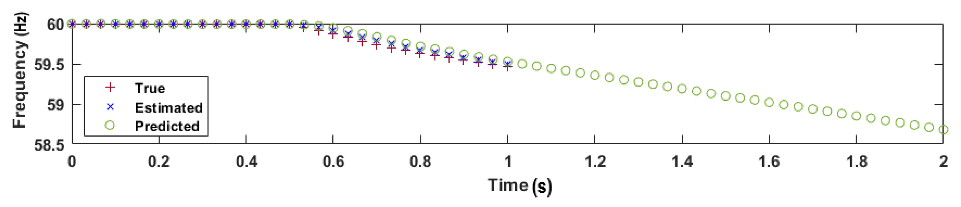
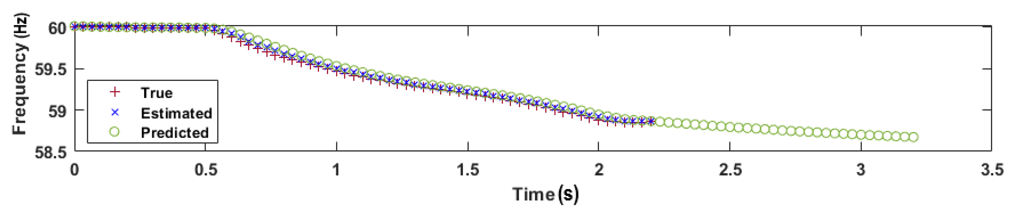
4). At 1 s, a prediction is made as shown in
Figure 8. Dotted vertical lines in red, considering
Figure 7, represent compensation stages derived with the solution. To account for processing and communication delays, corrective actions are taken one full second after a prediction is made.
The method estimates the state of the system frequency one second into the future. These estimates are then used to calculate the loading excess via Equation (
8), which is then followed by a compensation stage at 2 s, as seen in
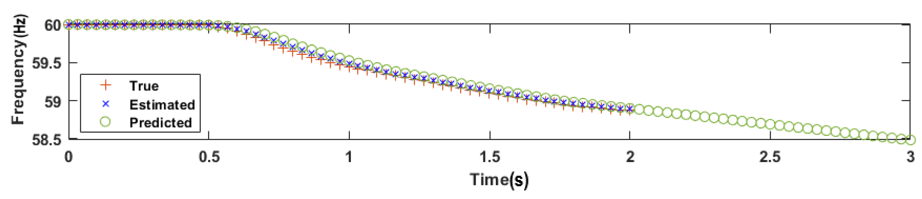
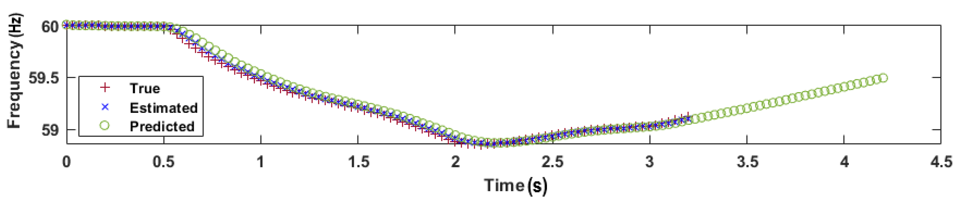
Figure 7. A second prediction is made immediately after the first stage of compensation, this is shown in
Figure 9.
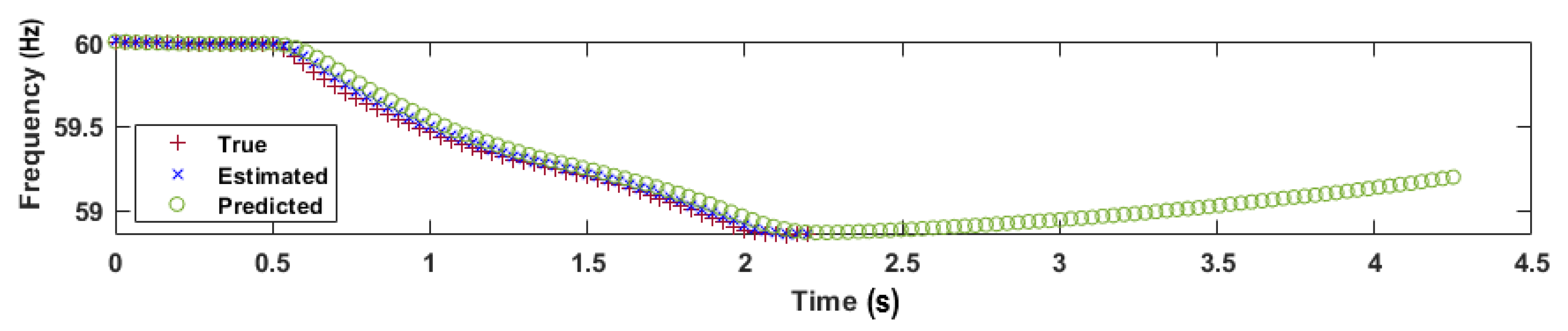
Based on this new prediction, a second stage of compensation is executed at 3 s, which is then followed by a third prediction as illustrated in
Figure 10.
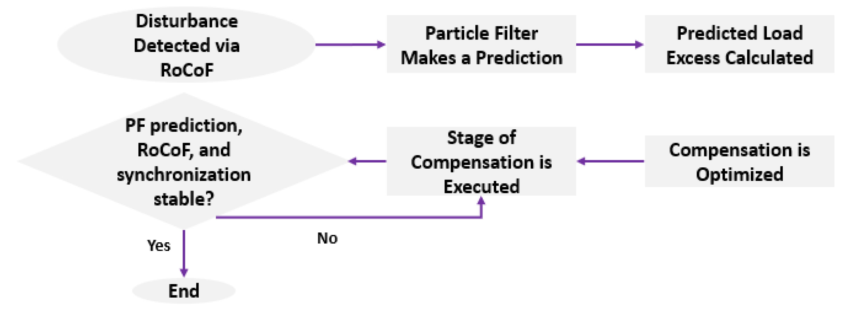
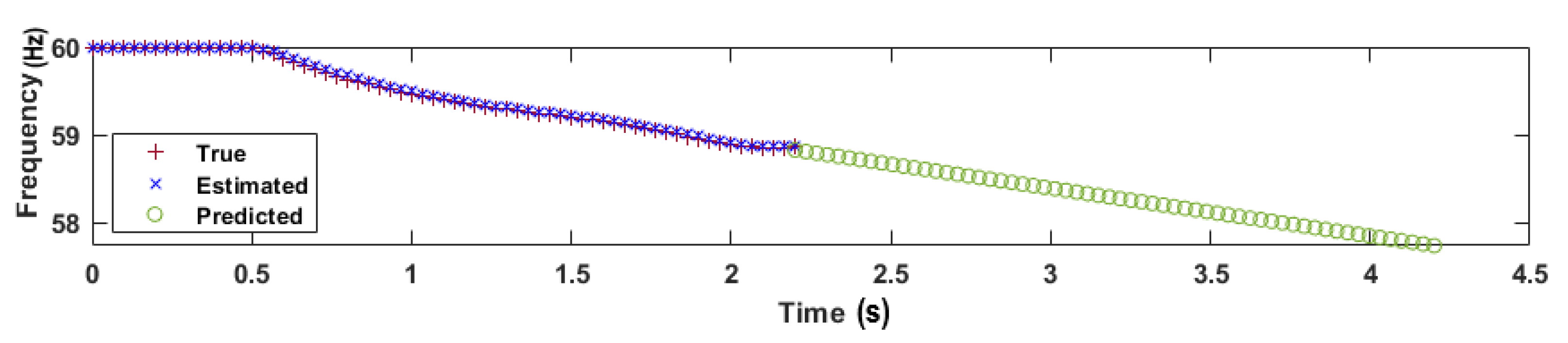
The third prediction shows that the frequency is trending back into stability. Since frequency is expected to return to its normal range, a third stage of compensation is not executed. In this case the system regains stability with minimal overshoot as seen in
Figure 11.
Subsequent stages of compensation are not executed when three conditions are met:
The goal of the method is to first stop the decay in frequency, and second, to send it back to a range where generator governors can stabilize it.
5.2. Case Study I
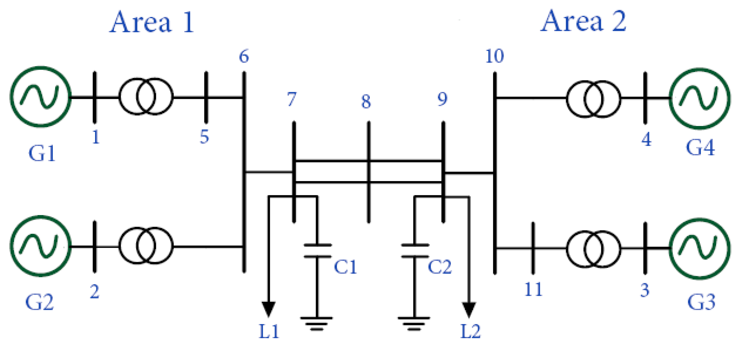
This case study contains four scenarios and it is based on Kundur’s Two-Area System. This model can be found at [
46]. The locations where excesses in load are introduced are numbered (1 through 4) in
Figure 12. Loading, capacity, and other operational parameters are presented in
Table 1 and
Table 2, and also in
Table A1 in the
Appendix A. Considering
Figure 12, buses are referred by numbers, loads by the letter ‘L’ followed by a number, capacitor banks by the letter ‘C’ followed by a number, and generators by the letter ‘G’ followed by a number. Again, to account for processing and communication delays, corrective actions are taken one full second after a prediction is made. Gaussian noise with a variance of 0.025 is added to the measurements.
The scenario where the load excess is placed at bus 1 in
Figure 12, is run twice. First, a fixed three stage compensation procedure is used. The first compensation stage is set at 50% of the calculated load excess. Stages 2 and 3 compensate 25% of the load excess each, for a total of 100%, similar to the approach used by [
7]. The load imbalance starts at 0.5 s, and each compensation stage is illustrated through vertical dotted red lines in
Figure 13.
In this case the system was successful in first, arresting the decline in frequency, and second, in providing a smooth transition back to steady state. Three predictions were made by the particle filter, they are presented in
Figure 14,
Figure 15 and
Figure 16:
This same scenario was performed using a version of the algorithm referred to as adaptive compensation. Adaptive compensation works as follows: The initial stage compensates for 50% of the estimated excess load factor. After the first stage is executed, the number of samples used in obtaining the derivatives in Equation (
5) is decreased, making the particle filter more receptive to system dynamics. Compensation with variable stages is illustrated in
Figure 17 through a red dotted vertical line.
In this case, the PF predicts that frequency will be returning to levels close to the reference after only one stage of compensation. This is shown in
Figure 18.
With frequency expected to return to its normal range, and
not trending towards loss of synchronism, further compensation stages are avoided. Being able to restore frequency stability while compensating only a portion of the calculated load excess happens for two reasons: First, being able to take corrective actions early means that compensation can begin before the system reaches a critical state. Second, generator governors and other controllers are not considered during compensation calculations, and while this might lead to some inaccuracies, it also gives the scheme a safety margin, which translates into a lower amount of load shed. Realistically, a highly accurate load compensation value is difficult to obtain given the time constraints and the dynamics of both the loads and the sources. Moreover, it has been suggested that in the context of frequency stability, early action trumps accuracy [
7].
This scenario is performed once again with the adaptive compensation procedure, but this time, polynomial curve fitting (PCF) as presented in [
7], is used to obtain predictions instead of the PF. After the first stage of compensation has been executed, a follow up prediction is made as illustrated by
Figure 19.
The prediction obtained via polynomial curve fitting is unable to leverage the dynamics of the system the way the PF can, leading to further stages of compensation.
Three more disturbances are introduced and both the PF based method and the PCF technique are used to mitigate them. A performance comparison is presented in
Table 3.
For the four scenarios presented in
Table 3, the method presented in this paper was able to bring the system back into stability while shedding
to
less load. This is, as previously discussed, due to the ability of the prediction model to leverage the dynamics of the system as frequency begins to return to a stable condition. Performance metrics are examined in
Table 4, where frequency overshoot during recovery is measured.
As expected, more stages lead to a smoother transition back into steady state. It is worth noting that even when only one compensation stage was used, the overshoot was still fairly low.
5.3. Case Study II
A second case study was conducted using the IEEE 14-Bus System as reference. Following the same process as in the first case study, four scenarios are presented. The locations where the load excesses are introduced are presented in
Figure 20, through numbers. Loading, capacity, and other operational parameters are presented in
Table A2 in the
Appendix A.
Once again, each scenario is run twice, one time using PCF to build a base line and then using the PF. Key metrics are presented in
Table 5.
The results of this case study are consistent with the results of the first one, and they show that the PF based method facilitates the recovery of frequency while greatly reducing the amount of compensation used. Overshoot is also used as a performance metric for this case study, and the results are presented in
Table 6.
The observed overshoot in this scenario is once again fairly low, which is consistent with the results obtained in the first case study.
5.4. Case Study III
The goal of this final test case is to highlight the flexibility of the method and use it to drive distributed energy resources (DERs) in real-time. This test was run under a similar set of assumptions as those made in [
16], where a KF-based compensation method is presented. In order to test the algorithm under demanding conditions, faster frequency deviations than those seen in [
16] were generated. Most importantly, the total delay time involved in the processing of data and actuation of DERs was increased to 500 ms; up from the 40 ms time delay used in [
16]. That is a response time over ten times slower.
Frequency deviations start at 1 s, with a significant loss of generation at 1.5 s. As illustrated in
Figure 21, DER actuation takes place 0.5 s after the frequency deviations.
As before, measurements are made via PMUs at 30 fps. The power mismatch is calculated continuously in this test case per Equations (
4) and (
8) in the form of a controller. As shown in
Figure 21 above, the frequency and power mismatch follow virtually the same trend but in opposite directions. When frequency deviates from the 60 Hz reference, a corresponding current output is seen from the DERs. The compensation is based on the power mismatch calculated by the controller. Despite having a 0.5 s delay, the system successfully mitigates the frequency deviations.


