Modeling Annual Electricity Production and Levelized Cost of Energy from the US East Coast Offshore Wind Energy Lease Areas

Abstract

Offshore wind energy development along the East Coast of the US is proceeding quickly as a result of large areas with an excellent wind resource, low water depths and proximity to large electricity markets. Careful planning of wind turbine deployments in these offshore wind energy lease areas (LA) is required to maximize power output and to minimize wake losses between neighboring wind farms as well as those internal to each wind farm. Here, we used microscale wind modeling with two wake parameterizations to evaluate the potential annual energy production (AEP) and wake losses in the different LA areas, and we developed and applied a levelized cost of energy (LCoE) model to quantify the impact of different wind turbine layouts on LCoE. The modeling illustrated that if the current suite of LA is subject to deployment of 15 MW wind turbines at a spacing of 1.85 km, they will generate 4 to 4.6% of total national electricity demand. The LCoE ranged from $68 to $102/MWh depending on the precise layout selected, which is cost competitive with many other generation sources. The scale of the wind farms that will be deployed greatly exceed those currently operating and mean that wake-induced power losses are considerable but still relatively poorly constrained. AEP and LCoE exhibited significant dependence on the precise wake model applied. For the largest LA, the AEP differed by over 10% depending on the wake model used, leading to a $10/MWh difference in LCoE for the wind turbine layout with 1.85 km spacing.

1. Introduction

1.1. Offshore Wind Energy

Offshore wind energy is a critical component of many low-carbon energy portfolios designed to reduce carbon emissions while generating electricity at moderate cost [1]. The United States of America (US) is one of 46 countries that agreed to phase out coal at COP 26 and is pursuing the deployment of 30 GW of offshore wind energy by 2030 as part of this strategy [2]. Shallower coastal waters allowed an earlier expansion of offshore wind energy in Europe, where the first installations were in 1993 and installed capacity now exceeds 30 GW, including more than 100 MW of floating offshore wind turbine installed capacity [3,4]. The rated capacity of offshore wind turbines increased over 20 times from the 0.5 MW turbines installed in 1993 at Vindeby [5] to 13 MW (and larger) turbines planned for deployment off the US East Coast. Offshore wind turbine hub-heights increased from 37 m in 1991 to 100 m in 2021 and rotor diameters from 38 m to over 156 m [6].

In 2022, there were only seven wind turbines offshore in the US, and 16 offshore wind energy lease areas (LA) off the US East Coast were active, covering almost 7000 km² [7]. A further six LA in New York Bight (almost 2000 km²) were auctioned for a record $4.4 billion [8] in February 2022 (Figure 1 and

Table 1. Offshore lease areas (LA) for wind developments off the east coast of the USA. Information as provided by the US Bureau of Ocean Energy Management (BOEM), July 2022 [9]. The original 16 lease areas (auctioned prior to 2022) are shown in regular font [11], the lease areas that were auctioned in February 2022 are shown in italics.

LA Group	Project Name (Lessee)	Area (km2)	Identifier	Lease Date	Center Latitude (N)	Center Longitude (E)
MA	Sea2shore The Renewable Link	-	OCS-A 0506	2014	-	-
	Revolution Wind	339	OCS-A 0486	2013	41.16	−71.12
	South Fork Wind	55	OCS-A 0517	2013	41.10	−71.13
	Sunrise Wind	445	OCS-A 0487	2013	40.94	−71.08
	Bay State Wind	586	OCS-A 0500	2015	40.98	−70.84
	Vineyard Wind	264	OCS-A 0501	2015	41.11	−70.51
	New England Wind	411	OCS-A 0534	2015	40.95	−70.62
	Beacon Wind	521	OCS-A 0520	2018	40.84	−70.52
	(Mayflower)	516	OCS-A 0521	2019	40.75	−70.43
	Vineyard NE Wind	536	OCS-A 0522	2019	40.70	−70.20
NE	Empire Wind	321	OCS-A 0512	2017	40.27	−73.32
	(Mid-Atlantic Offshore Wind)	174	OCS-A 0544	2022	40.24	−73.08
	(OW Ocean Winds East)	289	OCS-A 0537	2022	39.95	−72.74
	(Attentive Energy)	341	OCS-A 0538	2022	39.71	−73.17
	(Bight Wind Holdings/Community Offshore Wind)	510	OCS-A 0539	2022	39.53	−73.32
	(Invenergy Wind Offshore)	340	OCS-A 0542	2022	39.31	−73.47
	(Atlantic Shores Offshore Wind Bight)	321	OCS-A 0541	2022	39.35	−73.60
NJ	Atlantic Shores North	328	OCS-A 0549	2016	39.50	−74.00
	Atlantic Shores South	413	OCS-A 0499	2016	39.30	−74.13
	Ocean Wind NJ	305	OCS-A 0498	2016	39.15	−74.20
	Ocean Wind 2	343	OCS-A 0532	2016	39.10	−74.42
	Garden State Offshore Energy I	284	OCS-A 0482	2012	38.60	−74.70
	Skipjack Wind Farm	107	OCS-A 0519	2018	38.56	−74.67
	MarWin	323	OCS-A 0490	2014	38.38	−74.78
VA	Coastal Virginia Offshore Wind Pilot	9	OCS-A 0497	2015	36.91	−75.50
	Coastal Virginia Offshore Wind	456	OCS-A 0483	2013	36.91	−75.36
	Kitty Hawk	496	OCS-A 0508	2017	36.34	−75.11

). There are now 30 active lease areas (LA) around the US, including one off the coast of Oregon and two to the south of North Carolina that are not included here [9]. Analyses of wind speeds at 100 m height from the ERA5 reanalysis data set [10] indicate that the original 16 LA along the US East Coast have mean wind speeds of 8.0–9.1 ms⁻¹ with highest wind speeds in the north [7]. The ERA5 data were used in the analyses presented here for consistency and because no measured data of hub-height wind speeds are available for all LA.

The centroids of these lease areas are 26–65 km from the coast, and the water depths are up to 70 m [7]. The most advanced projects are expected to begin production in 2023. These include Vineyard Wind I (south of Massachusetts, Table 1), which is anticipated to comprise 62 GE 13 MW Haliade-X turbines and South Fork I (east of Long Island) that is expected to comprise 12 Siemens-Gamesa 11 MW turbines. The remaining LA are at various stages of permitting and development (see BOEM.gov/renewable-energy accessed on 28 July 2022). Herein, the LA along the US east coast are grouped into four clusters that are geographically proximal (Table 1 and Figure 1). These groups are denoted using two letter identifiers: MA denotes the LA group south of Massachusetts and Rhode Island. NE indicates lease areas in the New York Bight and lie south of New York State and east of New Jersey. NJ denote the LA group east of New Jersey, Delaware and Maryland. VA indicates the lease areas east of Virginia.

1.2. Predicting Power Production: The Role of Wakes

The major components of a levelized cost of energy (LCoE) model for offshore wind energy are: capital expenditures, operating costs, discounting rate and the projected power output. This last factor was the focus of the research presented herein. Power production can be quoted in terms of the annual number of megawatt hours of electrical power produced (MWh/yr.) or in terms of the capacity factor. Capacity factors (CF, %) describe the amount of electrical power produced compared to that which would be produced, if all wind turbines ran consistently at their rated power, i.e., if all wind turbines generated the maximum amount of power that they are designed to produce at all times in a given year.

The power produced by a wind farm (i.e., cluster of wind turbines) is primarily determined by two factors: (i) the magnitude of the wind resource. In general wind speeds along the US east coast increase moving south to north [7] but are also dependent on the distance to shore [12]; (ii) the magnitude of wake-induced power losses due to individual wind turbines operating downwind of another turbine so in the wind ‘shadow’ caused by extraction of momentum from the atmosphere by the wind turbine rotor. The magnitude of the velocity deficit/power loss in the wake is strongly dependent on wind speed (via the wind turbine thrust coefficient) and the wind farm topology (turbine layout) [13]. This dictates interplay between the wind direction distribution and the effective wind turbine spacing and, thus, the downwind distance that the wake has to evolve and degrade before impacting an additional wind turbine. In wind farms with multiple rows and columns (here defined as turbine lines east–west and north–south, respectively), wakes merge downwind and from the sides. This leads to the ‘deep array effect’ with larger than anticipated power losses [14,15], because wake recovery is solely controlled by transport rates of higher momentum air from aloft downwards towards the rotor plane [16]. Wake losses tend to be larger offshore, mainly because ambient turbulence intensity is lower leading to low transport rates. Transport of momentum is also impacted by atmospheric stability and planetary boundary-layer heights (PBLH) (that are typically lower offshore) [17]. Merged wakes form whole-wind farm wakes that are characterized by wind speeds below the freestream encompassing large areas downwind of wind farms [18], which were measured offshore to over 17 km [19] and modelled extending over 12 km with large eddy simulations [20] and 90 km using the weather research and forecasting model [16].

For moderate sized offshore wind farms in Europe (installed capacities of up to 200 MW), wakes were shown to suppress total power output by 5–20% [21]. A direct relationship of 1–1.5% increase in total wind farm power generation efficiency for every 1 rotor diameter (1D) increase in wind turbine spacing (for 4–20 D) was found based on power production at two European offshore wind farms [22].

Determining optimal wind farm layouts, or the optimal distance between wind farms to reduce power losses due to wakes, requires detailed modeling of the turbine response to atmospheric conditions. Very few offshore wind farms have smaller turbine spacing than 3 D [23], but as spacing increases, both internal cable costs and the number of turbines that can be installed in given area decreases. The turbine spacing agreed in the Massachusetts/Rhode Island LA is on an east–west grid at 1 nautical mile (1.85 km), giving an installed capacity density (ICD) of 4.3 MW/km² if a 15 MW wind turbine [24] is selected. The ICD of European wind farms ranges averages 5.5–6.0 MW/km² ranging from 3 to 19 MW/km² [25]. There are several ways to define ICD in terms of which area to use (the minimum to extend over each turbine base or the total assigned area) in the definition. Here, we used the total area of the LA divided by the number of turbines, multiplied by the rated capacity of the wind turbine (the 15 MW IEA reference turbine was used in this study [24]).

There is a lack of available offshore wind speed observations to improve understanding of the wind resource and potential wake losses for the US east coast offshore wind energy lease areas [26]. Thus, in general, potential electricity generation for the US offshore wind farms is determined using simulations [16]. Mesoscale models such as the weather research and forecasting model (WRF) include sophisticated atmospheric physics and generate three-dimensional time-evolving fields of atmospheric variables at high resolution and was coupled to wind farm parameterizations [16,27] that use aerodynamic approximations to describe both power and wake generation, plus downstream wake dissipation. The wake parameterization is simplified [28] but is controlled by the turbine dimensions and wind speed dependent power and thrust coefficients.

A previous analysis using WRF and the Fitch wind farm parameterization [16] found that using a fixed turbine installed capacity density of 4.3 MW/km² in each of the original 16 lease areas (Table 1), the electrical production was 116 TWh/y or 3% of US total offshore wind electricity generation with a frequency-weighted CF of 45% and an average power loss due to wind turbine/wind farm wake losses of 35.3% [16]. For comparison, net CF, that include reductions in production due to transmission losses and losses due to maintenance activities in addition to wake effects, from operating offshore wind farms lie in the range of 38% to 42% [29,30,31]. Those WRF simulations [16] employed the International Energy Agency 15 MW reference wind turbine, which has a hub-height of 150 m and a rotor diameter of 240 m [24]. They also indicate that the wind farm wake (i.e., area covered by a velocity deficit of more than 5% of the undisturbed flow) can cover up to six times the area of the LA but is more typically two to four times that footprint. Sensitivity analyses showed both the CF and the wake extent are strongly dependent on (i) the freestream wind and turbulent kinetic energy; (ii) the wind direction which impacts both the effective wind turbine spacing and the stability related to directional air–sea temperature differences; and (iii) the turbine installed capacity density (ICD)/wind turbine spacing. For example, CF for the original 16 LA increases to 51.4% if the ICD is reduced to 2.2 MW/km² [16]. In addition to these dependencies on geophysical variables, both CF and wake extent are strongly influenced by treatment of the rotor aerodynamics (i.e., the wake parameterization). Under moderate wind speeds and turbulent kinetic energy (TKE), power output from the Fitch wind farm parameterization is 25% lower, and the wake extent is 18% larger than when an alternative formulation (EWP) is employed [18].

WRF is a good choice for simulating large-scale atmospheric variability and wake behavior, but WRF simulations are not suitable for internal array optimization, i.e., arranging the individual turbine positions, because the computational expense of WRF generally precludes its application at scales less than a few kilometers. Hence, turbine layouts are frequently optimized, as herein, using microscale models [32,33,34,35].

1.3. Levelized Cost of Energy Modeling

The LCoE for offshore wind farms can be modeled as:

$$\mathrm{L}\mathrm{C}\mathrm{o}\mathrm{E}=\frac{\mathrm{C}\mathrm{A}\mathrm{P}\mathrm{E}\mathrm{X}\times \mathrm{C}\mathrm{R}\mathrm{F}+\mathrm{O}\mathrm{P}\mathrm{E}\mathrm{X}}{\mathrm{A}\mathrm{E}\mathrm{P}}$$

(1)

where:

LCoE is the levelized cost of energy ($/MWh of power produced);

AEP is the annual electricity produced (MWh/yr);

CAPEX is the capital expenditure (Wind turbine purchase price + Balance of System (BOS)) ($/MW of installed capacity).

CRF is the Cost Recovery Factor or fixed charge rate. CRF is assumed to be a fixed level, either related to the depreciation or to the interest and can be calculated:

$$\mathrm{C}\mathrm{R}\mathrm{F}=\frac{\mathrm{i}}{1-{(1+\mathrm{i})}^{-\mathrm{N}}}$$

(2)

where i is discount or an interest rate;

N is the project lifetime.

The annualized cost (AC) is:

$$\mathrm{A}\mathrm{C}=\mathrm{C}\mathrm{A}\mathrm{P}\mathrm{E}\mathrm{X}\times \mathrm{C}\mathrm{R}\mathrm{F}+\mathrm{O}\mathrm{P}\mathrm{E}\mathrm{X}$$

(3)

The LCoE for each LA cluster and each layout using AEP from each wake model was computed herein using Equation (1) with a CRF of 0.065 calculated using Equation (2), on the basis of a 5% interest rate (i) and a 30-year lifetime (N).

OPEX is the operation and maintenance costs. This is typically cited (e.g., in the Annual Technology Baseload Workbook [36]) in $/MW of installed capacity, but may vary as a function of turbine loading/spacing, water depth and distance to shore [37]. It was fixed here as 0.113 $million/MW/yr (based on previous estimates for with wind speeds at 100 m height of 8.63 ms⁻¹, 28 m water depth and 40 km from shore [36]).

Capital expenditure (CAPEX) for 156 GW of operating and announced global offshore wind projects range from $1.8 to 7.0 million/MW for operating projects and $1.0–6.4 million/MW for announced projects [6]. Based on analyses with the National Renewable Energy Laboratory (NREL) Offshore Renewables Balance-of-System and Installation Tool (ORBIT) [38], for offshore fixed-bottom turbines with a 30-year lifetime, CAPEX typically lie in the range of $3.4 to $4.0 million per MW of installed capacity (https://atb.nrel.gov/electricity/2022/data, accessed on 16 April 2023) [36]. CAPEX is primarily comprised of project management costs (e.g., geotechnical surveys, permitting requests, etc.), wind turbine purchase and balance of systems (BOS) costs include cabling, foundations, etc. Based on analyses from NREL, for wind resource classes with mean wind speeds at 100 m height of 8.6–8.7 ms⁻¹ (similar to those for the LA groups along the US east coast [7]) and a distance to shore 40 km, CAPEX is ~$3.7 million/MW [36].

Adjusted strike prices (pre-determined prices agreed between the buyer and seller of electricity) for LCoE from offshore wind energy in 2021 averaged around $135/MWh (75–150/MWh [6]. Costs are expected to continue to decline over time to less than $100/MWh by 2024 [6]. A similar magnitude for offshore wind energy LCoE of ~ $70/MWh can be found in [36]. Price declines continued in 2021, despite increased uncertainty due to inflation, supply chain issues and other marked cost increases [39].

1.4. Objectives and Structure

The objectives of the research presented here were to evaluate how AEP from the US east coast LA varies with different wind farm topologies and to develop and apply a model that can be used to assess the impact of different wind farm layouts on the projected LCoE. Since one of the major uncertainties in optimizing wind turbine layouts is the magnitude of within and between wind turbine array wake losses, AEP results from two different wake models were compared. To the best of our knowledge, this is the first application of a model chain to evaluate the economics of different turbine layouts for all of the US east coast lease areas.

The Methods section describes, in detail, the two different wake parameterizations (NOJ and Fuga) used within the PyWake platform to generate annual electricity production (AEP) for the East Coast lease areas. This is followed by the generation of the turbine layouts, and the development of a simplified model to determine the levelized cost of energy (LCoE). The Results section gives more detail about the modeling of the NY LA to illustrate the impact of the different turbine layouts and the two different wake parameterizations on AEP and also how the cable length and water depth modules work. The remainder of the Results section is divided into; (i) a detailed assessment of the impact of different layouts on AEP in the LA and (ii) how the LCoE varies according to layout and LA and (iii) a discussion of the uncertainties in the parameterizations. Finally, the Discussion and Conclusions sections summarize the major contributions and results and compare the LCoE from this work with other electricity generation sources.

2. Methods

2.1. Wind Farm Power Production and Wake Modeling

Microscale models have the potential to treat the wind turbine aerodynamics and wake generation in more detail than is possible with mesoscale models such as WRF and, in some configurations, are sufficiently computationally efficient to permit simulation of a much wider range of possible layouts. Here, we reported simulations with the PyWake platform [40]. The wake models used here included simple analytical models (so-called engineering models) such as the Niels–Otto Jensen (NOJ) wake model [41]. The basic NOJ model concept is that the wake is an axisymmetric disc whose diameter D_w expands linearly from the initial rotor diameter D depending on the downstream distance X and a wake expansion coefficient k:

$${\mathrm{D}}_{\mathrm{w}}=\mathrm{D}+2\mathrm{k}\mathrm{X}$$

(4)

k is commonly set to 0.04–0.05 for offshore wind energy applications [42].

The velocity deficit that comprises the wake was assumed to have a top-hat profile. For a freestream wind speed U, the wind speed in the wake U_wake depends on the wind-speed dependent wind turbine thrust coefficient C_t, in addition to k, D and X:

$${\mathrm{U}}_{\mathrm{w}\mathrm{a}\mathrm{k}\mathrm{e}}=\mathrm{U}\left[1-\left(1-\sqrt{1-{\mathrm{C}}_{\mathrm{t}}}\right){\left(\frac{\mathrm{D}}{\mathrm{D}+2\mathrm{k}\mathrm{X}}\right)}^2\right]$$

(5)

Merging of wakes in the spanwise direction or in the downstream direction was treated using the sum of squares rule [43]. That is the kinetic energy deficit of a merged wake is equal to the sum of the individual wake energy deficits (U_wake1 and U_wake2) at the downwind positions where they merge:

$${\left(1-\frac{{\mathrm{U}}_{\mathrm{w}\mathrm{a}\mathrm{k}\mathrm{e}}}{\mathrm{U}}\right)}^2={\left(1-\frac{{\mathrm{U}}_{\mathrm{w}\mathrm{a}\mathrm{k}\mathrm{e}1}}{\mathrm{U}}\right)}^2+{\left(1-\frac{{\mathrm{U}}_{\mathrm{w}\mathrm{a}\mathrm{k}\mathrm{e}2}}{\mathrm{U}}\right)}^2$$

(6)

The main advantage of the NOJ wake modeling approach is its low computational cost. Because it is analytical, it is fast and efficient to use, even for hundreds or thousands of wind turbines and was shown to perform similarly to more complex models when applied to moderate size offshore wind farms [44]. On the negative side, k is fixed and, thus, does not vary with prevailing atmospheric stability or turbulent kinetic energy. The boundary-layer dynamics downstream of the wind farm are minimally modified. These factors mean that the NOJ approach tends to underpredict wake losses deep in the array [14], and that the wind farm wake tends to recover more quickly than is observed [45]. Further, recent evaluation using power output from large offshore wind farms indicated setting k = 0.02 yields the lowest lower overall bias relative to observed power and that k is not constant but decreases with downstream distance [46]. Nevertheless, NOJ is an industry standard and is included in the WAsP model [47]. It was used herein as a baseline.

Mesoscale numerical weather prediction models (e.g., WRF) treat the full complexity of the atmosphere but are computationally expensive, and they treat the wind turbine aerodynamics relatively simply and are typically applied with horizontal grid spacing, dx > 1 km). Engineering wake models (e.g., NOJ) are computationally very inexpensive and can run with minimal data inputs, but lack the ability to describe atmospheric variability and to adequately treat wake merging and dissipation from large wind farms. Here, in addition to NOJ, we used a model of moderate complexity: the Fuga linearized computational fluid dynamics (CFD) wake model [46,48]. This approach includes the influence of atmospheric stability and PBLH on wake propagation and recovery and, by virtue of being a linearized CFD code, accelerates the computational speed by factors of several thousand with a minor loss of accuracy in regions with rapid wind speed or turbulent kinetic energy gradients such as in the very near-wake. Atmospheric stability is varied via the eddy viscosity of the flow approaching the wind turbine and assuming that the eddy viscosity is unperturbed by the turbine wake. Fuga tracks and uses the modified wind speed downwind of each wind turbine as input for the wake calculations for the next wind turbine. Hence, being a flow field model, it does not use an arithmetic/analytical solution to determine the combined wake deficit of many wind turbines.

Simulations presented herein used the following:

(i)

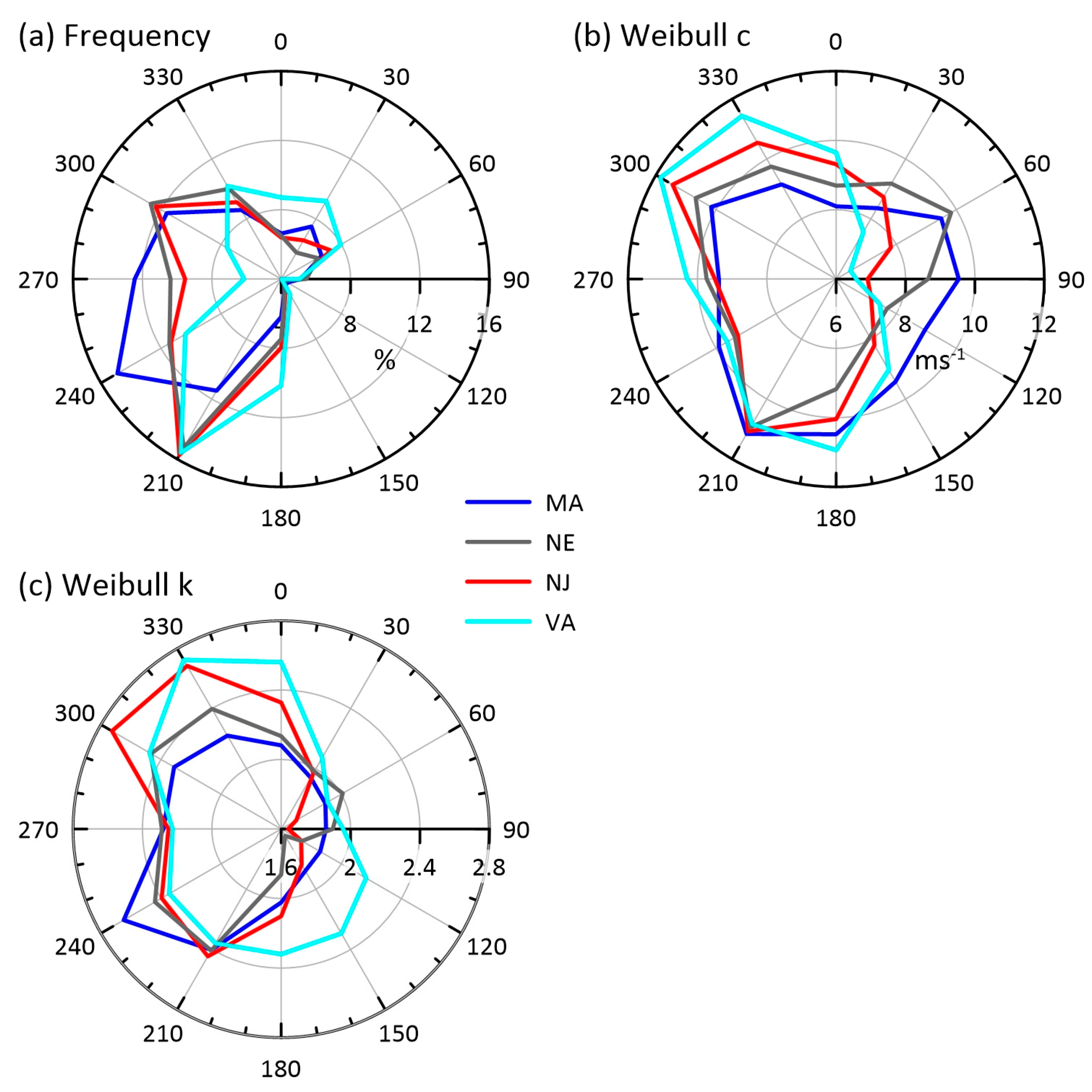
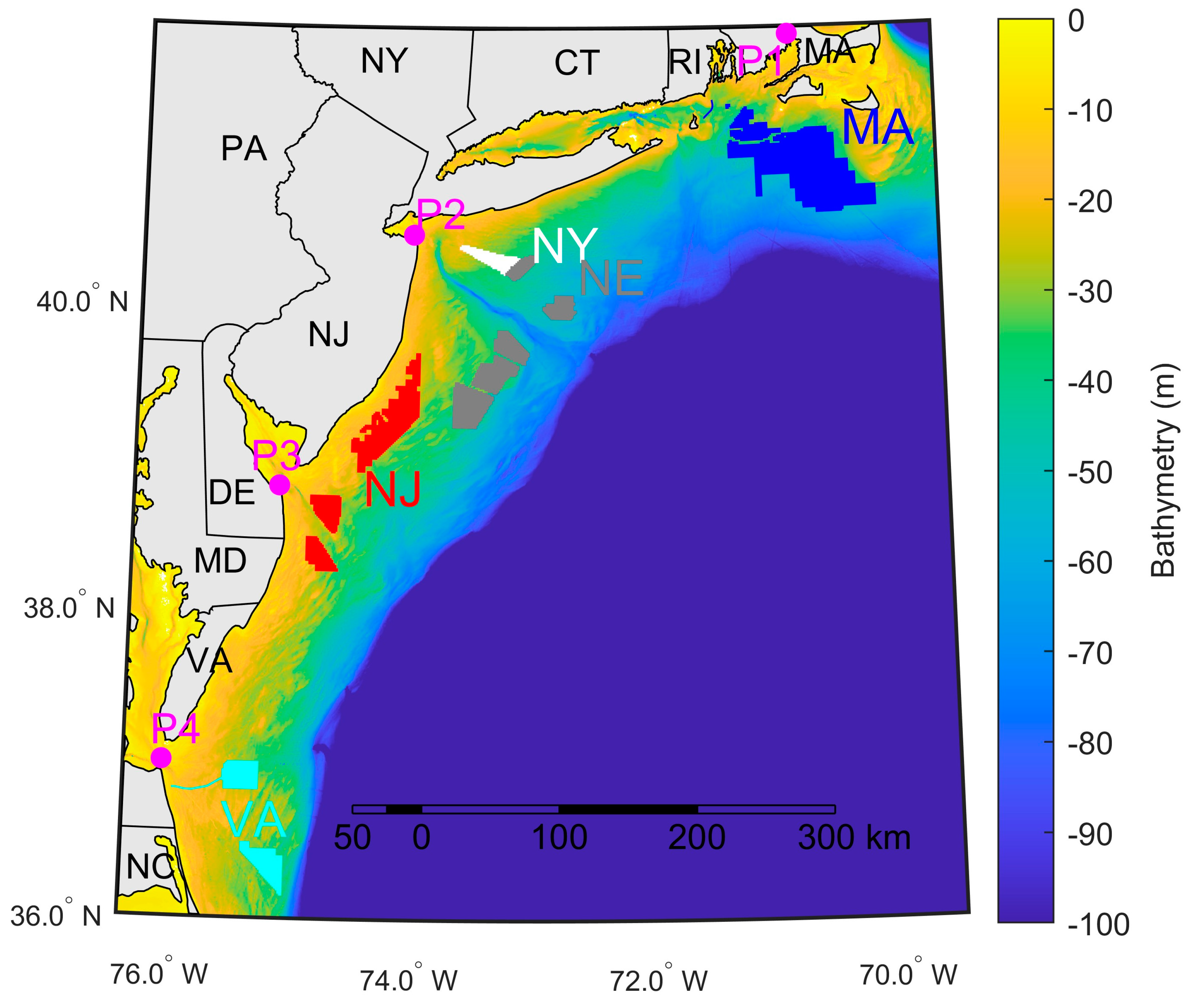
To generate the freestream wind climate, 40 years of hourly u (west–east) and v (south–north) wind components at 100 m height from ERA5 reanalysis [10] in the center of each LA group were used to compute the wind direction frequency and Weibull scale and shape distribution parameters (c and k) [49,50] of the wind speed probability distribution in 30° sectors using maximum likelihood estimation:

$$\mathrm{f}\left(\mathrm{U}\right)=\frac{\mathrm{k}}{\mathrm{c}}{\left(\frac{\mathrm{U}}{\mathrm{k}}\right)}^{\mathrm{k}-1}\mathrm{e}\mathrm{x}\mathrm{p}\left[-{\left(\frac{\mathrm{U}}{\mathrm{c}}\right)}^{\mathrm{k}}\right]$$

(7)

This wind climate (Figure 2) was used for both microscale wake models. However, it must be acknowledged that the assumption of an average wind speed and direction distribution may not reflect the variability of offshore wind conditions. In the ERA5 data, all LA groups were dominated by flow from the southwest sector, but the highest wind speeds (and, hence, Weibull scale factor) in LA groups NE, NJ and VA were associated with northwesterly flow due, in part, to longer over water fetch for northwesterly than southwesterly flow (Figure 1).

(ii)

In the NOJ model, k was set to 0.04 (Equations (4) and (5)).

(iii)

For the Fuga wake model, default parameters were used. Offshore roughness length (z₀) was set to 0.0001 m, the atmospheric boundary layer was assumed to be near-neutral and the PBLH = 400 m.

(iv)

The wind turbine power (P) and thrust (C_t) coefficients that describe the power production and thrust on the flow as a function of inflow wind speed derive from the 15 MW IEA reference wind turbine [24]. Thus, annual energy production (AEP) is the total power from wind turbines in each LA group computed as the sum of power from all wind turbines derived using the Weibull distributed wind speeds in each wind direction sector.

Figure 2. Wind climate computed using output from the ERA5 reanalysis at the center of each LA group (shown by the colored lines; MA, NE, NJ and VA) for a height of 100 m above sea level. (a) Frequency of flow in each 30° directional sector. (b) Weibull c (scale) parameter in each 30° directional sector. (c) Weibull k (shape) parameter in each 30° directional sector.

Figure 2. Wind climate computed using output from the ERA5 reanalysis at the center of each LA group (shown by the colored lines; MA, NE, NJ and VA) for a height of 100 m above sea level. (a) Frequency of flow in each 30° directional sector. (b) Weibull c (scale) parameter in each 30° directional sector. (c) Weibull k (shape) parameter in each 30° directional sector.

Simulations for these wind climates and the IEA 15 MW reference wind turbine were performed with both NOJ and Fuga for a range of wind turbine layouts that are described in the next section.

2.2. Lease Areas and Wind Turbine Layouts

Seven different wind turbine layouts were investigated herein and applied to the LA groups (Figure 3). These layouts were designed to sample across the range of installed capacity density (ICD) for European offshore windfarms. The majority of those windfarms had an ICD of 3–8 MW/km², although two were reported as having ICD above 12 MW/km² [25]. The wind turbine layouts considered (Table 2) were:

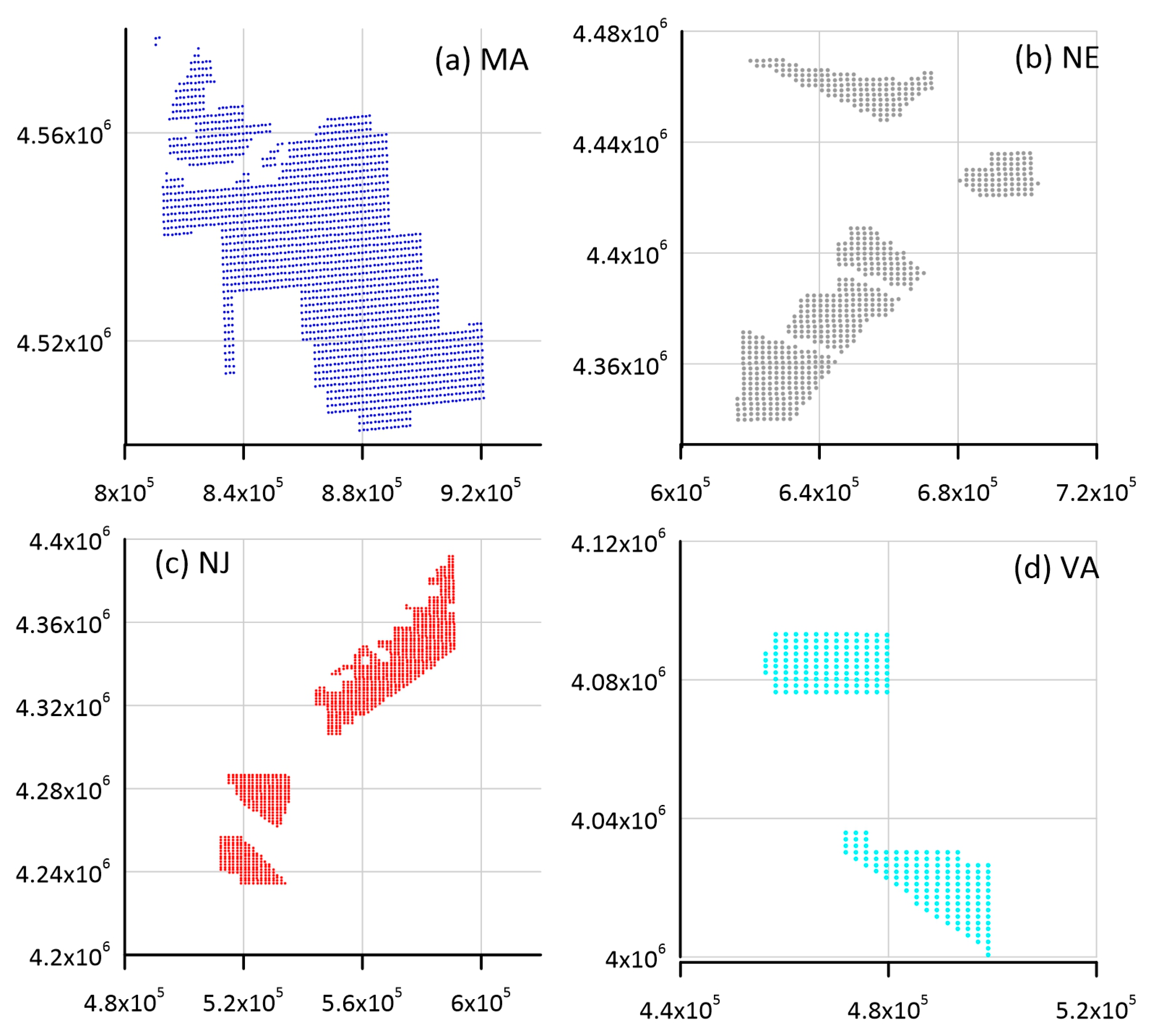
• CNTR: In this layout, wind turbines were deployed on an equally spaced north–south and east–west grid with a spacing of 1.85 km. For the 15 MW IEA reference wind turbines, this equated to a spacing of 7.7 D and an ICD of approximately 4.3 MW/km². The LA groups; MA, NE, NJ and VA had 1071, 666, 624 and 255 wind turbines, respectively, for this layout (Figure 3).
• CORR: In this layout, every sixth north–south column of wind turbines was removed to generate a marine corridor. This led to an average ICD of approximately 3.5 MW/km². Implementation of these corridors may enable multiple use of these areas [51] (e.g., enable fishing), address shipping safety concerns [52] and mitigate wildlife impacts [53].
• HALF: In this layout, wind turbines were deployed with increased spacing in the west–east and north–south directions to reduce to half the number of turbines relative to CNTR. The resulting ICD was approximately 2.1 MW/km².
• DOUBLE: In this layout, wind turbines were deployed with decreased spacing in the west–east and north–south directions to double the number of turbines relative to CNTR. The resulting ICD was approximately 8.6 MW/km².
• RO30: In this layout, wind turbines were deployed on an equally spaced north–south and east–west grid with a turbine spacing of 1.85 km (as in CNTR), the locations were then rotated by +30° (i.e., in a clockwise direction) around a center axis in order to increase the wind turbine separation along the south-southwest to north-northeast prevailing wind direction (Figure 2).
• RO60: In this layout, wind turbines were deployed on an equally spaced north–south and east–west grid with a turbine spacing of 1.85 km (as in CNTR), the locations were then rotated by +60° (i.e., in a clockwise direction) around a center axis in order to increase the wind turbine separation along the west-southwest to east-northeast prevailing wind direction (Figure 2).
• 6MWD: In this layout, wind turbines were deployed on an equally spaced north–south and east–west grid with an approximate separation of 1.6 km for an ICD of approximately 6 MW/km².

Figure 3. Offshore wind energy lease area groups; (a) MA (blue), (b) NE (grey), (c) NJ (red) and (d) VA (cyan) in UTM coordinates with the wind turbine locations for the CNTR layout—West–East and North–South grid with 1.85 km spacing. Each grid box shown (grey lines) is 40 km by 40 km.

Figure 3. Offshore wind energy lease area groups; (a) MA (blue), (b) NE (grey), (c) NJ (red) and (d) VA (cyan) in UTM coordinates with the wind turbine locations for the CNTR layout—West–East and North–South grid with 1.85 km spacing. Each grid box shown (grey lines) is 40 km by 40 km.

Table 2. Number of wind turbines in each LA group for each of the layouts.

Lease Area Group (Area km2)	CNTR	CORR	HALF	DOUB	RO30	RO60	6MWD
MA (3675)	1071	898	532	2162	1082	1090	1475
NE (2188)	666	558	334	1342	671	657	889
NJ (2105)	624	521	318	1193	595	603	801
VA (952)	255	226	124	533	268	266	338

Table 2. Number of wind turbines in each LA group for each of the layouts.

Lease Area Group (Area km2)	CNTR	CORR	HALF	DOUB	RO30	RO60	6MWD
MA (3675)	1071	898	532	2162	1082	1090	1475
NE (2188)	666	558	334	1342	671	657	889
NJ (2105)	624	521	318	1193	595	603	801
VA (952)	255	226	124	533	268	266	338

Three of these layouts, CNTR, CORR and HALF, replicated those used in our earlier WRF simulations [16].

In each layout, the wind turbine locations were georeferenced within each of the irregular polygons that describe the LA as follows. The exact position of each wind turbine was determined by assigning the first wind turbine to the northeast corner of the LA. Wind turbines were then spaced at the prescribed distance moving south in the LA until the southern boundary was reached. The next wind turbine was placed at the prescribed spacing west of the first turbine and the next column of turbines was located moving southwards and so on. For the rotated layouts, a larger area is first filled with wind turbines with the selected spacing and it is then rotated at the given angle retaining only those turbines still within the LA but ensuring the LA is full and does not have any gaps. Note, there are small variations in the actual ICD in the LA groups that are introduced by the irregularity of LA polygons.

2.3. Levelized Cost of Energy (LCoE)

There are relatively few published studies of offshore wind farm costs and their breakdown. Thus, in the following, in addition to highlighting the assumptions employed herein, a brief survey of past work is presented.

CAPEX costs (expressed here in USD million/MW) are dictated by a range of factors including: wind turbine purchase price, project management costs and a range of components that are often grouped in balance of system (BOS) costs. BOS include factors such as: (a) foundation costs that are determined in part by water depth, (b) distance to port that dictates costs associated with transport during installation and also impacts OPEX costs, (c) length and capacity of internal electrical cabling, which is determined, in part, by the wind turbine spacing, (d) length and capacity of external cabling that is largely determined by the distance to the onshore substation. For fixed bottom offshore wind turbines, according to the NREL model, the total CAPEX was $3.77 million/MW, with about half from BOS costs (

Table 3. CAPEX estimates in US $ million per MW of installed capacity from previous work along with the breakdown by the sectors that contribute to CAPEX. Where contributions to BOS are available they are shown in italics (i.e., the values sum to BOS).

	Liang [57]	%	NREL 3 [54,55,58,59]	%	BVG 2 [56]	%	IEA [60]		BOSi 4 Equation (8)	%
CAPEX/MW ($ million)	3.05		3.77		3.38		3.54		3.84
Project management 1	0.45	14.80	0.67	17.8	0.58	17.11	0.52	14.69	0.67	17.45
Turbine	1.2	39.30	1.3	34.6	1.44	42.77	1.5	42.37	1.37	35.68
BOS	1.4	45.90	1.8	47.5	1.36	40.12	1.52	42.94	1.80	46.88
Foundation	0.8	26.23			0.52	15.48	0.7	19.77	1.02	26.56
Internal cable	0.01	0.33			0.06	1.73	0.13	3.67	0.08	2.08
Export cable	0.08	2.62			0.49	14.36	0.37	10.45	0.04	1.04
Sub-station offshore	0.34	11.15			0.21	6.22	0.2	5.65	0.44	11.46
Sub-station onshore	0.17	5.57			0.08	2.368	0.14	3.95	0.22	5.73

¹ Development, project management and decommissioning if specified [56]. ² Converted from £ using 1.376 for 2021 [56]. ³ NREL BOS costs assigned between foundation and electrical infrastructure for a wind farm of ~200 MW with a 3 MW turbine in water depth of 28 m, 40 km from shore [54]. ⁴ The initial costs BOS_i are estimated for 40 km distance from shore and 160 km of internal cable.

) [36]. The breakdown of BOS costs was as follows: 3% development, 4% engineering and management, 1% port and staging, 28% substructure/foundation, 31% electrical infrastructure, 32% assembly and infrastructure and 2% plant commissioning [54,55]. An analysis by BVG associates for a ‘typical’ UK offshore wind farm found a total CAPEX of $3.38 million/MW, excluding decommissioning costs estimated as $0.42 million/MW [56]. This is for an average lifetime of 27 years with a weighted average cost of capital of 6%. The low BOS estimates relative to the NREL BOS model (Table 3) may be a reflection of moderate water depths for most UK offshore wind farms compared with those expected in the US [6].

The initial lease areas along the US East Coast that were considered here have water depth of less than about 100 m and hence are suitable for installation of bottom-mounted turbines [61]. Based on Table 3, our first estimate of BOS_i for the US East Coast is assumed as $1.8 million/MW based on the following components:

$${\mathrm{B}\mathrm{O}\mathrm{S}}_{\mathrm{i}}=\mathrm{F}+\mathrm{S}\mathrm{S}+\mathrm{E}\mathrm{C}+\mathrm{I}\mathrm{T}\mathrm{C}$$

(8)

where:

F is the foundation cost

SS is the substation total cost (onshore and offshore)

EC is the external or export cable cost;

ITC is the internal cable cost.

Assuming from the NREL studies [55,58,59] that the total BOS_i is $1.8 million, the costs fixed by MW (foundation and sub-stations) are allocated based on the cost breakdown from [57] that have to be adjusted slightly to allow for greater contribution from internal cables (described below). Thus, F was 26.5% of the total cost, and F = $1.02 million/MW. Similarly for the offshore and onshore substations, values of $0.22 million/MW and $0.44 million/MW were obtained from the percentage contribution to BOS_i.

The length of the external cable was computed as the mean distance to shore from the LA groups. It was assumed the external cable cost was USD1.42 million per km based on estimates from Europe [62]. The exchange rate was assumed to be the average of rates during 2021: $1 = EUR 1.183 (https://www.exchangerates.org.uk, accessed on 16 April 2023).

The internal cable costs (including installation) were modeled at 0.465, 0.544 and USD 0.632 million per km [57], and we selected $0.544 million/km for use herein. An analysis of the sensitivity of the results to this range is given in Section 3.1. An estimate of the total length of internal cables for each layout and each lease area (ITD) was computed as follows. We first computed the minimum total internal cable distance as the sum of the minimum distances between turbines (ITD_min = the number of wind turbines in a given layout multiplied by the spacing (minimum distance)). An estimate of the maximum internal cable (ITD_max) length was generated by summing the minimum distances between all the adjacently numbered wind turbines in the array. Since these were numbered here top right to bottom left, every new column (a row is an east–west line of wind turbines and a column is a north–south line of wind turbines) required an addition of cable equal to the length of the north–south column which considerably extended the internal cable total. The average of these two estimates was assumed to represent the likely span of internal cable lengths for a given contiguous lease area:

$$\mathrm{I}\mathrm{T}\mathrm{D}=({\mathrm{I}\mathrm{T}\mathrm{D}}_{\mathrm{m}\mathrm{i}\mathrm{n}}+{\mathrm{I}\mathrm{T}\mathrm{D}}_{\mathrm{m}\mathrm{a}\mathrm{x}})/2$$

(9)

If the LA group comprises several adjacent areas, the maximum includes the row/column distances between the continuous areas plus twice the distance between adjacent areas, which supposes these would be linked by a cable. Because the adjacent areas were typically within ~30 km, this did not greatly impact the maximum cable length. This average was used in the current model rather than a more computationally expensive cable optimization algorithm.

Some economies of scale were likely to be realized for very large wind farms. These reduced costs per installed MW will derive from, e.g., lower costs per MW for export cabling and offshore substations [59]. Past work suggested increasing installed capacity (IC) from 250 MW to 2.5 GW decreases BOS by 15.6%, although most of the reduction occurred as the wind farm size increased to 1 GW [59]. Herein, if IC in a given lease area exceeded 1 GW, a 15% reduction was applied to decrease BOS:

$${\mathrm{B}\mathrm{O}\mathrm{S}}_{\mathrm{j}}={\mathrm{B}\mathrm{O}\mathrm{S}}_{\mathrm{j}}\times (1-0.0015\times \mathrm{I}\mathrm{C})$$

(10)

Linear interpolation was used between a scaling factor of 0 and 0.0015 for wind farms with IC > 250 MW and < 1 GW. Using Equation (10), a new estimate of BOS (BOS_j) was derived from the initial estimate BOS_i for each LA group.

The values given above of the balance of systems are for a reference distance to shore of 40 km. However, most of the components of BOS and installation were very sensitive to distance to shore (X_s). Indeed, only the onshore substation and internal cabling are independent of X_s [56]. Past research suggested BOS scales with X_s for values of 5 to 100 km [54]. For simplicity, in this study, the following relationship was fitted to output from that more complex model [54] to give the final estimate of the balance of systems (see Figure 4):

$$\mathrm{B}\mathrm{O}\mathrm{S}=0.23\times {\mathrm{B}\mathrm{O}\mathrm{S}}_{\mathrm{j}}\times {\mathrm{X}}_{\mathrm{s}}^{0.4}$$

(11)

In determining total CAPEX, D_p is project management and is set as D_p = USD $0.67 million/MW based on the NREL 2022 Annual Technology Baseline [37]. T is wind turbine purchase price and is set as USD $1.3 million/MW based on the NREL 2022 Annual Technology Baseline [36].

Equations (8)–(11) provided a simplified BOS cost model that can account for distance to the coast X_s (as a proxy for water depth) together with some modification for economies of scale for larger wind farms and for internal cable length dependent on turbine layout. The BOS approximation (Equation (11) and Figure 4) showed good agreement with results of the more complex NREL balance of system model [54] in terms of the variation of BOS with X_s up to 120 km (Figure 4). Likely additional parameters such as water depth and significant wave height were also needed to modify foundation costs and access windows [63]. Figure 4 shows CAPEX and BOS and their relationship with distance from the coast where CAPEX was set to 100% at 40 km from the coast and CAPEX at 20 km to the coast was ~90% of those at 40 km. As distance increased to over 120 km from the coast, CAPEX increased to nearly 140% of those at 40 km.

In the calculation of LCoE from each of the LA groups, the average distance to the coast (X_s, the scaling factor in Equation (11)) was based on selection of one plausible port location for each LA group. These are shown in Figure 1 in magenta, where P1 is for MA, P2 for NE, P3 for NJ and P4 for VA. The minimum distance to the port location from each wind turbine in a LA group was used to compute average X_s for each LA group of: 113 km for NE, 100 km for MA, 99 km for NJ and 55 km for VA. For context, European offshore wind farms installed in 2020 had an average X_s of 52 km, and the mean water depth was 44 m [3].

The final estimate of CAPEX per installed MW based on the assumptions used herein is given in Figure 5 for a X_s of 40 km and a total installed capacity of <250 MW, along with estimates from four other studies. The primary differences between these cost models were in the techniques used to estimate BOS, as project costs and turbine costs were relatively fixed. As indicated in Figure 5, the largest variation was in the foundation costs and the electrical infrastructure, which was expected, since these are dependent not just on the distance to the nearest port/point of connection but also the wind farm size and the water depth. Nonetheless, the overall costs were relatively similar at between $3 and 3.8 million per installed MW.

3. Results

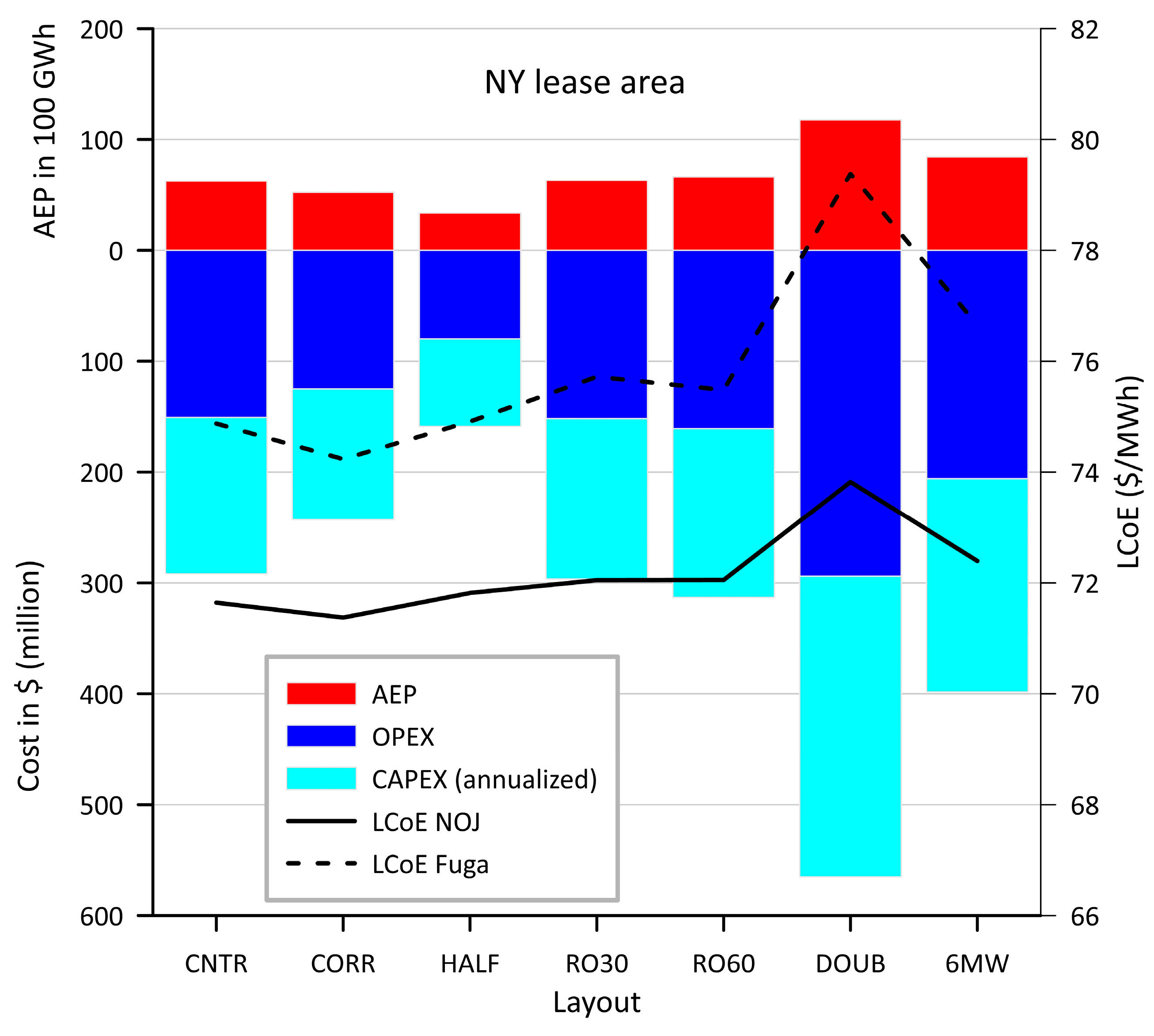
3.1. Illustrative Example of Research Methodology and Results: NY Lease Area

To provide an example of how the microscale simulations are run and how the different wake formulations and estimated AEP influence LCoE, details are given in this section for the original NY lease area (see Figure 1 and Table 1, OCS-A 0512). This lease area had a relatively small area of 321 km² and in the CNTR layout, comprised 89 wind turbines for an IC of 1.335 GW. It was, thus, representative of some operating offshore wind farms that exhibited CF of 38% to 42% [29,30,31]. To aid interpretability, in these simulations, no other lease areas were populated with wind turbines; thus, no array-to-array wake interactions were considered.

Using forty years of ERA5 reanalysis data from 1979–2018, the mean wind speed at 100 m at the NY lease area centroid was 8.55 ms⁻¹, and the Weibull shape and scale parameters were 9.65 ms⁻¹ and 2.13, respectively [7]. Analyses of output from the ERA5 reanalysis using the Gumbel distribution yielded a 50-year return period wind speed of 34.5 ms⁻¹, and a 50-year return period significant wave height of 5.6 m [7]

Once the wind climate was described in terms of the Weibull distribution parameters in 30° directional sectors and the frequency of occurrence of flow each sector, and the wind turbine locations were calculated for each layout, the PyWake platform was used to calculate the AEP using the NOJ and Fuga wake parameterizations. The excellent wind resource yielded high AEP and CF for all layouts and both wake models (

Table 4. Analyses of AEP and CF from the NY lease area (OCS-A 0512) for the different layouts from the NOJ and Fuga wake models calculated using the 40-year wind climate calculated using hourly output from ERA5. #WT = number of wind turbines.

Wake Model →				NOJ				Fuga
Layout	#WT	ICD (MW/km2)	Min. Distance between WT (km)	AEP (GWh/y)	AEP (GWh/y) per WT	AEP (GWh/y) per km2	CF (%)	AEP (GWh/y)	AEP (GWh/y) per WT	AEP (GWh/y) per km2	CF (%)
CNTR	89	4.2	1.85	6242	70	19	53.4	6105	69	19	52.2
CORR	74	3.5	1.85	5216	70	16	53.6	5126	69	16	52.7
HALF	47	2.2	2.62	3357	71	10	54.4	3326	71	10	53.9
DOUB	174	8.1	1.31	11775	68	37	51.5	11173	64	35	48.9
RO30	90	4.2	1.85	6298	70	20	53.3	6154	68	19	52.0
RO60	95	4.4	1.85	6649	70	21	53.3	6499	68	20	52.1
6MWD	122	5.7	1.57	8446	69	26	52.7	8162	67	25	50.9

). However, even for this relatively small wind farm, there were notable differences in CF from the two wake models, with Fuga consistently generating lower AEP due to the larger wake losses. The double density layout (DOUB) had the lowest CF, consistent with the larger wake losses, but remained above 48% for both wake models. Little or no benefit was seen from use of the rotated layouts in terms of CF, which had increased WT separation along a southwest to northeast axis, despite the high prevalence of southwesterly winds (Figure 2 and Table 4).

For this lease area, the distance to port (P) was 36 km (Figure 6). This distance (X_s) was used to compute the cost of the external cable and also to scale BOS (Equation (11)). As shown in Figure 6, the water depths in this LA ranged between 25 and 40 m and generally follow a west–east gradient (i.e., exhibit a dependence on X_s) consistent with the scaling of foundation and other BOS costs with distance to the port (P). For the CNTR layout shown in Figure 6, the estimated ITD (Equation (9)) was 206.5 km. For the three different cable costs; USD million/km of 0.465, 0.55 and 0.632 [57], this resulted in total costs in the range of USD96–130.5 million. For comparison, at the Horns Rev 1 offshore wind farm, which had 80 wind turbines with rotor diameter of 80 m and 7D equidistant spacing (i.e., 0.56 km) [66], a cabling study of regular versus irregular layouts was undertaken [67]. The baseline cable length spacing was 65 km, while the improved (irregular) layout had 58 km of internal cable, resulting in a reduction of 3.3% in LCoE. Based on the ITD model used here (Equation (9)), for the Horns Rev case, the minimum cable would be 44 km and the maximum ~66 km, giving an average of 55 km. So, our approximation seems appropriate and, potentially, could be further simplified to a ratio of 1.25 times the minimum distance multiplied by the inter-turbine distance (for regular grids). Note the irregular shape of the NY LA (Figure 6) increased the cable length using this simplified approach compared to a rectangular grid, as in the Hons Rev case. ITD costs for the HALF layout for NY were approximately double from the minimum cost in the HALF layout to triple in the maximum cost in the DOUB layout (

Table 5. Internal cable lengths (ITD) and costs (for three different cost assumptions [57]) for the NY lease area; OCS-A 0512, along with total CAPEX and total OPEX based on the 0.544 million/km cable cost for three different wind turbine layouts; CNTR, DOUB and HALF.

Layout	Minimum Turbine Spacing (D)	Internal Cable Length (ITD) (km)	Internal Cable Cost (Million $ per km Top Row, Remaining Rows Total Cost Million $)			Total CAPEX (Million $)	Total OPEX (Million $/yr)
			0.465	0.544	0.632
CNTR	7.7	163	76	89	103	4487	151
DOUB	5.5	230	107	125	145	8695	296
HALF	10.9	123	57	67	78	2444	80

). The contribution from ITD ranged from 1.9 to 3.1% of CAPEX and, therefore, the variability in ITD with wind turbine spacing cannot be disregarded, and it was included in the LCoE.

Final CAPEX and OPEX for the NY lease area (OCS-A 0512) broadly scaled with the number of turbines (Table 5 and Figure 7), while AEP was non-linearly dependent on the number of wind turbines due to the non-linearity in wake losses and was a function of the wake parameterization. Recall, for the CNTR layout with 89 turbines at 1.85 km spacing, the estimated AEP was 6241.7 GWh/y from NOJ and 6104.6 GWh/y based on the Fuga wake farm parameterization. The LCoE for the different layouts based on AEP from the NOJ model ranged from a low of $71.4/MWh for the CORR layout to slightly over $73.8/MWh in the DOUB layout (Figure 7). Higher wake losses using Fuga compared to NOJ give higher LCoE, e.g., from CNTR with Fuga LCoE was USD 73.3/MWh. The biggest difference in LCoE from the two wake parameterizations (Figure 7) was in the highest density layout (DOUB) with Fuga LCoE increasing to USD 77.8/MWh, which was solely a function of increased wake losses.

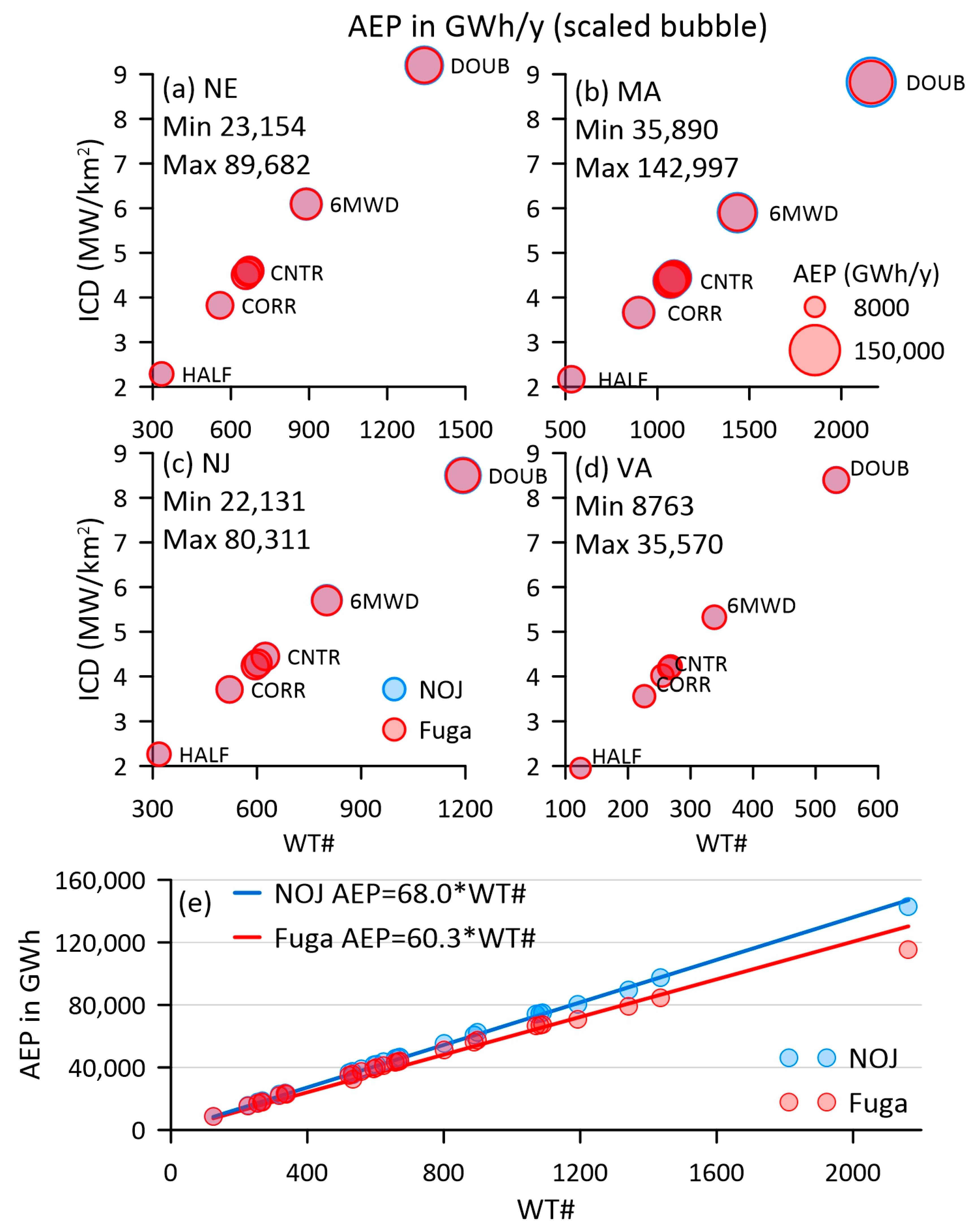
3.2. Wind Farm Modeling of Wakes and AEP for the LA Groups

For each LA group, the PyWake platform with NOJ and Fuga wake models enabled was applied to each of the seven wind farm layouts shown in Table 2 to compute AEP for the wind climate generated from ERA5. Consistent with results from the WRF simulations with the Fitch wind farm parameterization [16]; these simulations indicated that despite the very large numbers of wind turbines that were projected to be deployed over semi-continuous or continuous areas, the excellent wind resource led to high projected CF for all wind turbine layouts and all LA groups (

Table 6. Annual Energy Production (AEP) and Capacity Factors (CF) for the control layout (CNTR) for the four LA groups based on simulations with the NOJ and Fuga wake models. #WT is the number of wind turbines.

Lease Area Group	Wake Parameterization	Area (km2)	WT	AEP (GWh/y)	CF (%)
NE	NOJ	2188	666	46,317	52.9
NE	Fuga	2188	666	43,738	50.0
MA	NOJ	3675	1071	73,975	52.6
MA	Fuga	3675	1071	66,753	47.4
NJ	NOJ	2105	624	43,635	53.2
NJ	Fuga	2105	624	41,191	50.2
VA	NOJ	952	255	17,763	52.7
VA	Fuga	952	255	9024	50.5

and Figure 8). Full results are given in Appendix A. For the CNTR layout, simulated CF for all of the LA groups were 50% or above with either wind farm parameterization, with only one exception of the Fuga simulations of the MA group. The total AEP from the four LA groups for the CNTR layout of 160 to 182 TWh/yr (the range was from the two wake models) equated to approximately 4 to 4.6% of current total US electricity consumption (approx. 3930 TWh in 2021, according to data from the U.S. Energy Administration; https://www.eia.gov/energyexplained/electricity/use-of-electricity.php, accessed on 28 November 2022), which re-emphasized the importance of these LA to green transformation of the national energy supply.

Wake losses were always larger in simulations using Fuga compared to NOJ, leading to lower CF by an average of 3.5 percentage points. For the CNTR layout, the MA LA group comprised 1071, 15 MW wind turbines distributed over an area of 3675 km² for an average ICD of ~4.2 MW/km². The resulting simulated CF was five percentage points higher in simulations with NOJ. The CF was 52.6% from NOJ and 47.4% from Fuga. This difference demonstrated the much more intense deep array effect in simulations with the Fuga model that had a more robust treatment of wake generation, merging and dissipation. As discussed in detail below, the difference in AEP; 73,975 versus 66,753 GWh/yr. from NOJ and Fuga led to a substantial (USD 10/MWh) difference in LCoE for the CNTR layout and the MA LA group. The differences in AEP and CF from the two wake models were more modest for the NE, NJ and VA LA groups (Table 6). This was partly because these other LA groups were not comprised of adjoining individual lease areas and, thus, there was open water between these lease areas (see Figure 3). This allowed for partial recovery of the whole wind farm wake from each lease area within the LA group. Nevertheless, each of these LA frequently experienced lower freestream wind speeds than would be the case in the event that the upwind lease areas were not populated with wind turbines [16].

Highest CF were uniformly associated with lowest ICD and greatest wind turbine spacing (Figure 8). For the NJ and MA LA groups, the rotation of the layout to increase the wind turbine spacing along the southwest-northeast axis and, hence, prevailing wind direction did not appreciably increase AEP and CF (Figure 8). This was likely because of the size of the arrays resulting in the majority of the wind turbines being in a fully waked position for most wind directions combined with the broad distribution of wind directions (Figure 2 and Figure 3). In other words, the wake losses were mainly determined by laterally merged wakes, where the limiting factor in wake recovery was the transfer of momentum from aloft with relatively few occurrences of flow exactly down the row, where the velocity deficit was most pronounced and the wake loss effects were most pronounced [14]. For the NJ LA group, rotation of the layout actually slightly decreased AEP and CF, while for the VA LA group, there was a small positive impact from the layout rotation. This was likely because the VA LA group exhibited the most unidirectional flow along an axis oriented from 210 to 30° (Figure 2).

For smaller wind farms, there was an almost linear fit between the number of wind turbines (WT) and AEP for a regression equation with forced zero intercept (Figure 8e). However, as wind turbine numbers increased, the linear fit overpredicted AEP as wake losses increased, i.e., due to the deep array effect discussed in Section 1.2. The coefficient b in the linear fit equation:

$$\mathrm{A}\mathrm{E}\mathrm{P}=\mathrm{b}\ast \mathrm{W}\mathrm{T}\#$$

(12)

ranges b = 68.0 from NOJ simulations to b = 60.3 from Fuga. Hence, the implied increase in AEP for each additional wind turbine deployed was over 10% lower in simulations with the Fuga model. This illustrates the considerable uncertainty in wake simulations arising solely from the different parameterizations and suggests that further evaluation of the wake model parameterizations should be conducted using actual power production data from large operating offshore wind farms.

To provide context for these results, Figure 9 summarizes modeled mean CF generated for the seven layouts herein (as weighted averages from the four LA groups, where the weighting is a function of the number of wind turbines in each group for a given layout). These were compared with previous research conducted using the Weather Research and Forecasting (WRF) model with the Fitch wind farm parameterization the US East Coast lease areas (excluding those auctioned in February 2022) [18], and from the Agora study in the North Sea in Europe [68]. The simulations with WRF and the Fitch wind farm parameterization that considered three of the same layouts as employed here; CNTR, HALF and CORR, and that were performed for the original lease areas (i.e., excluding those auctioned in February 2022) indicated slightly lower CF for a given ICD than were estimated here using the microscale wake modeling [16]. The simulations with WRF generated CF that were 0.9 and 2.6 percentage points lower than Fuga and NOJ for the HALF spacing, and 4.1 and 7.9 percentage points lower than those from Fuga and NOJ for the CNTR spacing (Figure 8). These differences in CF may reflect:

• Differences in the driving wind climate—here, we used 40 years of ERA5 output, while the simulations with WRF used representative flow conditions that were frequency weighted to generate a representative CF.
• The disparity in modeled CF may also reflect the fundamental differences in terms of the ability of WRF to capture variations in PBLH and the propagation of wakes from remote lease areas. The WRF simulations indicated that, under some flow conditions, the wind farm wake (defined as the area with velocity deficits due to wakes of over 5% of the freestream wind speed) extended up to 90 km from the largest wind farm clusters, and the frequency weighted net wake extent was 2.6 times the areal extent of the lease areas.
• Conversely, here, the LA groups were modeled individually with NOJ and Fuga. Furthermore, the NOJ parameterization, which used the sum of squares of the velocity deficit when wakes were merged, tended to generate wake recovery within a few kilometers of the downstream edge of a lease area. Fuga tended to generate more persistent wakes but still did not capture the full extent of the modification of the boundary-layer and the downwind propagation of whole wind farm wakes.

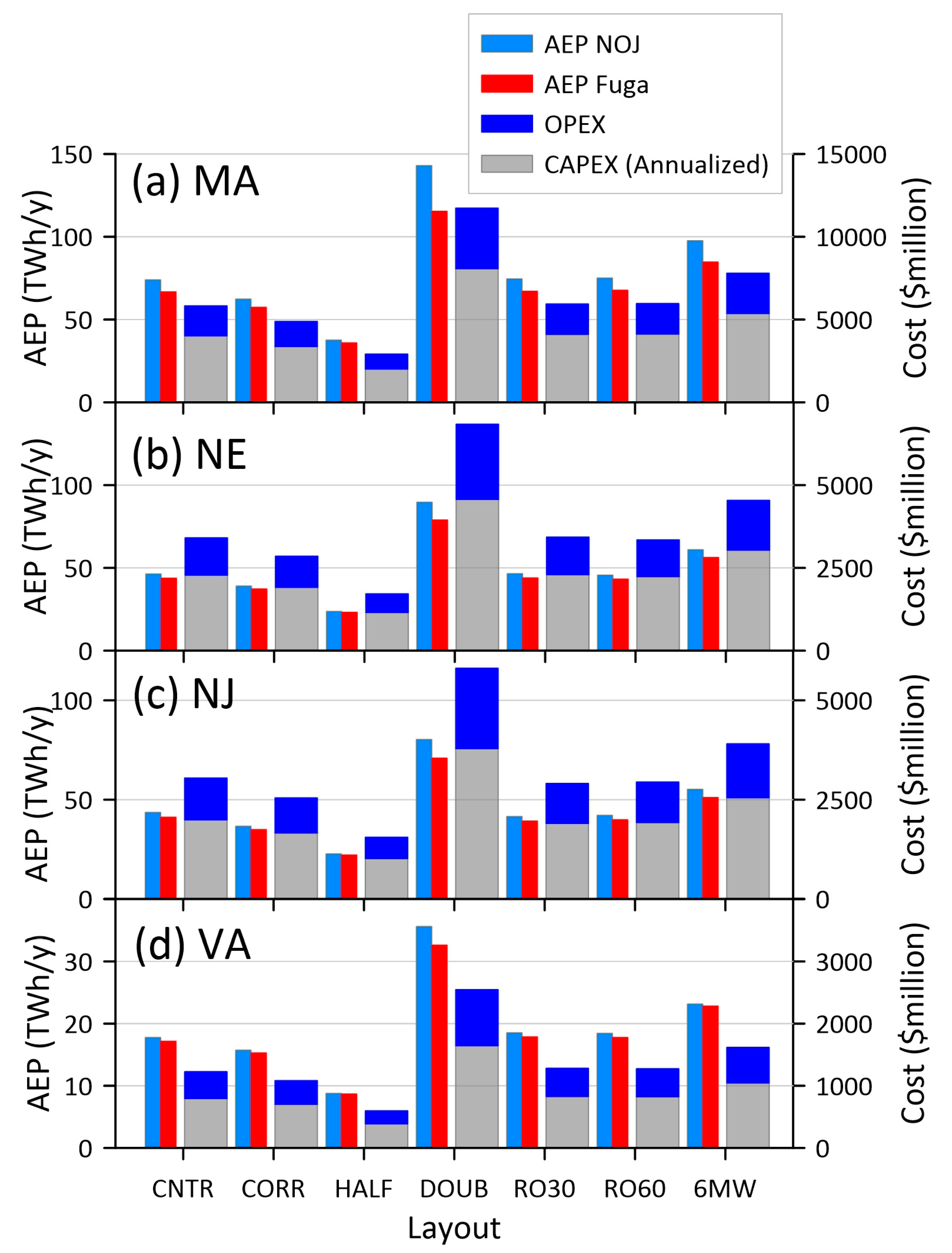
Figure 9. Relationship between modeled capacity factor (CF) and installed capacity density (ICD). (a) Mean CF from the Fuga and NOJ simulations compared with WRF results for the US East Coast and the Agora study in the North Sea Box-whisker plot at the bottom of the figure shows the 25, 50 and 75th percentile of ICD for current European offshore windfarms—two ICD above 12 MW/km² were excluded. The numbers associated with the boxplot denote the individual wind farms reported in [25]. (b) Mean CF for the seven different layouts for the individual LA groups (MA, NE, NJ and VA) as simulated using the Fuga and NOJ wake models. RO30 and RO60 have similar density to CNTR and are not labelled to improve clarity. NE and NJ typically have similar WT# and ICD. Some of the NE and NJ labels were removed to aid clarity.

Figure 9. Relationship between modeled capacity factor (CF) and installed capacity density (ICD). (a) Mean CF from the Fuga and NOJ simulations compared with WRF results for the US East Coast and the Agora study in the North Sea Box-whisker plot at the bottom of the figure shows the 25, 50 and 75th percentile of ICD for current European offshore windfarms—two ICD above 12 MW/km² were excluded. The numbers associated with the boxplot denote the individual wind farms reported in [25]. (b) Mean CF for the seven different layouts for the individual LA groups (MA, NE, NJ and VA) as simulated using the Fuga and NOJ wake models. RO30 and RO60 have similar density to CNTR and are not labelled to improve clarity. NE and NJ typically have similar WT# and ICD. Some of the NE and NJ labels were removed to aid clarity.

The differences in CF between all wind farm parameterizations and models converge as ICD was reduced, with much larger differences at the highest ICD (Figure 9). Simulations with WRF and a different wind farm parameterization for the North Sea indicated lower CF for the same ICD and wind farm extent as considered here, which was likely due to the slightly less advantageous wind resource. The critical importance of the deep array effect (i.e., large magnitude wake losses in the center of large arrays) on modeled AEP and CF is illustrated in Figure 9b (and Figure 8e) that show that, irrespective of the ICD and despite the higher wind resource, the MA LA group consistently exhibited the lowest CF in simulations with Fuga.

Figure 9a also contextualizes the ICD considered here with selected operating European offshore wind farms that had between 10 and 175 wind turbines and were built between 1995 and 2019. The ICD ranged between 3 and 18 MW/km² with averages of 5.5 MW/km² for the Baltic Sea and 6.0 MW/km² for the North Sea [25]. These wind farms were, thus, considerably smaller than those being planned along the US East Coast but, nevertheless, provided support for the range of ICD considered in this analysis.

3.3. LCoE Modeling

Current generation LCoE models used for offshore wind farm costing [54,55] typically treat CAPEX and OPEX costs per MW of installed capacity, and so, the overall project costs tend to scale linearly with the number of wind turbines. In reality, some economies of scale are to be expected in terms of efficiencies in renting or purchasing transport for installation for maintenance or in delivery costs for wind turbines. A moderate scale factor was used here (Equation (10)) but total project costs for a given LA were still dominated by the number of wind turbines in each wind turbine layout (Figure 10). Some subtler differences were evident when comparing LA groups. For example, the external cable costs were higher per MW for NE than VA because the LA group was closer to the coast, leading to lower BOS and CAPEX costs.

The relationship between the total number of turbines and the project CAPEX and OPEX scaled more linearly and with a higher multiplier with the number of wind turbines than AEP. Accordingly, even neglecting important differences from the two wake models, LCoE exhibited marked variability across the different LA groups, and differences between LCoE for different layouts were not entirely consistent across the LA groups (Figure 11). LCoE for the MA LA group, particularly using the Fuga parameterization, was substantially higher for the largest ICD considered herein (DOUB, approximately 8.6 MW/km²) (Figure 11). Despite having the best wind resource, LCoE figures were still higher for the MA group due to the large wake losses. LCoE for the smaller LA groups tended to cluster between USD 68 and USD 78 per MWh. For all except the MA LA group, increasing ICD from around 4 MW/km² to 6 MW/km² did not have a major impact on LCoE, indicating a balance between the increased power production from a greater number of wind turbines with power losses from wakes.

LCOE was most strongly impacted by the wind resource in the LA and wake losses. Hence, LCoE using the NOJ wake parameterization were always lower for a given LA than those from Fuga because Fuga simulated higher wake losses (Figure 11). The final LCoE for the MA lease area was reduced by the higher wind resource [7] but was the most impacted by wake losses because the number of turbines in the contiguous area varied from 532 in HALF to 2162 in DOUB (Figure 3). Hence, the MA LA was the most sensitive to the chosen topology and wake parameterization. The NJ and NE LA had excellent wind resources with LA separated by over 20 km of ocean (Figure 3), which allowed for some wind speed recovery between LA; hence, these showed similar results to each other. VA had the lowest wind speeds of the LA considered but the LA are the smallest of those simulated and hence have relatively small wake losses. Nonetheless, the LCoE for the most part were relatively similar for topologies with similar ICD (compare CNTR with RO30 and RO60), indicating the precise layout was less important than the overall number of turbines. This may arise because of the dominance of westerly winds in the East Coast (Figure 2) rather than dominance of flow from one directional sector.

A previous LCoE estimate for three 100 MW offshore sites in New York Bight derived a minimum of USD 123.4/MWh under the assumption of 8 MW wind turbines [57]. Based on analyses presented herein, that estimate appeared to be rather pessimistic, perhaps, in part, because it used wind speed data collected at 2 m on buoys to estimate wind turbine hub-height wind resources, which incurred substantial extrapolation errors. Other LCoE estimates suggested a mean US-based offshore wind energy LCoE of ~$84/MWh in 2021 that could fall to USD 60/MWh by 2030 [6] and may reach ~ USD 40/MWh by 2035 [69]. Those values are more consistent with results shown in Figure 11. Both that prior study and the detailed modeling presented herein suggested Power Purchase Agreement prices of USD 65–USD 74 per MWh for Vineyard Wind (OCS-A 0501) [70] were likely not sufficient. The work presented here indicated LCoE estimates for the MA LA group (in which OCS-A 0501 lies) ranged from USD 79 to USD 87 per MWh for the CNTR layout depending on the wake model employed. LCoE for this LA group were not below USD77/MWh for either the wake model or layout.

3.4. Modeling Uncertainties

It was acknowledged that the AEP and LCoE estimates presented herein were subject to a range of important caveats. Firstly, the microscale modeling employed a representative wind climate based on the long-term wind climate from ERA5 at the center of the LA groups and, hence, did not account for spatial variability across the LA groups and may not reflect the full variability of offshore wind conditions Additionally, the AEP estimates neglected wake interactions across the LA groups, which may be non-negligible [16]. Lastly, both wake models were evaluated using data from offshore wind farms that were considerably smaller than those being developed along the US East Coast. The microscale modeling presented herein gives higher capacity factors by 1–8 percentage points than were derived in prior research using mesoscale modeling [16] and, hence, these results should be viewed with caution. The straightforward parameterization of wind turbine behavior allows feedback to the physics of the atmospheric boundary-layer modification that can propagate for many tens of kilometers downstream of wind farms [16]. Nonetheless, the microscale models can more efficiently model differences in wind farm power output that arise from different wind turbine layouts or configurations.

It is also important to note that the simulations were developed in the absence of long-term high-fidelity measurements of the hub-height wind resource and its variability. The wind direction distribution and variability could be important [71], particularly if it is unidirectional, as was implied for parts of the West Coast [72]. Spatial variability of the resource across the lease areas could make layout optimization more important. Furthermore, no large wind farms were constructed, so that wake effects can be calculated from measurements on wind turbines for comparison with the models. The differences in predicted power output between the two wake parameterizations for each LA group were generally smaller than from the different layouts but remain an important source of uncertainty. Further measurements to characterize the conditions of the LA and access to power output from wind farms, as they were built out would be beneficial to reduce these uncertainties.

Projected estimates of LCoE for US offshore wind energy projects span a wide range and depend on the availability of good quality data to derive the wind resource and assumptions about CAPEX and OPEX. They were particularly challenging to make, given that no large wind farms were constructed off the US East Coast. Hence, estimates of CAPEX and OPEX used herein were also subject to uncertainty. For example, it was assumed that the distance to the closest port can be used as a proxy for external cable costs. These costs may be substantially increased if external cables were routed differently, or more than one external cable is constructed for different wind farm developers in one LA group, to provide additional security for electricity export, or because longer routes are needed to access points of connection on the grid that have spare capacity. Uncertainties in costs can be illustrated by considering the costs associated with wind turbine installation vessels (WTIV). Specialized vessels are required to both transport and safely install wind turbines including legs that can allow the vessel to be lifted from the seafloor and securely crane the tower, blade, etc. In the US, the Jones Act will require vessels transporting turbines from US ports to US wind turbine foundations to be US built and operated under a US flag [73]. The costs cited were USD 20,000 per half hour or USD 300,000 per day for rental [74] or between USD 222 million [73] and USD 500 million [74,75] for WTIV purchase. The need for specialized port facilities to be constructed, price instability due to supply chain concerns regarding components [39] and the potential for weather delays [75] add to the uncertainty in costing US offshore wind farms.

4. Discussion and Conclusions

The main contributions of the paper were the prediction of annual energy production (AEP) linked to a simplified LCoE model for the US East Coast offshore wind energy lease areas. AEP was determined from fast microscale wind farm flow modeling, using two different wake parameterizations which enabled simulation of wakes from over 2000 wind turbines in one lease area. These AEP results were utilized within a specifically developed model for prediction of LCoE from offshore wind farms to quantify the impact of different wind farm topologies on LCoE in the different lease areas. For the investigated lease areas, the LCoE ranged from USD 68 to USD 102/MWh depending on the topology, which was cost competitive with many other generation sources. The major advantage of this work was the direct link between AEP and LCoE to rapidly assess the impact of many different wind turbine topologies.

Microscale modeling of power output for offshore wind farms along the US northeast coast lease areas presented herein indicated capacity factors of 42 to 55%, depending on the precise wind turbine layout and LA under consideration. The CNTR layout that sets out wind turbines on an east–west and north–south grid with 1.85 km spacing was agreed for the most northeasterly group of wind farms to the south of Massachusetts. Simulations with this layout using 15 MW wind turbines yielded AEP of 4 to 4.6% of national electricity consumption. LCoE was estimated for seven different layouts, including CNTR that span installed capacity density of 2.1 to 8.6 MW/km². The LCoE results ranged from 68 to USD 101/MWh. The wake model applied had a profound impact on AEP and LCoE, especially for the larger lease areas, indicating further research to reduce the uncertainty in wake parameterization is warranted. For example, AEP for the largest lease area differed by 10% depending on the wake model applied. Lowest LCoE was found for the HALF layout (ICD ~ 2.1 MW/km²), but it was only marginally lower than for the CNTR layout, and there was an almost doubling of AEP under the CNTR layout relative to HALF for all of the LA groups. Although southwesterly flow was dominant, little benefit was found in terms of AEP for rotation of the layouts to increase wind turbine spacing due to relatively high occurrence of winds from other westerly sectors.

The LCoE modeling simulated costs that were broadly in line with other estimates for the US northeast coast between 68 and USD 88/MWh for most lease areas. The largest differences in the AEP under different layouts, that propagate to a higher LCoE, were for the south of Massachusetts LA at higher installed capacity densities and using the Fuga parameterization. This was despite its outstanding wind resource. If the whole lease area is fully built, there will be ~40 wind turbines in one column in parts of the lease area, resulting in very well-developed deep array effects, especially for the highest installed capacity densities. Nonetheless, given the uncertainty in the modeling and the need to ensure optimal use of each LA, it is possible that higher ICD than currently being considered could be optimal, given that LCoE remained close to USD 100/MWh.

Offshore wind energy deployments can be optimized in terms of multiple outcomes that may not yield identical results. For example, if the goal is to maximize total power production in order to displace the maximum amount of fossil fuel generation, it is likely that a higher ICD will be selected. Achieving a goal of minimized LCoE, that is, generation of electrical power at the lowest overall cost may result in a lower ICD. For private entities, it is likely that minimized LCoE is the goal.

Figure 12 compares the projected LCoE from the US East Coast offshore wind lease areas with estimated LCoE from selected other electricity generation sources (without subsidies) [76]. According to data from Lazard [76], utility scale onshore wind and solar photovoltaics had the lowest LCoE, and the estimated LCoE from offshore wind simulations presented herein were twice as expensive as onshore wind but considerably lower than nuclear and gas peaking. Price trends for onshore wind between 2009 and 2021 indicated a decline from USD 135/MWh in 2009 to below USD 40/MWh in 2021 (Figure 12), and they were consistent with expected declines in offshore wind as the technology increased market penetration [6].

References

1. Barthelmie, R.J.; Pryor, S.C. Climate Change Mitigation Potential of Wind Energy. Climate 2021, 9, 136. [Google Scholar] [CrossRef]
2. The White House. FACT SHEET: Biden Administration Jumpstarts Offshore Wind Energy Projects to Create Jobs. 2021. Available online: https://www.whitehouse.gov/briefing-room/statements-releases/2021/03/29/fact-sheet-biden-administration-jumpstarts-offshore-wind-energy-projects-to-create-jobs/ (accessed on 26 October 2022).
3. WindEurope. Offshore Wind in Europe Key Trends and Statistics 2020. 2021. p. 38. Available online: https://windeurope.org/intelligence-platform/product/wind-energy-in-europe-in-2020-trends-and-statistics/ (accessed on 27 February 2020).
4. WindEurope. Wind Energy in Europe. 2022 Statistics and Outlook for 2023–2027. 2023. p. 58. Available online: https://windeurope.org/intelligence-platform/product/wind-energy-in-europe-2022-statistics-and-the-outlook-for-2023-2027/#overview (accessed on 24 March 2023).
5. Barthelmie, R.J.; Folkerts, L.; Ormel, F.; Sanderhoff, P.; Eecen, P.; Stobbe, O.; Nielsen, N.M. Offshore wind turbine wakes measured by SODAR. J. Atmos. Ocean. Technol. 2003, 30, 466–477. [Google Scholar] [CrossRef]
6. Musial, W.; Spitsen, P.; Duffy, P.; Beiter, P.; Marquis, M.; Hammond, R.; Shields, M. 2022 Offshore Wind Technologies Market Report DOE/GO-102022-5765; Department of Energy: Washington, DC, USA, 2022; p. 126. Available online: https://www.energy.gov/eere/wind/articles/offshore-wind-market-report-2022-edition (accessed on 4 April 2023).
7. Barthelmie, R.J.; Dantuono, K.; Renner, E.; Letson, F.; Pryor, S.C. Extreme wind and waves in U.S. east coast offshore wind energy lease areas. Energies 2021, 14, 1053. [Google Scholar] [CrossRef]
8. Volcovici, V.U.S. Offshore Wind Auction Draws Record $4.37 Billion in Bids. 2022. Available online: https://www.reuters.com/business/energy/us-offshore-wind-auction-nears-4bln-third-day-bidding-2022-02-25/ (accessed on 28 February 2022).
9. BOEM. Outer Continental Shelf Renewable Energy Leases Map Book. July 2022; p. 33. Available online: https://www.boem.gov/sites/default/files/documents/renewable-energy/Leases-Map-Book-July%202022.pdf (accessed on 23 March 2023).
10. Hersbach, H.; Bell, B.; Berrisford, P.; Hirahara, S.; Horányi, A.; Muñoz-Sabater, J.; Nicolas, J.; Peubey, C.; Radu, R.; Schepers, D.; et al. The ERA5 global reanalysis. Q. J. R. Meteorol. Soc. 2020, 146, 1999–2049. [Google Scholar] [CrossRef]
11. BOEM. Outer Continental Shelf Renewable Energy Leases Map Book. 2019; p. 19. Available online: https://www.boem.gov/sites/default/files/renewable-energy-program/Mapping-and-Data/Renewable_Energy_Leases_Map_Book_March_2019.pdf (accessed on 22 July 2020).
12. Barthelmie, R.J. The effects of atmospheric stability on coastal wind climates. Meteorol. Appl. 1998, 6, 39–47. [Google Scholar] [CrossRef]
13. Larsen, G.C.; Réthoré, P.-E. TOPFARM a tool for wind farm optimization. Energy Procedia 2013, 35, 317–324. [Google Scholar] [CrossRef] [Green Version]
14. Barthelmie, R.J.; Jensen, L.E. Evaluation of wind farm efficiency and wind turbine wakes at the Nysted offshore wind farm. Wind. Energy 2010, 13, 573–586. [Google Scholar] [CrossRef]
15. Doekemeijer, B.M.; Simley, E.; Fleming, P. Comparison of the Gaussian Wind Farm Model with Historical Data of Three Offshore Wind Farms. Energies 2022, 15, 1964. [Google Scholar] [CrossRef]
16. Pryor, S.C.; Barthelmie, R.J.; Shepherd, T.J. Wind power production from very large offshore wind farms. Joule 2021, 5, 2663–2686. [Google Scholar] [CrossRef]
17. Aird, J.A.; Barthelmie, R.J.; Shepherd, T.J.; Pryor, S.C. Occurrence of Low-Level Jets over the Eastern US Coastal Zone at Heights Relevant to Wind Energy. Energies 2022, 15, 445. [Google Scholar] [CrossRef]
18. Pryor, S.C.; Barthelmie, R.J.; Shepherd, T.J.; Hahmann, A.H.; Garcia Santiago, O.M. Wakes in and between very large offshore arrays. J. Phys. Conf. Ser. 2022, 2265, 022037. [Google Scholar] [CrossRef]
19. Nygaard, N.G.; Newcombe, A.C. Wake behind an offshore wind farm observed with dual-Doppler radars. J. Phys. Conf. Ser. 2018, 1037, 072008. [Google Scholar] [CrossRef]
20. Eriksson, O.; Nilsson, K.; Breton, S.P.; Ivanell, S. Large-eddy simulations of wind farm production and long distance wakes. J. Phys. Conf. Ser. 2015, 625, 012022. [Google Scholar] [CrossRef]
21. Barthelmie, R.J.; Pryor, S.C. Wake model evaluation using data from the Virtual Wakes Laboratory. Appl. Energy 2013, 104, 834–844. [Google Scholar] [CrossRef]
22. Barthelmie, R.J.; Hansen, K.S.; Pryor, S.C. Meteorological controls on wind turbine wakes. Proc. IEEE 2013, 101, 1010–1019. [Google Scholar] [CrossRef]
23. Barthelmie, R.J.; Frandsen, S.T.; Nielsen, N.M.; Pryor, S.C.; Rethore, P.E.; Jørgensen, H.E. Modelling and measurements of power losses and turbulence intensity in wind turbine wakes at Middelgrunden offshore wind farm. Wind. Energy 2007, 10, 217–228. [Google Scholar] [CrossRef]
24. Gaertner, E.; Rinker, J.; Sethuraman, L.; Zahle, Z.; Anderson, B.; Barter, G.; Abbas, B.; Meng, F.; Bortolotti, F.; Skrzypinski, W.; et al. Definition of the IEA 15-Megawatt Offshore Reference Wind Turbine; NREL/TP-5000-75698; National Renewable Energy Laboratory: Golden, CO, USA, 2020. Available online: https://www.nrel.gov/docs/fy20osti/75698.pdf (accessed on 11 May 2020).
25. Borrmann, R.; Rehfeldt, K.; Wallasch, A.K.; Lüers, S. Capacity Densities of European Offshore Wind Farms; SP18004A1; Deutsche Windguard GmbH: Hamburg, Germany, 2018; p. 86. Available online: https://www.msp-platform.eu/practices/capacity-densities-european-offshore-wind-farms (accessed on 20 January 2021).
26. Ahsbahs, T.; Maclaurin, G.; Draxl, C.; Jackson, C.; Monaldo, F.; Badger, M. US East Coast synthetic aperture radar wind atlas for offshore wind energy. Wind. Energy Sci. 2020, 5, 1191–1210. [Google Scholar] [CrossRef]
27. Pryor, S.C.; Shepherd, T.; Volker, P.; Hahmann, A.; Barthelmie, R.J. ‘Wind theft’ from onshore arrays: Sensitivity to wind farm parameterization and resolution. J. Appl. Meteorol. Climatol. 2020, 59, 153–174. [Google Scholar] [CrossRef]
28. Fitch, A.C. Notes on using the mesoscale wind farm parameterization of Fitch et al. (2012) in WRF. Wind Energy 2016, 19, 1757–1758. [Google Scholar] [CrossRef]
29. Wind Europe. Wind Energy in Europe in 2019: Trends and Statistics; Wind Europe: Brussels, Belgium, 2020; p. 25. Available online: https://windeurope.org/wp-content/uploads/files/about-wind/statistics/WindEurope-Annual-Statistics-2019.pdf (accessed on 6 October 2020).
30. Enevoldsen, P.; Jacobson, M.Z. Data investigation of installed and output power densities of onshore and offshore wind turbines worldwide. Energy Sustain. Dev. 2021, 60, 40–51. [Google Scholar] [CrossRef]
31. Jorgensen, B.H.; Holtinnen, H.; D’ahlgaard, K.; Rosenfeldt Jakobson, K.; Marti, I. IEA Wind TCP Annual Report 2019; International Energy Agency: Pairs, France, 2020; p. 53. ISBN 978-87-93549-78-4. Available online: http://community.ieawind.org (accessed on 11 May 2020).
32. Larsen, T.J.; Madsen, H.; Larsen, G.; Hansen, K.S. Validation of the Dynamic Wake Meander Model for Loads and Power Production in the Egmond aan Zee Wind Farm. Wind Energy 2012, 16, 605–624. [Google Scholar] [CrossRef] [Green Version]
33. Barthelmie, R.J.; Larsen, G.C.; Mølgaard Pedersen, M.; Pryor, S.C. Microscale modelling of wind turbines in the New York offshore lease area. J. Phys. Conf. Ser. 2022, 2265, 022040. [Google Scholar] [CrossRef]
34. Mahulja, S.; Larsen, G.C.; Elham, A. Engineering an optimal wind farm using surrogate models. Wind Energy 2018, 21, 1296–1308. [Google Scholar] [CrossRef]
35. Réthoré, P.-E.; Fuglsang, P.; Larsen, P.C.; Buhl, T.; Larsen, T.J.; Madsen, H.A. TOPFARM: Multi-fidelity optimization of wind farms. Wind Energy 2014, 17, 1797–1816. [Google Scholar] [CrossRef] [Green Version]
36. National Renewable Energy Laboratory. 2022 Annual Technology Baseline (ATB) Cost and Performance Data for Electricity Generation Technologies [Data Set]; National Renewable Energy Laboratory: Golden, CO, USA, 2022. Available online: https://data.openei.org/submissions/5716 (accessed on 6 April 2023).
37. Sørensen, J.N.; Larsen, G.C. A Minimalistic Prediction Model to Determine Energy Production and Costs of Offshore Wind Farms. Energies 2021, 14, 448. [Google Scholar] [CrossRef]
38. Nunemaker, J.; Matt, S.; Hammond, R.; Duffy, P. ORBIT: Offshore Renewables Balance-of-System and Installation Tool. NREL/TP-5000-77081; National Renewable Energy Laboratory: Golden, CO, USA, 2020. Available online: https://www.nrel.gov/docs/fy20osti/77081.pdf (accessed on 26 October 2022).
39. Richards, H. Energy Prices Threaten Mass. Offshore Wind Project. Energy Wire 11/01/202. 2022. Available online: https://www.eenews.net/articles/energy-prices-threaten-mass-offshore-wind-project/ (accessed on 24 March 2023).
40. Pedersen, M.M.; van der Laan, P.; Friis-Møller, M.; Rinker, J.; Réthoré, P.-E. DTUWindEnergy/PyWake: PyWake (Version v1.0.10). Zenodo. 2019. Available online: https://zenodo.org/record/2562662 (accessed on 3 August 2021).
41. Jensen, N.O. A Note on Wind Turbine Interaction; Risø-M-2411; Risø National Laboratory: Roskilde, Denmark, 1983; p. 16.
42. Barthelmie, R.J.; Folkerts, L.; Rados, K.; Larsen, G.C.; Pryor, S.C.; Frandsen, S.; Lange, B.; Schepers, G. Comparison of wake model simulations with offshore wind turbine wake profiles measured by sodar. J. Atmos. Ocean. Technol. 2006, 23, 888–901. [Google Scholar] [CrossRef]
43. Katic, I.; Højstrup, J.; Jensen, N.O. A simple model for cluster efficiency. In Proceedings of the European Wind Energy Association, Rome, Italy, 7–9 October 1986; pp. 407–409. [Google Scholar]
44. Barthelmie, R.J.; Pryor, S.C.; Frandsen, S.T.; Hansen, K.; Schepers, J.G.; Rados, K.; Schlez, W.; Neubert, A.; Jensen, L.E.; Neckelmann, S. Quantifying the impact of wind turbine wakes on power output at offshore wind farms. J. Atmos. Ocean. Technol. 2010, 27, 1302–1317. [Google Scholar] [CrossRef]
45. Cañadillas, B.; Foreman, R.; Steinfeld, G.; Robinson, N. Cumulative Interactions between the Global Blockage and Wake Effects as Observed by an Engineering Model and Large-Eddy Simulations. Energies 2023, 16, 2949. [Google Scholar] [CrossRef]
46. Ott, S.; Berg, J.; Nielsen, M. Linearised CFD Models for Wakes; Risoe-R-1772(EN); DTU: Roskilde, Denmark, 2011; Available online: https://orbit.dtu.dk/en/publications/linearised-cfd-models-for-wakes(c29803f3-a1eb-45ab-b73f-ede444928477).html: (accessed on 26 July 2019).
47. Troen, I.; Petersen, E.L. European Wind Atlas; Risø National Laboratory: Roskilde, Denmark, 1989; p. 656.
48. Ott, S.; Sogachev, A.; Mann, J.; Jørgensen, H.E.; Frandsen, S.T. Applying Flow Models of Different Complexity for Estimation of Wind Turbine Wakes. In Proceedings of the European Wind Energy Conference and Exhibition, Marseilles, France, 16–19 March 2009; p. 8. Available online: https://backend.orbit.dtu.dk/ws/portalfiles/portal/3740046/2009_17.pdf (accessed on 26 April 2022).
49. Pryor, S.C.; Nielsen, M.; Barthelmie, R.J.; Mann, J. Can satellite sampling of offshore wind speeds realistically represent wind speed distributions? Part II: Quantifying uncertainties associated with sampling strategy and distribution fitting methods. J. Appl. Meteorol. 2004, 43, 739–750. [Google Scholar] [CrossRef]
50. Wilks, D.S. Statistical Methods in the Atmospheric Sciences; Academic Press: Oxford, UK, 2011; Volume 100. [Google Scholar]
51. Gusatu, L.F.; Yamu, C.; Zuidema, C.; Faaij, A. A spatial analysis of the potentials for offshore wind farm locations in the North Sea region: Challenges and opportunities. ISPRS Int. J. Geo-Inf. 2020, 9, 96. [Google Scholar] [CrossRef] [Green Version]
52. Mehdi, R.A.; Schröder-Hinrichs, J.-U.; van Overloop, J.; Nilsson, H.; Pålsson, J. Improving the coexistence of offshore wind farms and shipping: An international comparison of navigational risk assessment processes. WMU J. Marit. Aff. 2018, 17, 397–434. [Google Scholar] [CrossRef] [Green Version]
53. Petruny, L.M.; Wright, A.J.; Smith, C.E. Getting it right for the North Atlantic right whale (Eubalaenaglacialis): A last opportunity for effective marine spatial planning? Mar. Pollut. Bull. 2014, 85, 24–32. [Google Scholar] [CrossRef] [PubMed]
54. Maness, M.; Maples, B.; Smith, A. NREL Offshore Balance-of-System Model; NREL/TP-6A20-66874. 2017; p. 56. Available online: https://www.nrel.gov/docs/fy17osti/66874.pdf (accessed on 7 July 2022).
55. Beiter, P.; Musial, W.; Kilcher, L.; Maness, M.; Smith, A. An Assessment of the Economic Potential of Offshore Wind in the United States from 2015 to 2030; Technical Report NREL/TP-6A20-67675. 2017; p. 77. Available online: https://tethys.pnnl.gov/sites/default/files/publications/Beiter-et-al-2017-NETL.pdf (accessed on 1 May 2020).
56. BVG Associates. Guide to an Offshore Wind Farm; The Crown Estate and the Offshore Renewable Energy Catapult: 2019. p. 128. Available online: https://guidetoanoffshorewindfarm.com (accessed on 10 June 2022).
57. Liang, Y.; Ma, Y.; Wang, H.; Mesbahi, A.; Jeong, B.; Zhou, P. Levelised cost of energy analysis for offshore wind farms—A case study of the New York State development. Ocean. Eng. 2021, 239, 109923. [Google Scholar] [CrossRef]
58. Stehly, T.; Duffy, P. 2020 Cost of Wind Energy Review; NREL/TP-5000-81209; National Renewable Energy Laboratory: Golden, CO, USA, 2022; p. 77. Available online: https://www.nrel.gov/docs/fy22osti/81209.pdf (accessed on 3 June 2022).
59. Shields, M.; Beiter, P.; Nunemaker, J.; Cooperman, A.; Duffy, P. Impacts of turbine and plant upsizing on the levelized cost of energy for offshore wind. Appl. Energy 2021, 298, 117189. [Google Scholar] [CrossRef]
60. Smart, G.; Smith, A.; Warnr, E.; Sperstad, I.B.; Prinsen, B.; Lacal-Arántegui, R. IEA Task 26—Offshore Wind Farm Baseline Documentation; IEA Wind: 2016. p. 30. Available online: www.nrel.gov/docs/fyosti/66262.pdf (accessed on 7 July 2022).
61. Wang, L.; Kolios, A.; Liu, X.; Venetsanos, D.; Rui, C. Reliability of offshore wind turbine support structures: A state-of-the-art review. Renew. Sustain. Energy Rev. 2022, 161, 112250. [Google Scholar] [CrossRef]
62. Fischetti, M.; Pisinger, D. Optimal wind farm cable routing: Modeling branches and offshore transformer modules. Networks 2018, 72, 42–59. [Google Scholar] [CrossRef] [Green Version]
63. Rowell, D.; Jenkins, B.; Carroll, J.; McMillan, D. How Does the Accessibility of Floating Wind Farm Sites Compare to Existing Fixed Bottom Sites? Energies 2022, 15, 8946. [Google Scholar] [CrossRef]
64. Hand, M.M. (Ed.) IEA Wind TCP Task 26–Wind Technology, Cost, and Performance Trends in Denmark, Germany, Ireland, Norway, Sweden, the European Union, and the United States: 2008–2016; NREL/TP-6A20.71844; National Renewable Energy Laboratory: Golden, CO, USA, 2018; p. 104. Available online: https://www.nrel.gov/docs/fy19osti/71844.pdf (accessed on 13 July 2020).
65. Noonan, M.; Stehly, T.; Mora, D.; Kitzing, L.; Smart, G.; Berkhout, V.; Kikuchi, Y. IEA Wind TCP Task 26: Offshore Wind Energy International Comparative Analysis. Updated January 2020; IEA Wind: 2018. p. 71. Available online: https://www.nrel.gov/docs/fy23osti/81246.pdf: (accessed on 19 March 2023).
66. Barthelmie, R.J.; Rathmann, O.; Frandsen, S.T.; Hansen, K.; Politis, E.; Prospathopoulos, J.; Rados, K.; Cabezón, D.; Schlez, W.; Phillips, J.; et al. Modelling and measurements of wakes in large wind farms. J. Phys. Conf. Ser. 2007, 75, 012049. [Google Scholar] [CrossRef]
67. Wade, B. Offshore Wind Farm Layout Strategies; WindTech International: New Delhi, India, 2019. [Google Scholar]
68. Agora Energiewende, A.V. Technical University of Denmark and Max-Planck-Institute for Biogeochemistry. Making the Most of Offshore Wind: Re-Evaluating the Potential of Offshore Wind in the German North Sea; 176/01-S-2020/EN. 2020. p. 84. Available online: https://static.agora-energiewende.de/fileadmin/Projekte/2019/Offshore_Potentials/176_A-EW_A-VW_Offshore-Potentials_Publication_WEB.pdf (accessed on 14 September 2021).
69. Wood McKenzie. United States Levelized Cost of Electricity (LCOE) Report. Analysis of Power Technology and Generation Cost Trends and Competitiveness. 2021. p. 136. Available online: https://www.woodmac.com/reports/power-markets-united-states-levelized-cost-of-electricity-lcoe-2021-523092/ (accessed on 1 December 2021).
70. Beiter, P.; Spitsen, P.; Musial, W.; Lantz, E. The Vineyard Wind Power Purchase Agreement: Insights for Estimating Costs of U.S. Offshore Wind Projects; NREL/TP-5000-72981; National Renewable Energy Laboratory: Golden, CO, USA, 2019; p. 27. Available online: https://www.nrel.gov/docs/fy19osti/72981.pdf (accessed on 19 March 2023).
71. Fleming, P.; King, J.; Simley, E.; Roadman, J.; Scholbrock, A.; Murphy, P.; Lundquist, J.K.; Moriarty, P.; Fleming, K.; van Dam, J.; et al. Continued results from a field campaign of wake steering applied at a commercial wind farm—Part 2. Wind Energy Sci. 2020, 5, 945–958. [Google Scholar] [CrossRef]
72. Cooperman, A.; Duffy, P.; Hall, M.; Lozon, E.; Shields, M.; Musial, W. Assessment of Offshore Wind Energy Leasing Areas for Humboldt and Morro Bay Wind Energy Areas; NREL/TP-5000-82341; National Renewable Energy Laboratory: Golden, CO, USA, 2022; p. 85. Available online: https://www.nrel.gov/docs/fy22osti/82341.pdf (accessed on 19 March 2023).
73. GustoMSC. U.S. Jones Act Compliant Offshore Wind Turbine Installation Vessel Study; GustoMSC: Houston, TX, USA, 2022; p. 86. Available online: https://www.cleanegroup.org/wp-content/uploads/US-Jones-Act-Compliant-Offshore-Wind-Study.pdf (accessed on 19 March 2023).
74. Nikkanen, M. How Offshore Weather Awareness Enhances Saftey and Optimizes Operation. Windower Engineering and Development, 8–13 February 2022. [Google Scholar]
75. Shields, M.; Stefek, J.; Oteri, F.; Maniak, S.; Kreider, M.; Gill, E.; Gould, R.; Malvik, C.; Tirone, S.; Hines, E. A Supply Chain Road Map for Offshore Wind Energy in the United States; NREL/TP-5000-84710; National Renewable Energy Laboratory: Golden, CO, USA, 2023; p. 209. Available online: https://www.nrel.gov/docs/fy23osti/84710.pdf (accessed on 19 March 2023).
76. Lazard. Lazards Levelized Cost of Energy Analysis—Version 15.0. 2021. p. 21. Available online: https://www.lazard.com/research-insights/levelized-cost-of-energy-levelized-cost-of-storage-and-levelized-cost-of-hydrogen-2021/ (accessed on 10 April 2022).
Figure 1. Offshore wind energy lease areas off the northeast coast of the US as of March 2023. Herein, the lease areas along the US east coast are grouped into four groups that are geographically proximal: MA (blue) denotes the LA group just south of Massachusetts and Rhode Island. NE (grey) indicates the lease areas in the New York Bight and lie south of New York State and east of New Jersey. The original NY lease area (OCS-A 0512) is shown in white. NJ denotes the LA group east of New Jersey, Delaware and Maryland. VA (cyan) indicates the LA group east of Virginia. The points P1–P4 are nominal port/point of electrical grid location used in Section 2.3.
Energies 16 04550 g001
Figure 4. CAPEX variation with distance to coast Xs (%) shown on the left axis is assumed to be 100% at 40 km from the coast [59]. Results from the simplified CAPEX model (%) are the sum of the solid bars. The proportion of the contribution from the BOS model [54] are the cyan bars, the contribution from the wind turbine are the grey bars and project development costs are the blue bars. Total CAPEX in $million/MW varying with distance to the coast is shown by the red line (right axis).
Energies 16 04550 g004
Figure 5. CAPEX models for offshore wind turbines (USD million/MW) in a wind farm where total installed capacity is less than 250 MW. The models are described in Liang [57]; NREL [54,58]; BVG [56]; IEA [60,64,65] and compared with the LCoE model utilized here.
Energies 16 04550 g005
Figure 6. Map of the NY lease area; OCS-A 0512 (shown in yellow) showing the interpolated bathymetry (bathymetry data from [55]) (filled circles) at each wind turbine location in the CNTR layout (filled circles, outlined in red). The location used to determine the distance to port is marked as ‘P’. The red line joining the turbine locations indicates the maximum cable length.
Energies 16 04550 g006
Figure 7. Annual CAPEX and OPEX and AEP for the NY lease area (color bars); OCS-A 0512 for the CNTR layout using the NOJ and Fuga wake models. The final results of the LCoE model using the two different wake models are shown in $/MWh (black lines).
Energies 16 04550 g007
Figure 8. Annual energy production (AEP). (ad) AEP (the radius of the dot scales with the AEP) versus the number of wind turbines (#WT) and ICD for each layout and LA group (a) NE (b) MA (c) NJ (d) VA. The labels for RO30 and RO60 were omitted to aid clarity because #WT and ICD are similar for CNTR and RO30/R060. In (e), results for all LA are shown with a linear fit between the number of wind turbines (#WT) and (AEP) in GWh/y from simulations with NOJ and Fuga.
Energies 16 04550 g008
Figure 10. Annualized CAPEX and OPEX costs and modeled AEP (from the two wake models; NOJ and Fuga) for each of the four LA groups (a) MA, (b) NE, (c) NJ and (d) VA for the seven different wind turbine layouts. Note the scales of the vertical axes vary between the different panels.
Energies 16 04550 g010
Figure 11. LCoE for the different LA groups and wind turbine layouts based on AEP estimates from the two wake models; NOJ and Fuga.
Energies 16 04550 g011
Figure 12. LCoE ($/MWh) for offshore wind (this analysis) and selected other electricity generation sources [76]: PV denotes Photovoltaics and C&I means commercial and industrial. Gas peaking denotes electrical power plants operated to balance power demand/supply fluctuations. Additionally shown are the annual LCoE estimates for onshore wind over the period 2009 to 2021 (the time is denoted by the symbol color; blue indicates earlier years transiting to yellow in 2021) [76]. All LCoE estimates are without subsidies.
Energies 16 04550 g012