Abstract
Designing a maximum power point tracking system (MPPT) can raise many questions when it comes to choosing the best converter and algorithm for the job. The number of possible solutions can be overwhelming, especially when it comes to MPPT algorithms. New algorithms are often tested in simulation environments only, where the accuracy and speed of a single measurement (i.e., in a single step) are usually assumed and sometimes unintentionally exaggerated. In practice, even if the algorithm is fast, its speed is limited by other factors. This article emphasizes the time limitations that are related to converter parameters and that naturally exist in all maximum power point tracking systems. Additionally, the article proposes a measurement method that enables voltage and current measurements with good accuracy for different transients that exist at the input and output of DC–DC converters.
1. Introduction
Maximum power point tracking algorithms, used in photovoltaic systems for years, have been an area of interest for many researchers. So far, there are dozens of MPPT algorithms that are being compared with each other; usually, the comparison takes into account different parameters such as how a specific algorithm behaves around the maximum power point [1] or its performance and implementation cost [2]. In [3], one can find a general description of the advantages and disadvantages of specific algorithms. A more detailed comparison of various MPPT algorithms can be found in [4,5]. Whereas, in [6], the authors provide a comparison of MPPT techniques as well as DC–DC converters used in MPPT systems. Some of the MPPT solutions are modifications of the original algorithms, such as hill climbing, P&O and incremental conductance [7,8,9]. Other algorithms are bio-inspired, such as particle swarm optimization, ant colony or artificial bee colony [5,9,10], or incorporate artificial intelligence to achieve fast and precise tracking of the maximum power point (such as fuzzy logic) [11,12,13,14]. Finally, there are those that combine different algorithms to achieve better results in extracting power from PV panels [1,15,16,17]. All of this is performed to increase the power extracted from PV panels. The efficiency of an MPPT system depends on its ability to reach the maximum power point (MPP) within the shortest possible time for a specific condition [18,19]. Usually, researchers focus on the efficiency of the MPPT algorithm itself. However, there is a difference between the efficiency of a specific algorithm and the efficiency of the whole MPPT system, which usually includes a DC–DC converter or even the converter working with an inverter [20], and thus experiences transients and delays [21,22]. The algorithm is just one of the factors that play a role in the total efficiency of the MPPT system. Other factors include the type and parameters of the used converter [23] and the irradiation dynamics (e.g., in the case of a fast or slow change in the irradiation). This is why the efficiency measurements of inverters working in MPPT systems have been normalized and released in the form of recommendations as a European Standard [24]. Nevertheless, time plays a great role in the efficiency of the MPPT system; therefore, all factors that influence the total time of a single measurement should be taken into account during simulations. Unfortunately, this is often not the case. Many articles on MPPT algorithms that can be found in the literature contain oscillograms of currents and voltages suffering from transients. Still, only a few mention that the transients can be the source of errors when calculating the power, and thus the measurements during transients should be avoided by performing all of the measurements in the steady state. The standard solution proposed in [25,26] is to introduce a constant delay between the perturbation of the duty cycle and the acquisition of the voltages and currents. Usually, the delay is taken as the worst-case scenario, which automatically extends the total time of searching for the maximum power point and thus influences the efficiency of the system. Another solution mentioned in [27] is to perform the measurements during transients at the peak value of the voltage oscillations. However, this solution also requires the calculation of the converter’s natural frequency; therefore, it has to be tailored to the used converter. This article proposes a different approach by introducing an algorithm that starts the measurement right after the signal moves from transients to steady state. As shown further in this work, the proposed algorithm can reduce the total time to reach the maximum power point by 12% in the presented measurement.
Section 2 provides information on the system that has been used for the measurements. Moreover, it describes how the voltages and currents were measured and contains some examples of transients and errors that are related to them. The end of the section includes information on the proposed measurement method. The first part of Section 3 contains a brief description of the measurement setup. The second part includes experimental data that were acquired to evaluate the proposed measurement method. The article ends with a discussion followed by conclusions.
2. Materials and Methods
One of the factors that can influence the speed of the measurements is the existence of transients, which are often omitted in simulations, therefore making the simulation results difficult to compare with the measurements. To show how transients can affect measurements, an experiment was performed. For the experiment, a system for testing MPPT algorithms presented in Figure 1 was used. The system consisted of a PIC microcontroller (PIC32MZ) with a 10-bit PWM generator and 12-bit ADCs for voltage and current measurements [28]. The voltage was fed into the ADC via a simple voltage divider, while the current was measured as a voltage drop across a 0.02 Ω sense resistor, which was subsequently amplified by a differential amplifier (INA180) with an RC PI filter at its input. Due to the constantly changing signals in the input and output of a DC–DC converter, the sample rate of the ADCs had to be sufficiently high to enable the calculation of the averaged values. To achieve reliable results, the presented system measured 14 samples per switching cycle of the PWM signal, as presented in Figure 2.
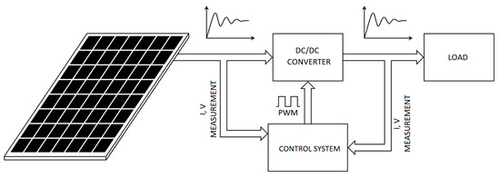
Figure 1.
Measurement system used for testing MPPT algorithms.
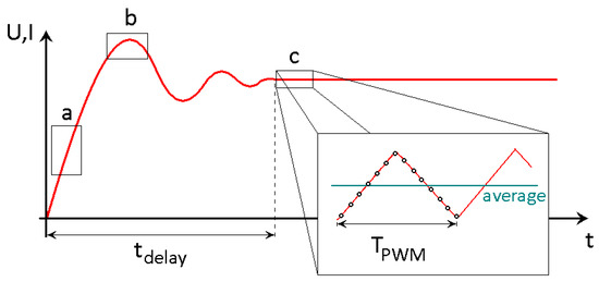
Figure 2.
An example of a signal on the input/output of a converter and a measurement obtained a—below the average value, b—above the average value and c—at the average value in quiescent region.
During the measurements, the total number of samples was adjustable. The goal was to find the minimum number of samples for a given sample ratio that ensures repeatability and relatively high accuracy of the measurements. Additionally, the acquisition of the samples over a larger number of switching periods in general improves the signal-to-noise ratio [29], which has a positive impact on the accuracy and repeatability of the system. The final parameter that was changed during the measurements was the time delay, tdelay (Figure 2), which introduces a time gap between the change in the duty cycle and the measurement itself. The introduction of the delay enabled measurements at different points in time on the transient curve (a–c in Figure 2).
Figure 2 shows how the measurement was performed. If the number of samples was relatively small in comparison to the transient time (e.g., 14 samples corresponding to one switching cycle), the measurement included only a small part of the waveform. Therefore, when the ADCs measured the voltages and the currents at the rising edge (a in Figure 2), the final result would be expected to be smaller than the average value in the steady state (c in Figure 2). However, if the measurement was taken during the overshoot (b in Figure 2), the resulting value would be expected to be larger than it is in the steady state. Figure 3a,b shows the results of the measurements that included 14 and 140 samples, respectively, and that were taken at different points in time (with different delays). Figure 4a,b shows the signals measured using an oscilloscope. The time base in Figure 4 was set to 200 µs/div. In Figure 4a, the current and voltage gains were set to 20 mA/div and 900 mV/div (with 9.6 V offset), respectively. As for Figure 4b, the current and voltage gains were set to 10 mA/div and 200 mV/div (with 2.16 V offset), respectively.
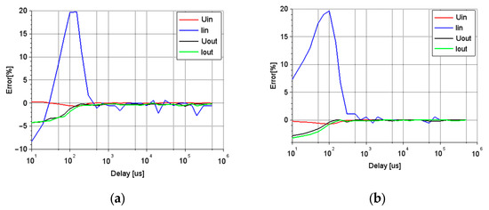
Figure 3.
Errors occurring in voltage and current measurements for different delays and the number of samples: (a) 14 samples corresponding to one switching cycle; (b) 140 samples corresponding to ten switching cycles.
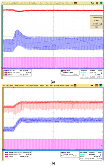
Figure 4.
Oscilloscope measurements of the (a) input signals and (b) output signals of a converter. The blue curves are currents, whereas the red curves are voltages. The purple curves represent the PWM signal.
It can be noticed that, during the measurements, the highest error existed in the first few hundred microseconds, which corresponds to the transients of the measured signals (Figure 4). Moreover, the largest overshoot is produced for the input current of the converter (blue line in Figure 4a), which indicates which signal measurement in this specific case is the most vulnerable to errors. Nevertheless, the error becomes smaller and the results become more stable after the signals reach a steady state. However, even in a steady state, the fluctuations can still reach a few percent. Figure 3b shows the same measurements but obtained using a higher number of samples; to be specific, it features 140 samples, which correspond to 10 switching periods of the PWM signal. The results are similar to the previous measurement except that, in the steady-state, the values are more consistent and stable: the maximum error for the larger number of samples, in the case of this measurement, reaches up to 0.5% of the steady-state value, which corresponds to a single-bit resolution. Including even larger numbers of samples improves the repeatability and reliability of the data; however, this increases the total acquisition time, which has an impact on the efficiency of the MPPT system. The whole measurement, including different signals, delays and the number of incorporated samples, is presented in the form of a 3D plane in Figure 5a–d.
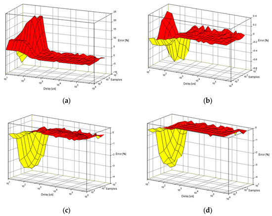
Figure 5.
Errors occurring in voltage and current measurements for different delays and the number of samples: (a) input current, (b) input voltage, (c) output current and (d) output voltage.
Data presented in Figure 5 show that transients can generate large errors during the measurement when a reasonable delay is not incorporated into the algorithm. It is clear that the error can be controlled with the measurement delay and the number of samples. The results show that acquiring samples from at least 10 switching periods is enough to obtain repeatable and reliable results. However, the samples should be taken within the steady state; otherwise, an error can occur. To show how the error can influence the maximum power point tracking, a power curve vs. the duty cycle has been drawn in Figure 6.
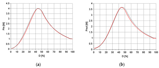
Figure 6.
Power characteristics measured in the peak error for the (a) power on the input of the converter and (b) power on the output of the converter. Continuous lines represent power measured in the steady state, while dashed lines represent power measured for the largest error.
The power curves were measured for the steady state (solid line), and the delay related to the highest error, which, in the case of the used converter, corresponded to 100 μs for the input power and 10 μs for the output power. It can be noticed that the power curves calculated for the highest error are shifted. This can cause an MPPT system to be working at a false maximum power point, which translates to a lower overall efficiency of the system. To measure voltages and currents in a steady state, one can determine the initial delay by using a small-signal model [30]. However, the transients can look differently for different duty cycles, especially in asynchronous converters and between continuous and discontinuous conduction modes (CCM, DCM); therefore, setting just one delay requires choosing the worst-case scenario, which often translates to a longer measurement time and thus lower efficiency of the system. Instead of setting a fixed delay, we propose an algorithm that automatically chooses the shortest delay that will not cause a shift in the power characteristics. It is based on the calculation of the difference between the previous and current measurements. The block diagram of the algorithm is presented in Figure 7.
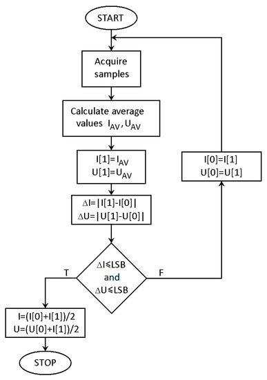
Figure 7.
Algorithm for finding steady-state values in transient signals.
Immediately after the perturbation of the duty cycle, the system measures the input/output currents and voltages. The measurements are taken at different points in time. Each measurement includes a number of samples, which should cover one or more switching cycles. Next, the samples are averaged, and the results are subtracted from the values acquired during the previous iteration. If the compared values differ just by one value that corresponds to the accuracy of the ADCs (for example, a less significant bit), then the algorithm averages the values from the current and previous iterations and returns them as steady-state values. In the case where the difference is larger, the current values take the place of the previous ones, and the process repeats itself, starting the next iteration.
3. Results and Discussion
To evaluate the algorithm of the measurement method presented in Figure 7, an experiment divided into two parts was performed. The purpose of the first part was to determine if the algorithm could reach the steady-state values of the current and voltage. Moreover, its purpose was to determine if it could reach the value faster than the algorithm with a constant delay between the duty cycle change and the measurement. The purpose of the second part of the experiment was to evaluate whether the proposed measurement method would give the same results as the constant delay measurement. For the evaluation, the measurement system presented in Figure 8 was used. A detailed description of the system can be found in [28]. The system ensures the stability of the light irradiation and enables voltage and current measurements with good accuracy. The schematic of the converter is presented in Figure 9, whereas the parameters of the converter as well as the parameters of the used PV panel are presented in Table 1.
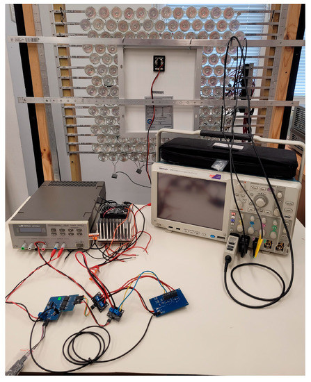
Figure 8.
The measurement setup used for evaluation of the proposed method.
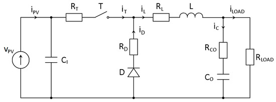
Figure 9.
Schematic of a buck converter.

Table 1.
Parameters of used devices.
3.1. Speed Evaluation
Because the time of the transients can be different for different quiescent values of the duty cycle, it is relevant to determine if the proposed measurement method can influence the total time to reach the maximum power point, which, as mentioned before, is one of the main factors that influence the efficiency of an MPPT algorithm. This is why, during the first part of the experiment, the proposed measurement method was implemented into a P&O algorithm and the time required to reach the MPP was measured. The search for the MPP starts by setting the duty cycle at 0.5% and is continued by increasing it by the same amount (i.e., 0.5%). During this time, the PWM signal and the PV panel output voltage were measured using the Tektronix MSO5104 oscilloscope. To obtain sufficient resolution, the sample rate of the oscilloscope was set to 50 MSPS. Figure 10 shows the results of the measurement. The lines at the top of the screen represent the PV output voltage, whereas the lines at the bottom of the screen represent the PWM signal. The time base in Figure 10 was set to 20 ms/div, whereas the voltage gains were set to 3.0 V/div.
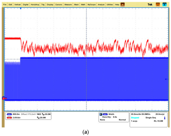
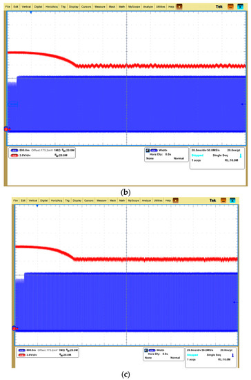
Figure 10.
Output voltage of a PV panel (red line) and PWM signal (blue line) during maximum power point searching while (a) the delay between the change in duty cycle and the measurement was equal to 10 μs, (b) the delay between the duty cycle change and the measurement was equal to 500 μs and (c) the delay was chosen automatically.
In Figure 10a, the delay was set to 10 μs, which is equivalent to a single switching cycle of the PWM signal. This measurement was made to show how the MPPT algorithm would perform in the case where the measurements of the current and voltage were taken during the transient time. The results show random oscillations with a high amplitude, which is not desirable in the MPPT system.
Figure 10b shows the PV voltage and PWM signals in the case where the currents and voltages were measured in the steady state (i.e., after 500 μs, according to Figure 3). The results show relatively small oscillations in the output voltage after the algorithm reaches the maximum power point, which occurs approximately after 50 ms for Da = 43%. In comparison, the algorithm with the proposed measurement method reached the maximum power point in 44 ms (Figure 10c), which is 12% faster than the measurement with the fixed delay. It is worth mentioning that, in both cases, the single measurement consisted of 140 samples, which corresponded to 10 switching cycles. This means that a single step in the MPPT algorithm took over one hundred microseconds plus the delay time. The number of samples was chosen based on the previous measurements (Figure 3b), according to which a smaller number of samples would lower the accuracy of the measurement. With lower accuracy, the MPPT algorithm features larger oscillations around the maximum power point, which has a negative impact on the efficiency of the MPPT system and thus should be avoided. Table 2 contains information on the standard deviation of the measured voltage at the maximum power point.
Table 2.
Deviation of the PV voltage.
Based on the data, it can be noticed that lowering the number of samples increases the deviation, which lowers the amount of energy extracted from a PV panel. On the other hand, the larger number of samples extends the total time of measurement, which also has a negative impact on the extracted power. What is interesting is that even though both of the used measurement methods featured the same number of samples, the measurement method that included automatic delay selection produced data with a smaller deviation. The difference in the standard deviation is not large, but it can be noticed that, in general, the results related to measurements with automatic delay selection feature a lower data deviation than measurements with a fixed delay.
3.2. Accuracy Measurement
This part of the experiment evaluated whether the proposed measurement method was accurate. To test the accuracy, we measured the power curve with the proposed measurement method and compared it with reference characteristics. The reason that the power characteristics were chosen is that, during measurement, the duty cycle changes throughout the whole range. Therefore, the currents and voltages experience different transients and thus provide different experiment conditions. To achieve reliable results, the reference power characteristics were measured with an initial delay equal to 1000 μs, whereas the number of samples was equal to 1400, which, in the case of the used system, was equivalent to 100 switching cycles. The proposed measurement method included 140 samples, which were equivalent to 10 switching cycles of the PWM signal. The measurements were taken for different irradiation levels using the measurement setup presented in Table 1. The results of the measurements are presented in Figure 11. The red lines represent the reference power curves, whereas the dashed lines refer to the proposed measurement with automatic delay selection. The difference between the MPP measured in the steady state (solid line) and the power measured using the proposed method (dashed line) in most cases did not exceed 0.2%. In one case, the difference was equal to 0.43%.
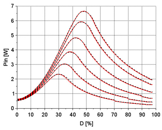
Figure 11.
Comparison of power curves measured at the input of the converter with a fixed delay (red line) and automatic delay (dashed line).
3.3. Discussion
The results presented in this section show that the proposed measurement method can reduce the time of a single measurement and thus reduce the total time to reach the maximum power point. The waveforms related to the proposed method seemed to be more consistent, which was confirmed by the numerical analysis. As for accuracy, it can be noticed that there is good consistency between the reference power curve and the characteristics measured with the proposed method. The differences between the curves become noticeable for small duty cycle values. Numerically, the maximum error between the curves was below 0.5% at the maximum power point. For the lower values of the duty cycle, the error was higher (for duty cycles below 12%, the error reached values above 5%). The larger error exists due to the resolution of the analog-to-digital converter, which can be increased by using an external AD converter or by incorporating oversampling [29,31]. The second idea would additionally extend the total time of a single measurement; therefore, using an external ADC with a higher resolution would be a preferable solution.
4. Conclusions
Time plays an important role in the total efficiency of a maximum power point tracking system; therefore, researchers working in the field of photovoltaics try to develop algorithms that will enable a relatively fast search for the maximum power point by the MPPT systems. However, the speed of an algorithm does not depend entirely on its structure but is limited by the transients of the converter used in the MPPT system. The existence of transients affects the way the signals of interest are going to be measured, i.e., to acquire accurate values of the relevant voltages and currents, the measurement should take place in a steady state. Otherwise, the measured values can experience deviations that can negatively influence the maximum power point tracking process, which was shown in the example of the P&O algorithm (Figure 10a). Moreover, the duration of the transients can be different depending on the quiescent value of the duty cycle, which can be especially observed in asynchronous converters and in the case of continuous and discontinuous conduction modes (CCM, DCM). Therefore, to ensure that the measurements are taken in a steady state, an appropriate delay between the change in the duty cycle and the measurement should be incorporated into the measurement system. The delay can be constant (chosen based on the worst-case scenario) or it can adapt to the duration of the transients. The method proposed in this paper, which includes the automatic selection of the delay, provides good accuracy and good consistency with the reference measurement that featured a constant delay. Moreover, the method can reduce the measurement time, which should have a positive impact on the efficiency of the MPPT algorithm. The used measurement setup featured larger errors for lower values of the duty cycle, which could be avoided in the future by incorporating one of the methods that would help to increase the ADCs’ resolution.
Author Contributions
Conceptualization, M.W. and L.B.; methodology, M.W. and L.B.; software, M.W.; validation, M.W. and L.B.; formal analysis, M.W. and L.B.; investigation, M.W. and L.B.; resources, M.W.; data curation, M.W.; writing—original draft preparation, M.W.; writing—review and editing, M.W. and L.B.; visualization, M.W.; supervision, M.W.; project administration, M.W. and L.B.; funding acquisition, M.W. and L.B. All authors have read and agreed to the published version of the manuscript.
Funding
This research received no external funding.
Data Availability Statement
Not applicable.
Conflicts of Interest
The authors declare no conflict of interest.
References
- Reisi, A.; Moradi, M.; Jamasb, S. Classification and Comparison of Maximum Power Point Tracking Techniques for Photovoltaic System: A Review. Renew. Sustain. Energy Rev. 2013, 19, 433–443. [Google Scholar] [CrossRef]
- Faranda, R.; Leva, S. Energy comparison of MPPT techniques for PV Systems. J. Electromagn. Anal. Appl. 2008, 3, 446–455. [Google Scholar]
- Esram, T.; Chapman, P.L. Comparison of Photovoltaic Array Maximum Power Point Tracking Techniques. IEEE Trans. Energy Convers. 2007, 22, 439–449. [Google Scholar] [CrossRef]
- Yilmaz, U.; Turksoy, O.; Teke, A. Improved MPPT method to increase accuracy and speed in photovoltaic systems under variable atmospheric conditions. Int. J. Electr. Power Energy Syst. 2019, 113, 634–651. [Google Scholar] [CrossRef]
- Podder, A.; Roy, N.; Pota, H. MPPT Methods for Solar PV Systems: A Critical Review Based on Tracking Nature. IET Renew. Power Gener. 2019, 13, 1615–1632. [Google Scholar] [CrossRef]
- Raghavendra, K.V.G.; Zeb, K.; Muthusamy, A.; Krishna, T.N.V.; Kumar, S.V.P.; Kim, D.H.; Kim, M.S.; Cho, H.G.; Kim, H.J. A Comprehensive Review of DC–DC Converter Topologies and Modulation Strategies with Recent Advances in Solar Photovoltaic Systems. Electronics 2020, 9, 31. [Google Scholar] [CrossRef]
- Jiang, J.A.; Huang, T.L.; Hsiao, Y.T.; Chen, C.H. Maximum Power Tracking for Photovoltaic Power Systems. J. Appl. Sci. Eng. 2005, 8, 147–153. [Google Scholar]
- Houssamo, I.; Locment, F.; Sechilariu, M. Experimental analysis of impact of MPPT methods on energy efficiency for photovoltaic power systems. Int. J. Electr. Power Energy Syst. 2013, 46, 98–107. [Google Scholar] [CrossRef]
- Mirhassani, S.M.; Razzazan, M.; Ramezani, A. An improved PSO based MPPT approach to cope with partially shaded condition. In Proceedings of the 2014 22nd Iranian Conference on Electrical Engineering (ICEE), Tehran, Iran, 20–22 May 2014; pp. 550–555. [Google Scholar]
- Kesilmis, Z.; Karabacak, M. Comparative study of maximum power point tracking algorithms under partial shading conditions. Istanb. Univ.—J. Electr. Electron. Eng. 2017, 17, 3335–3341. [Google Scholar]
- Mehazzem, F.; André, M.; Calif, R. Efficient Output Photovoltaic Power Prediction Based on MPPT Fuzzy Logic Technique and Solar Spatio-Temporal Forecasting Approach in a Tropical Insular Region. Energies 2022, 15, 8671. [Google Scholar] [CrossRef]
- Subramanian, V.; Indragandhi, V.; Kuppusamy, R.; Teekaraman, Y. Modeling and Analysis of PV System with Fuzzy Logic MPPT Technique for a DC Microgrid under Variable Atmospheric Conditions. Electronics 2021, 10, 2541. [Google Scholar] [CrossRef]
- Seddjar, A.; Kerrouche, K.; Wang, L. Simulation of the proposed combined Fuzzy Logic Control for Maximum Power Point Tracking and Battery Charge Regulation used in CubeSat. Arch. Electr. Eng. 2020, 69, 521–543. [Google Scholar]
- Chen, Y.T.; Jhang, Y.C.; Liang, R.H. A fuzzy-logic based auto-scaling variable step-size MPPT method for PV systems. Sol. Energy 2016, 126, 53–63. [Google Scholar] [CrossRef]
- Al-Mohaya, M.; Mahamad, A.; Saon, S. Implementation of Field Programmable Gate Array based Maximum Power Point Tracking controller of photovoltaic system. In Proceedings of the 2013 IEEE 7th International Power Engineering and Optimization Conference (PEOCO), Langkawi, Malaysia, 3–4 June 2013; pp. 718–721. [Google Scholar]
- Sankarganesh, R.; Thangavel, S. Maximum power point tracking in PV system using intelligence based PO technique and hybrid cuk converter. In Proceedings of the 2012 International Conference on Emerging Trends in Science, Engineering and Technology (INCOSET), Tiruchirappalli, India, 13–14 December 2012; pp. 429–436. [Google Scholar]
- Restrepo, C.; Yanẽz-Monsalvez, N.; González-Castaño, C.; Kouro, S.; Rodriguez, J. A Fast Converging Hybrid MPPT Algorithm Based on ABC and P&O Techniques for a Partially Shaded PV System. Mathematics 2021, 9, 2228. [Google Scholar]
- Karami, N.; Moubayed, N.; Outbib, R. General review and classification of different MPPT Techniques. Renew. Sustain. Energy Rev. 2017, 68, 1–18. [Google Scholar] [CrossRef]
- Brunton, S.; Rowley, C.; Kulkarni, S.; Clarkson, C. Maximum power point tracking for photovoltaic optimization using extremum seeking. In Proceedings of the 2009 34th IEEE Photovoltaic Specialists Conference (PVSC), Philadelphia, PA, USA, 7–12 June 2009; pp. 13–16. [Google Scholar]
- Lee, H.S.; Yun, J.J. Advanced MPPT Algorithm for Distributed Photovoltaic Systems. Energies 2019, 12, 3576. [Google Scholar] [CrossRef]
- Toumi, D.; Benattous, D.; Ibrahim, A.; Abdul-Ghaffar, H.I.; Obukhov, S.; Aboelsaud, R.; Labbi, Y.; Diab, A.A.Z. Optimal design and analysis of DC–DC converter with maximum power controller for stand-alone PV system. Energy Rep. 2021, 7, 4951–4960. [Google Scholar] [CrossRef]
- Femia, N.; Granozio, D.; Petrone, G.; Spagnuolo, G.; Vitelli, M. Predictive Adaptive MPPT Perturb and Observe Method. IEEE Trans. Aerosp. Electron. Syst. 2007, 43, 934–950. [Google Scholar] [CrossRef]
- Hayat, A.; Faisal, A.; Javed, M.Y.; Hasseb, M.; Rana, R.A. Effects of input capacitor (cin) of boost converter for photovoltaic system. In Proceedings of the 2016 International Conference on Computing, Electronic and Electrical Engineering (ICE Cube), Quetta, Pakistan, 11–12 April 2016; pp. 68–73. [Google Scholar]
- EN50530; Overall Efficiency of Grid Connected Photovoltaic Inverters. European Standard: Brussels, Belgium, 2010.
- Latham, A.M.; Sullivan, C.R.; Odame, K.M. Performance of photovoltaic maximum power point tracking algorithms in the presence of noise. In Proceedings of the 2010 IEEE Energy Conversion Congress and Exposition, Atlanta, GA, USA, 12–16 September 2010; pp. 632–639. [Google Scholar]
- Femia, N.; Petrone, G.; Spagnuolo, G.; Vitelli, M. Optimization of perturb and observe maximum power point tracking method. IEEE Trans. Power Electron. 2005, 20, 963–973. [Google Scholar] [CrossRef]
- Rico-Camacho, R.I.; Ricalde, L.J.; Bassam, A.; Flota-Bañuelos, M.I.; Alanis, A.Y. Transient Differentiation Maximum Power Point Tracker (Td-MPPT) for Optimized Tracking under Very Fast-Changing Irradiance: A Theoretical Approach for Mobile PV Applications. Appl. Sci. 2022, 12, 2671. [Google Scholar] [CrossRef]
- Walczak, M.; Bychto, L.; Kraśniewski, J.; Duer, S. Design and evaluation of a low-cost solar simulator and measurement system for low-power photovoltaic panels. Metrol. Meas. Syst. 2022, 29, 685–700. [Google Scholar]
- AN118: Improving ADC Resolution by Oversampling and Averaging; Silicon Labs: Austin, TX, USA, 2013.
- Janke, W.; Baczek, M.; Kraśniewski, J.; Walczak, M. Input Small-Signal Characteristics of Selected DC–DC Switching Converters. Energies 2022, 15, 1924. [Google Scholar] [CrossRef]
- AVR121: Enhancing ACD Resolution by Oversampling; Microchip Technology: Chandler, AZ, USA, 2005.


Disclaimer/Publisher’s Note: The statements, opinions and data contained in all publications are solely those of the individual author(s) and contributor(s) and not of MDPI and/or the editor(s). MDPI and/or the editor(s) disclaim responsibility for any injury to people or property resulting from any ideas, methods, instructions or products referred to in the content. |
© 2023 by the authors. Licensee MDPI, Basel, Switzerland. This article is an open access article distributed under the terms and conditions of the Creative Commons Attribution (CC BY) license (https://creativecommons.org/licenses/by/4.0/).