Operation Control Method for High-Speed Maglev Based on Fractional-Order Sliding Mode Adaptive and Diagonal Recurrent Neural Network

Abstract

The speed profile tracking calculation of high-speed maglev trains is mainly affected by running resistance. In order to reduce the adverse effects and improve tracking accuracy, this paper presents a maglev train operation control method based on a fractional-order sliding mode adaptive and diagonal recurrent neural network (FSMA-DRNN). First, the kinematic resistance equation is established due to the three types of resistance that occur during the actual operation of a train: air resistance, guide eddy current resistance, and suspension frame generator coil resistance. Then, the FSMA-DRNN control law and parameter update law are designed, and a FSMA-DRNN operation controller is composed of three parts: speed feed forward, fractional-order sliding mode adaptive equivalent control, and diagonal recurrent neural network resistance compensation. Furthermore, by using the designed operation controller, it is proven effective by the Lyapunov theory for the stability of the closed-loop control system. Apart from the proposed theoretical analysis, the proposed approaches are verified by experiments on the high-speed maglev hardware-in-the-loop simulation platform Rt-Lab, in line with the 29.86 km test line and a five-car train from the Shanghai maglev, showing the effectiveness and superiority for operation optimization.

1. Introduction

A high-speed maglev transportation system adopts non-contact levitation and guidance technology, based on electromagnetic principles, is propelled by linear motors to drive trains, and is a high-speed green means of transportation [1,2]. High-speed maglev trains can reach over 300–600 km/h, whereas medium–low-speed maglev trains can only reach below 300 km/h. Different from wheel-rail transit systems, maglev trains are affected by various resistance factors such as slope, air resistance, the eddy current effect, and back electromotive force during operation [3,4,5]. In the operation control field of maglev transportation, it has become more and more difficult in recent years to reduce the impact of train running resistance, improve train speed tracking accuracy, and design high-performance train running controllers.

The operation controller is an important component of the maglev train Operation Control System (OCS), and the main task is to effectively and precisely track the optimized speed curve, to ensure operation actions such as automatic departure, acceleration, cruising, coasting, braking, and precise parking [6,7]. However, during the train running process, the location and speed states frequently change, and the acceleration and deceleration actions are contained in the continuous domain, which may result in enormous state space and dimension errors [8]. Thus, speed curve tracking involves vital steps to ensure that the optimal speed curve is energy-saving and provides anti-disturbance tracking control with high precision [9,10,11]. High-performance operation control algorithms can dynamically adjust actual operation curves based on line parameters, reduce the adverse impact of operation resistance, precisely track the preset speed profile, and improve train control quality.

In recent years, speed tracking algorithms have tended to mature for wheel rail transit systems, mainly including the classical control algorithm, parameter adaptive control algorithm, intelligent control algorithm, and integrated intelligent control algorithm. In [12,13], a multimodal fuzzy PID (MMFPID) control algorithm was proposed, which uses traction feed forward and local output limiting methods to improve the dynamic performance of the controller, achieving the fast tracking of the train speed target profile. In [14], an adaptive fuzzy sliding mode controller was designed to soften the nonlinear switching control signal and achieve accurate parking. In [15], the multi-step Kalman filter control was performed to overcome the control delay time and to realize a precise stop. In [16], a finite-time double sliding surface guidance (DSSG) algorithm for the subway speed profile tracking was developed, with the convergence proved by the theories. In [17], the method was based on the matter-element theory, and the corresponding function of the performance indices drawn on the speed trajectory was proposed. In [18,19], a model-free fuzzy PID controller was constructed, which was used to adaptively adjust the PID gains. In [20], a model free adaptive controller combined with a neural network and PID algorithm in order to realize adaptive control was designed. In [21,22,23], for subway train speed tracking with speed sensor fault and over-speed protection, a model free adaptive iterative learning control based on a fault-tolerant control (MFAILC-FTC) scheme was put forward. In [24], for the purpose of solving the speed and position tracking control based on the multiple-point-mass dynamic model, a radial basis function neural-network-based adaptive iterative learning fault-tolerant control algorithm (RBFNN-AILFTC) was utilized. In [25,26], a DRTO method to optimize train operations was proposed according to deep RL (Reinforcement Learning) techniques, addressing several challenges of the changes in running states and multiple trains. Q-learning was used in [27,28], and a deep Q-network (DQN) [29,30] was applied to optimize the set operation strategy, in which neural networks were applied to conduct the RL process. In [31], two smart train operation (STOD and STON) algorithms were proposed by integrating expert knowledge with reinforcement learning algorithms.

The experimental or simulation results of the above methods demonstrated that these controllers can converge within a certain period of time for a wheel/rail transit system, but they are not strictly suitable for occasions such as maglev trains being affected by magnetic operation resistance, for a low/medium-speed maglev train. In [32], a fractional-order sliding mode adaptive neural network on the basis of operation controller was executed, estimating and compensating for the running resistance of a medium-speed maglev train to meet the requirements for train control accuracy and robustness. In [33], a fractional-order PID-based operation control method was performed, tracking the target speed profile of the train and reducing the influence of various running resistances on running process. In [34], a periodic adaptive compensation controller was proposed, consisting of four parts: a PD module, a speed feed-forward module, a periodic adaptive learning line additional resistance compensator, and an eddy current resistance and air resistance compensator.

For tackling the problem of high-speed maglev train asymptotic tracking under unknown time-varying resistance or unknown parameters, such as actuator failures, this paper proposes the speed profile tracking method based on a fractional-order sliding mode adaptive and diagonal recurrent neural network (FSMA-DRNN). Fractional-order sliding mode controllers provide robustness to disturbances and uncertainties [35], and diagonal recurrent neural networks offer adaptability to system changes [36,37].

The rest of this article is organized as follows. Section 2 describes the dynamic model of a high-speed maglev train. Section 3 formulates the computation model of a FSMAC-DRNN operation controller, the design of the control law of this controller, and how the stability is proven. Simulations are carried out in Section 4 by using the Shanghai maglev line scenario to validate the proposed approach. Finally, the conclusion and some discussion are provided in Section 6.

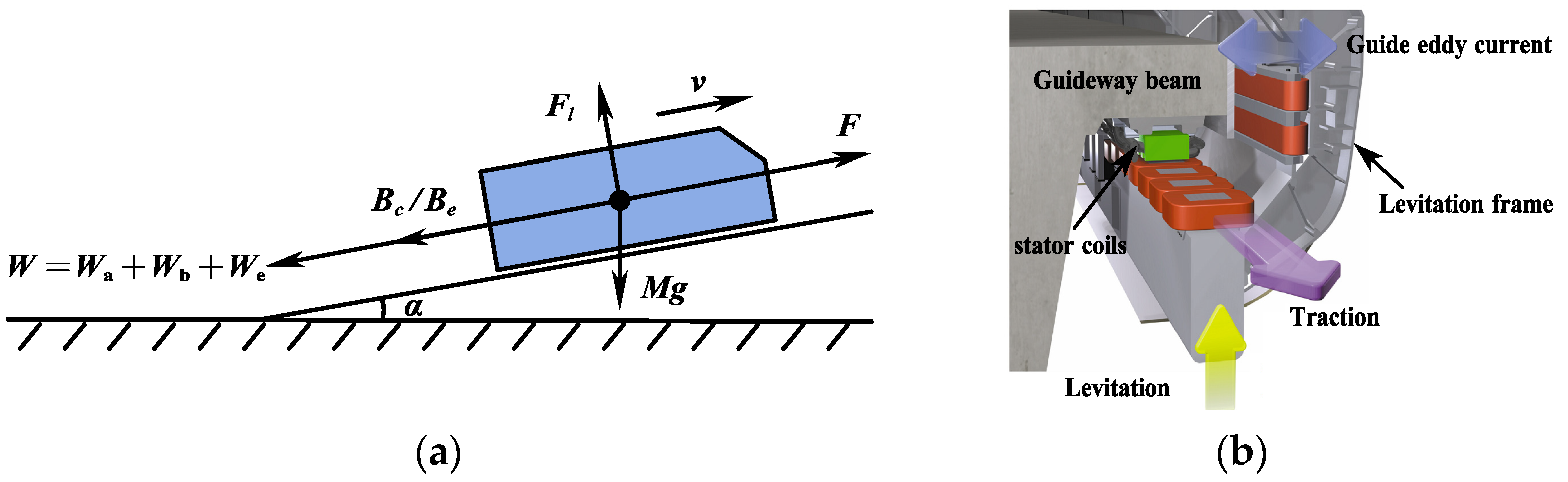
2. Dynamic Model of High-Speed Maglev Train

On the basis of Newton’s laws of motion, the dynamic equation of a high-speed maglev train is established:

$$ma=F_p-B-W.$$

(1)

F_p is the traction force, generated by a long stator linear synchronous motor; B is the braking force, produced by the eddy current braking system and the skid; W is the running resistance of the train, consisting of air resistance and additional resistance; m is the train mass; and a is the train acceleration. If the control output is F(t) = F_p, then B(t) and W(t) represent the electromagnetic and mechanical resistance at time t, respectively, and the kinematic model of the train is as follows [16]:

$$\begin{array}{l}\dot{x}=v\\ a=\dot{v}=\frac{1}{m}[F(t)-B(t)-W(t)]\end{array}.$$

(2)

X is the displacement of the maglev train, and v is the velocity. $\dot{x}$ and $\dot{v}$ represent the differentiation of x and v, respectively. The force analysis of a single mass model for the maglev train is shown in Figure 1.

2.1. Tractive Force Model

The tractive force of the maglev train is provided by the long stator synchronous linear motor; ${\psi }_d$, ${\psi }_q$, $i_d$, $i_q$ are the magnetic linkage and current components of the stator winding on the d-q axis, respectively; and $\tau$ is the stator pole distance. According to the rotor magnetic field-oriented control strategy, $i_d$ is usually controlled to 0, and the model is described as follows [11,38]:

$$F=\frac{3\pi }{2\tau }({\psi }_d\times i_q-{\psi }_q\times i_d)\stackrel{ i_d=0 }{\to }F=\frac{3\pi }{2\tau }·{\psi }_d\times i_q.$$

(3)

2.2. Braking Force Model

The braking force consists of a conventional braking force B_c and an emergency braking force B_e. The conventional braking force is created by the long stator linear motor, that is, the tractive force is reversed. The emergency braking force is generated by the eddy current effect between the lateral braking magnetic pole and the guideway and is expressed by [11,39]

$$B_c=F=\frac{3\pi }{2\tau }({\psi }_d\times i_q-{\psi }_q\times i_d),$$

(4)

$$B_e=\{\begin{array}{ll}q·1.2m·(1-e^{(-v/v_c)})\hfill & (v\ge 2.78\mathrm{m}/\mathrm{s})\\ \mu ·mg·\sqrt{1-{\left(\frac{x}{1000}\right)}^2}\hfill & (0<v<2.78\mathrm{m}/\mathrm{s})\\ 0\hfill & (v=0)\end{array}.$$

(5)

where q represents the eddy current braking level, v_c is the speed constant, and μ is the friction coefficient.

2.3. Running Resistance Model

The running resistance is mainly composed of air resistance W_a, guideway eddy current resistance W_e, and the resistance W_b generated by the harmonics of the linear generator on the suspension frame that hinders the relative movement of the traveling wave magnetic field. The specific expression is as follows [40,41,42]:

$$W_a=(W_x·v^2)·{10}^{-3},$$

(6)

$$W_e=n·0.5·[{(v/111)}^{0.7}+1.3·{(v/111)}^{0.7}],$$

(7)

$$W_b=\{\begin{array}{ll}n·(146/v-0.2)\hfill & (v\ge 41.7\mathrm{m}/\mathrm{s})\\ n·3.3\hfill & (5.56<v<41.7\mathrm{m}/\mathrm{s})\\ 0\hfill & (0<v<5.56\mathrm{m}/\mathrm{s})\end{array}.$$

(8)

where n represents the number of wagons, and W_x represents the air resistance coefficient during the running.

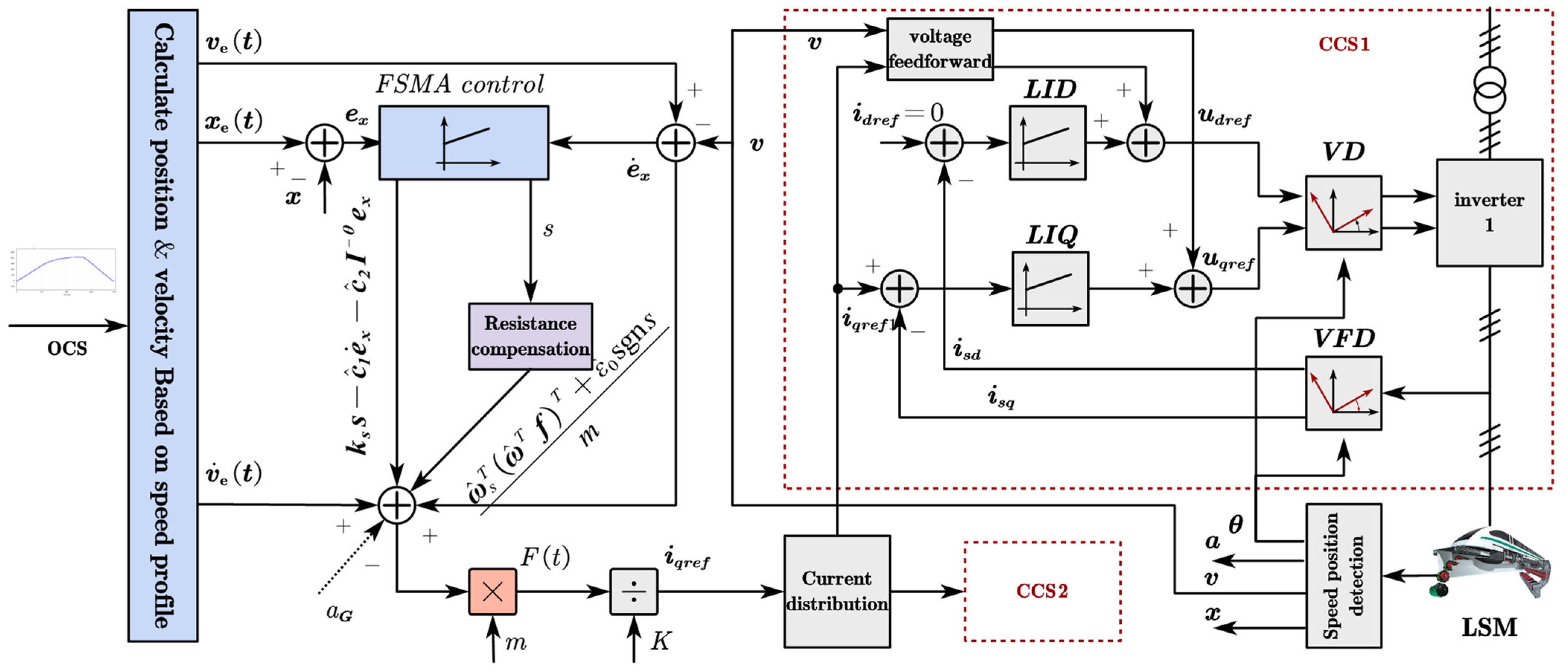
3. FSMA-DRNN Operation Controller Design

In order to minimize the impact of running resistance on the train position and speed tracking control and improve the running control performance of high-speed maglev trains, an operation controller based on a fractional-order sliding mode adaptive diagonal recurrent neural network is developed by combining three algorithms: fractional-order control, sliding mode adaptive control, and a diagonal recurrent neural network. Under the premise of ensuring the stability of the controller, the diagonal recurrent neural network is used to estimate the running resistance and the fractional-order adaptive sliding surface to ensure that the adaptive algorithm has a larger adjustment interval.

3.1. FSMA-DRNN Control Law

The position and speed error of high-speed maglev train are given as

$$e_x=x-x_e(t),$$

(9)

$${\dot{e}}_x=\dot{x}-{\dot{x}}_e(t)=v-v_e(t).$$

(10)

where e_x is the actual displacement error, x_e(t) is the expected displacement distance, $v_e(t)$ is the expected velocity, and ${\dot{v}}_e(t)$ is the expected acceleration. It is assumed that the parameters and disturbances are uncertain, but the system is bounded.

$$s={\dot{e}}_x+c{e}_x,$$

(11)

$$s={\dot{e}}_x+{\hat{c}}_1{e}_x+{\hat{c}}_2{D}^{\theta -1}{e}_x.$$

(12)

The design of the adaptive law for sliding mode control is shown in Equation (11), and the fractional-order error is introduced in Equation (12), where ${\hat{c}}_1$ is the sliding mode adaptive parameter, ${\hat{c}}_2$ is the fractional-order adaptive parameter, D is a differential operator, and $\theta -1$ is the differential order between 1 and 2.

Considering the ability of neural networks to fit unknown nonlinear functions, this paper adopts diagonal recurrent neural networks (DRNNs) to estimate and compensate train running resistance. A DRNN is similar to a feedforward network and consists of three key parts: an input layer, a hidden layer, and an output layer. The difference lies in that each neuron in the hidden layer has a self-feedback loop, making it simple in structure and easy to use for constructing training, as shown in Figure 2. The self-feedback weight W(t) can be written as

$$\{\begin{array}{l}W(t)={\mathit{\omega }}_s^T{({\mathit{\omega }}^{T}f(\lambda (t)))}^T+\mathit{\epsilon }(\lambda (t))\hfill \\ \mathit{f}(\lambda (t))=[f_1(\lambda (t),\dots ,f_p(\lambda (t)]\hfill \\ \lambda (t)={[e_x(t),\dots ,{\hat{e}}_x(t)]}^T\hfill \\ \begin{array}{l}\left|\epsilon (\lambda (t))\right|\le {\epsilon }_0\hfill \\ \mathit{\omega }\in R^p,{\mathit{\omega }}_s\in R^p,\mathit{f}(\lambda (t))\in R^p\hfill \end{array}\hfill \end{array}.$$

(13)

where p denotes the number of neurons; $\mathit{\omega }$ is the weight vector of the neural network; ${\mathit{\omega }}_s$ is the diagonal weight vector of hidden layer neurons; $\lambda (t)$ is the input vector; $\epsilon (t)$ is the error, which is bounded; and $\mathit{f}(\lambda (t))$ is the basis function of the neural network. The basis function of the k-th neuron can be expressed as a Gaussian function:

$$f_k(\lambda (t))=\exp \left[-\frac{{(\lambda (t)-{\lambda }_k)}^T(\lambda (t)-{\lambda }_k)}{2{\sigma }_k^2}\right](k=1,2,\dots p).$$

(14)

where ${\lambda }_k$ is the center of the k-th neuron, and ${\sigma }_k$ is the width. The estimated running resistance value $\hat{W}$ is

$$\hat{W}={\hat{\mathit{\omega }}}_s^T{({\hat{\mathit{\omega }}}^T\mathit{f}(\lambda (t)))}^T.$$

(15)

$\hat{\mathit{\omega }}$ and ${\hat{\mathit{\omega }}}_s$ are the estimated values of the forward and diagonal weights, respectively. According to Equations (13) and (15), the estimation errors of the DRNN parameters are

$${\tilde{\mathit{\omega }}}_s^T={\mathit{\omega }}_s^T-{\hat{\mathit{\omega }}}_s^T$$

(16)

$${\tilde{\mathit{\omega }}}^T={\mathit{\omega }}^T-{\hat{\mathit{\omega }}}^T$$

(17)

$${\tilde{\epsilon }}_0={\epsilon }_0-{\hat{\epsilon }}_0.$$

(18)

where $\tilde{\mathit{\omega }}$ and ${\tilde{\mathit{\omega }}}_s$ are the estimated errors of the forward and diagonal weights, and is the upper bound of the neural network estimated error $\epsilon (\lambda (t))$. For reducing the impact of running resistance on train running control, a fractional-order sliding mode adaptive diagonal loop neural network control law is designed. First, take the derivative of Equation (12) and make $k_{s}s=\frac{\partial s}{\partial x}$ to obtain

$$\frac{\partial s}{\partial x}=k_{s}s=\dot{v}-{\dot{v}}_e(t)+{\hat{c}}_1{\dot{e}}_x+{\hat{c}}_2{I}^{-\theta }{e}_x,$$

(19)

$$\dot{v}=k_{s}s+{\dot{v}}_e(t)-{\hat{c}}_1{\dot{e}}_x-{\hat{c}}_2{I}^{-\theta }{e}_x.$$

(20)

Then, substituting Equation (20) into Equation (2) of motion, it can be obtained that

$$F(t)=k_{s}sm+{\dot{v}}_e(t)m-{\hat{c}}_1{\dot{e}}_{x}m-{\hat{c}}_2{I}^{-\theta }{e}_{x}m+B(t)+W(t).$$

(21)

By substituting Equation (13) into the above equation, based on the Lyapunov theorem, the FSMC-DRNN control law is obtained:

$$F(t)=k_{s}sm+{\dot{v}}_e(t)m-{\hat{c}}_1{\dot{e}}_{x}m-{\hat{c}}_2{I}^{-\theta }{e}_{x}m+B(t)+{\hat{\mathit{\omega }}}_s^T{({\hat{\mathit{\omega }}}^T\mathit{f})}^T-{\hat{\epsilon }}_0\mathrm{sgn}s.$$

(22)

where $k_s$ is the negative parameter to be designed, and sgns is the symbolic function of s. The parameters in Equation (22) are updated in real time using adaptive update laws, and the FSMA-DRNN update laws are

$$\begin{array}{l}{\dot{\hat{c}}}_1=-s{e}_x\\ {\dot{\hat{c}}}_2=-s{D}^{\theta -1}{e}_x\\ \dot{\hat{\mathit{\omega }}}=-\mathit{\Lambda }{\mathit{f}}^T\mathit{s}\\ {\dot{\hat{\mathit{\omega }}}}_s=-\mathit{\Pi }{\mathit{f}}^T\mathit{s}\\ {\dot{\hat{\epsilon }}}_0=k_{\epsilon }s\mathrm{sgn}s\end{array}.$$

(23)

where $k_{\epsilon }$ is the positive parameter to be designed, and $\mathit{\Lambda }$ and $\mathit{\Pi }$ are the positive definite matrices to be designed.

3.2. Controller Structure Design Process

The designed operation controller structure is described in Figure 3. Six parts form the controller, which are the optimal speed profile calculated part; the speed feedforward part ${\dot{v}}_e(t)$, that is the main basis for the system transient response; the fractional-order sliding adaptive equivalent control part $k_{s}s-{\hat{c}}_1{\dot{e}}_x-{\hat{c}}_2{I}^{-\theta }{e}_x$, used to improve operational control accuracy and robustness; the diagonal recurrent neural network part $[{\hat{\mathit{\omega }}}_s^T{({\hat{\mathit{\omega }}}^T\mathit{f})}^T+{\hat{\epsilon }}_{0}s\mathrm{sgn}s]/m$, aiming to estimate the resistance and compensate the acceleration during running in real time; the gravity acceleration compensation part a_G, caused by slope; the traction control system part, converters CCS1 and CCS2, realizing the long stator linear motor control and train speed and position detection; and the feedback to the operation controller.

3.3. Stability Analysis of the Controller

To prove the stability of the proposed control system, the direct method of Lyapunov is used. First, the Lyapunov energy function is constructed:

$$V=\frac{1}{2}m{s}^2+\frac{1}{2}{\tilde{\mathit{\omega }}}^T{\mathit{\Lambda }}^{-1}\tilde{\mathit{\omega }}+\frac{1}{2}{\tilde{\mathit{\omega }}}_s{}^T{\mathit{\Pi }}^{-1}{\tilde{\mathit{\omega }}}_s+\frac{1}{2k_{\epsilon }}{\tilde{\epsilon }}_0^2{.}_{}$$

(24)

Differentiate Equation (24) and obtain

$$V=ms\dot{s}+{\tilde{\mathit{\omega }}}^T{\mathit{\Lambda }}^{-1}\dot{\hat{\mathit{\omega }}}+{\tilde{\mathit{\omega }}}_s{}^T{\mathit{\Pi }}^{-1}{\dot{\hat{\mathit{\omega }}}}_s+\frac{1}{k_{\epsilon }}{\tilde{\epsilon }}_0{\dot{\hat{\epsilon }}}_0.$$

(25)

The definition of the fractional-order integral is

$${}_{\alpha }I_t^{\alpha }=\frac{1}{\Gamma (\alpha )}{\displaystyle \underset{a}{\overset{t}{\int }}\frac{f(\tau )}{{(t-\tau )}^{1-\alpha }}}d\tau .$$

(26)

The definition of the fractional-order differential is

$${}_{\alpha }D_t^{\beta }=\frac{1}{\Gamma (n-\beta )}{\displaystyle \underset{a}{\overset{t}{\int }}\frac{f^{(n)}(\tau )}{{(t-\tau )}^{\beta -n+1}}}d\tau .$$

(27)

where ${}_{\alpha }I_t^{\alpha }$ is a fractional-order integral operator; ${}_{\alpha }D_t^{\beta }$ is a fractional-order differential operator; a and t are the upper and lower limits of the integral operator, respectively; $\alpha$ and $\beta$ represent the order of the integral and differential operators, respectively; $\Gamma (*)$ is the Euler Gamma functions; and n is an integer, even $n-1<\beta <n$.

Based on the fractional calculus properties in Equations (26) and (27), the rate of the sliding surface changes is obtained, replacing kinematic Equations (1) and (2) and sliding surface Equation (12):

$$\begin{array}{l}\dot{s}={\ddot{e}}_x+{\dot{\hat{c}}}_1{e}_x+{\hat{c}}_1{\dot{e}}_x+{\dot{\hat{c}}}_2{D}^{\theta -1}{e}_x+{\hat{c}}_2{I}^{-\theta }{e}_x\\ =\frac{1}{m}[F(t)-B(t)-W(t)-m{\dot{v}}_e(t)]+{\dot{\hat{c}}}_1{e}_x+{\hat{c}}_1{\dot{e}}_x+{\dot{\hat{c}}}_2{D}^{\theta -1}{e}_x+{\dot{\hat{c}}}_2{I}^{-\theta }{e}_x\end{array}.$$

(28)

Substitute Equations (22) and (28) into Equation (25) to obtain the derivative of the Lyapunov energy function:

$$\begin{array}{l}\dot{V}=ms\dot{s}-{\tilde{\mathit{\omega }}}^T{\mathit{\Lambda }}^{-1}\dot{\hat{\mathit{\omega }}}-{\tilde{\mathit{\omega }}}_s{}^T{\mathit{\Pi }}^{-1}{\dot{\hat{\mathit{\omega }}}}_s-\frac{1}{k_{\epsilon }}{\tilde{\epsilon }}_0{\dot{\hat{\epsilon }}}_0\\ =s[F(t)-B(t)-W(t)-m{\dot{v}}_e(t)]\\ +ms[{\dot{\hat{c}}}_1{e}_x+{\hat{c}}_1{\dot{e}}_x+{\dot{\hat{c}}}_2{D}^{\theta -1}{e}_x+{\dot{\hat{c}}}_2{I}^{-\theta }{e}_x]-{\tilde{\mathit{\omega }}}^T{\mathit{\Lambda }}^{-1}\dot{\hat{\mathit{\omega }}}-{\tilde{\mathit{\omega }}}_s{}^T{\mathit{\Pi }}^{-1}{\dot{\hat{\mathit{\omega }}}}_s-\frac{1}{k_{\epsilon }}{\tilde{\epsilon }}_0{\dot{\hat{\epsilon }}}_0\\ =s[k_{s}sm-{\hat{c}}_1{\dot{e}}_{x}m-{\hat{c}}_2{I}^{-\theta }{e}_{x}m+{\hat{\mathit{\omega }}}_s{}^T{({\hat{\mathit{\omega }}}^T\mathit{f})}^T-{\hat{\epsilon }}_0\mathrm{sgn}s-{\mathit{\omega }}_s^T{({\mathit{\omega }}^T\mathit{f})}^T-\epsilon (\lambda (t))]\\ +ms[{\dot{\hat{c}}}_1{e}_x+{\hat{c}}_1{\dot{e}}_x+{\dot{\hat{c}}}_2{D}^{\theta -1}{e}_x+{\dot{\hat{c}}}_2{I}^{-\theta }{e}_x]-{\tilde{\mathit{\omega }}}^T{\mathit{\Lambda }}^{-1}\dot{\hat{\mathit{\omega }}}-{\tilde{\mathit{\omega }}}_s{}^T{\mathit{\Pi }}^{-1}{\dot{\hat{\mathit{\omega }}}}_s-\frac{1}{k_{\epsilon }}{\tilde{\epsilon }}_0{\dot{\hat{\epsilon }}}_0\\ =k_s{s}^{2}m+s{\dot{\hat{c}}}_1{e}_{x}m+s{\dot{\hat{c}}}_2{D}^{\theta -1}{e}_{x}m+s{\hat{\mathit{\omega }}}_s{}^T{({\hat{\mathit{\omega }}}^T\mathit{f})}^T-s{\mathit{\omega }}_s{}^T{({\mathit{\omega }}^T\mathit{f})}^T-s{\hat{\epsilon }}_0\mathrm{sgn}s-s\epsilon (\lambda (t))\\ -{\tilde{\mathit{\omega }}}^T{\mathit{\Lambda }}^{-1}\dot{\hat{\mathit{\omega }}}-{\tilde{\mathit{\omega }}}_s^T{\mathit{\Pi }}^{-1}{\dot{\hat{\mathit{\omega }}}}_s-\frac{1}{k_{\epsilon }}{\tilde{\epsilon }}_0{\dot{\hat{\epsilon }}}_0\end{array}.$$

(29)

Due to $s{\hat{\epsilon }}_0\mathrm{sgn}s-s\epsilon (\lambda (t))\le s{\hat{\epsilon }}_0\mathrm{sgn}s$, Equation (29) can be simplified as follows:

$$\begin{array}{l}\dot{V}\le k_s{s}^{2}m+s{\dot{\hat{c}}}_1{e}_{x}m+s{\dot{\hat{c}}}_2{D}^{\theta -1}{e}_{x}m-s{\tilde{\mathit{\omega }}}_s^T{\mathit{f}}^T-s{\tilde{\mathit{\omega }}}^T{\mathit{f}}^T+s{\hat{\epsilon }}_0\mathrm{sgn}s\\ -{\tilde{\mathit{\omega }}}^T{\mathit{\Lambda }}^{-1}\dot{\hat{\mathit{\omega }}}-{\tilde{\mathit{\omega }}}_s^T{\mathit{\Pi }}^{-1}{\dot{\hat{\mathit{\omega }}}}_s-\frac{1}{k_{\epsilon }}{\tilde{\epsilon }}_0{\dot{\hat{\epsilon }}}_0\\ \dot{V}\le k_s{s}^{2}m+s{\dot{\hat{c}}}_1{e}_{x}m+s{\dot{\hat{c}}}_2{D}^{\theta -1}{e}_{x}m-{\tilde{\mathit{\omega }}}_s^T(s{\mathit{f}}^T+{\mathit{\Lambda }}^{-1}\dot{\hat{\mathit{\omega }}})\\ -{\tilde{\mathit{\omega }}}^T(s{\mathit{f}}^T+{\mathit{\Pi }}^{-1}{\dot{\hat{\mathit{\omega }}}}_s)+{\tilde{\epsilon }}_0(s\mathrm{sgn}s-\frac{1}{k_{\epsilon }}\dot{\hat{\epsilon }})\end{array}.$$

(30)

Substitute Equation (23) into Equation (30) to obtain

$$\dot{V}\le k_s{s}^2-s^2{e}_x^{2}m-{(s{D}^{\theta -1}{e}_x)}^{2}m-{\tilde{\mathit{\omega }}}_s{}^T(s{\mathit{f}}^T+{\mathit{\Lambda }}^{-1}\dot{\hat{\mathit{\omega }}}).$$

(31)

where $k_s$ is a negative parameter, and $\dot{V}\le 0$. According to the Lyapunov stability theorem, $s$, $\hat{\mathit{\omega }}$, ${\hat{\mathit{\omega }}}_s$ and ${\hat{\epsilon }}_0$ are bounded when the time tends to infinity, the error converges to 0, and the system asymptotic stabilizes, indicating that the designed FSMA-DRNN controller can ensure the operation control of high-speed maglev trains.

4. Experimental Verification

Experimental verification was conducted based on the high-speed maglev hardware-in-the-loop simulation system platform Rt-Lab, to validate the performance of the designed FSMA-DRNN controller, and the control performance was compared with that of the PID operating controller.

4.1. Test Line and Train Parameters

4.1.1. Line Parameter

The main line length is designed to be 29.86 km, in which the number of curves is 6, the number of slopes is 7, the maximum curve radius is 7997 m, the minimum curve radius is 1292 m, and the maximum slope is −1.076%. The curve accounts for 62% of the total length of the line, and the average slope section is 14.3%. The specific parameters are exhibited in

Table 1. Curve elements of hardware-in-the-loop simulation.

Parameters	Value
Total length of main line (km)	29.86
Number of curves	6
Curve line extension (km)	18.51
Curve in the total line (%)	62.0
Maximum curve radius (m)	7997.45
Minimum curve radius (m)	1292.52
Maximum transition curve (m)	2399.32
Minimum transition curve (m)	290.00

and

Table 2. Vertical section and slope elements of hardware-in-the-loop simulation.

Parameters	Value
Total number of slope sections	7
Average slope section length (km)	4.28
Average slope section length in total line length (%)	14.3
Maximum slope (%)	−1.076
Maximum slope length (m)	14,105.55
Minimum slope length (m)	650.55
Maximum vertical curve radius (m)	80,000
Minimum vertical curve radius (m)	45,000
Maximum transition curve (m)	100
Minimum transition curve (m)	20

.

4.1.2. Train Parameters

The train is a five-car formation, with an empty mass of 52.9 t at the head and tail, an empty mass of 50.3 t at the middle, and a total mass of 342.5 t. When accelerating, the maximum acceleration is 1 m/s², and, when decelerating, the maximum acceleration is 1.25 m/s². The maximum speed of the train reaches 430 km/h, and the train operation time is 465 s. The specific parameters of the vehicle are expressed in

Table 3. Train elements of hardware-in-the-loop simulation.

Parameters	Value
Formation/car	5, (2 head/tail, 3 middle)
Head/tail car—no-load weight (t)	52.9
Middle car—no-load weight (t)	50.3
Head/tail car—maximum allowable gross weight (t)	67.0
Middle car—maximum allowable gross weight (t)	69.5
Total weight of train (t)	342.5
Maximum speed (km/h)	430
Maximum acceleration during acceleration (m/s2)	1
Maximum acceleration during deceleration (m/s2)	12.5

.

4.2. Controller Parameter Setting

4.2.1. FSMA-DRNN and PID Control Parameter Setting

For the FSMA-DRNN controller under ideal conditions, based on the characteristics of the maglev train, the attenuation curve method can be used, which is combined with the trial-and-error method to tune the parameters. The fractional-order parameters are adjusted for the purpose of improving the control accuracy and robustness. For the PID operation controller, considering the rapidity and stability of the system, the critical proportionality method is applied to tune the proportional, integral, and differential gains. The parameters after setting are depicted in

Table 4. FSMA-DRNN and PID control parameters.

Controller	Parameter	Values
FSMA-DRNN	ks, θ	−397, 2.59
PID	kp, ki, kd	1200, 1310, 1

.

4.2.2. Adaptive Control Parameter Setting

Adaptive parameters affect the convergence speed of the system. If the parameters are too small, the convergence speed becomes slow, but if they are too large, overcorrection can easily occur, leading to system instability. Therefore, it is necessary to use the empirical method and the trial-and-error method to tune the adaptive parameters founded on the above parameter settings, while also taking into account relevant factors such as operating resistance. As a result, the setting parameters values are $k_{\epsilon }=7.12\times {10}^{-2}$, $\mathit{\Lambda }=2.2\times {10}^6\mathit{E}$, and $\mathit{\Pi }=1.7\times {10}^3\mathit{E}$.

4.3. Experimental Platform

The experimental platform is shown in Figure 4, consisting of four parts: a propulsion Rt_Lab system, a signal conditioning system, a propulsion control system, and an operation control simulation system. The Rt_Lab system includes two parts, the target PC realizes CU, SSS, and LSM simulation, and the host PC realizes managerial control. The signal conditioning system converts analog into digital. The propulsion control system performs speed output control, which consists of MCU, CCU1, CCU2, and SSC. The proposed speed control algorithm is executed in the operation control simulation system [43]. The layout of the test guideway line is shown in Figure 5.

5. Comparison of Experimental Results

In accordance with the above experimental parameters, this section mainly compares and analyzes the control performance of the FSMA-DRNN and PID controllers in terms of position and speed tracking, tracking error, resistance compensation, and traction control output. The single-direction simulation running time is 465 s, and the simulation time step is 0.1 s.

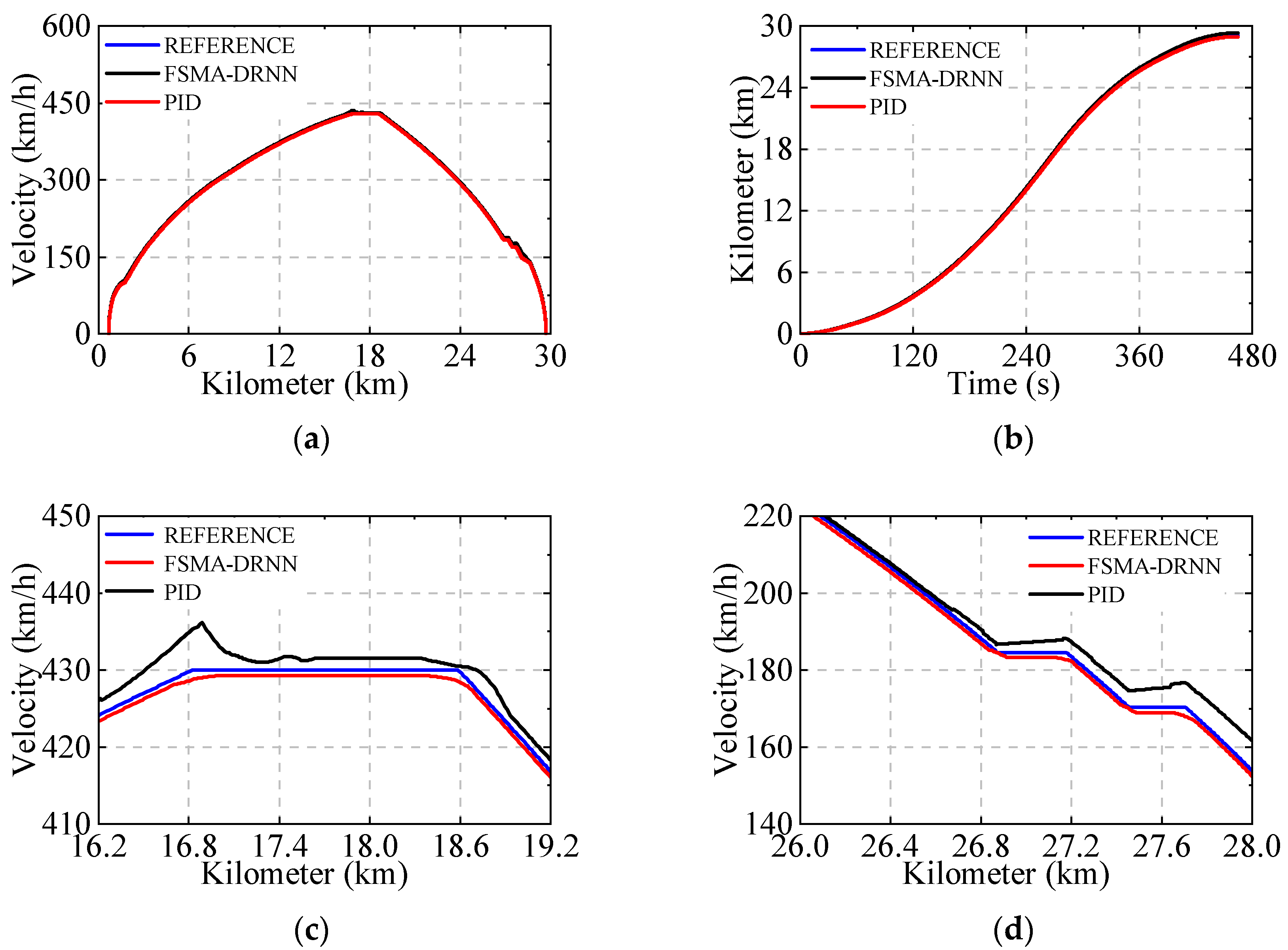
5.1. Comparison of Speed and Position Tracking Performance

The position and speed tracking effect of the FSMA-DRNN and PID operation controllers is clearly shown in Figure 6. The blue color is the preset optimal speed profile of the train, the black color is the PID control output, and the red color is the FSMA-DRNN control output. (a) refers to the overall speed tracking effect of the test line, (b) refers to the position tracking effect of the entire line, (c) refers to the tracking effect of the train accelerating to the maximum speed of 430 km/h, and (d) refers to the speed tracking effect during braking and deceleration. As shown in Figure 5, due to the FSMA-DRNN prediction and the compensation for running resistance, the tracking accuracy of FSMA-DRNN is higher than that of PID controllers, especially on lines with abrupt changes in speed and running resistance, when the FSMA-DRNN’s tracking control is smoother.

5.2. Comparison of Speed and Position Tracking Errors

As shown in Figure 7, the maximum absolute value of the speed tracking error for the PID controller reaches 8 km/h, and the maximum position tracking error reaches 2.6 m, while the maximum value tracking error for FSM-DRNN is controlled at 2.5 km/h and 0.35 m. The mean squared error of PID is much greater than that of FSMA-DRNN, especially for speeds around 150 km/h or positions around 3 km.

5.3. Estimated Effect of Running Resistance

In Figure 8, the blue line indicates the planar eddy current effect resistance between the guide magnetic pole and the longitudinal guideway, with the minimum resistance value; the orange line represents the air resistance—the main component of train running resistance, showing the increase in speed; the purple line indicates the electromagnetic resistance generated by the linear generator on the suspension frame, and, when the speed is less than 20 km/h, the resistance is zero, but, when the resistance is a constant value of 16.5 kN at 20–150 km/h, the resistance gradually decreases above 150 km/h. The black curve stands for the running resistance curve of the train during actual operation. The red curve represents the estimated running resistance of FSMA-DRNN, which is firstly almost consistent with the actual running resistance curve, and then slightly lower than the actual resistance during the sudden change part of the resistance, but it can be followed quickly afterward.

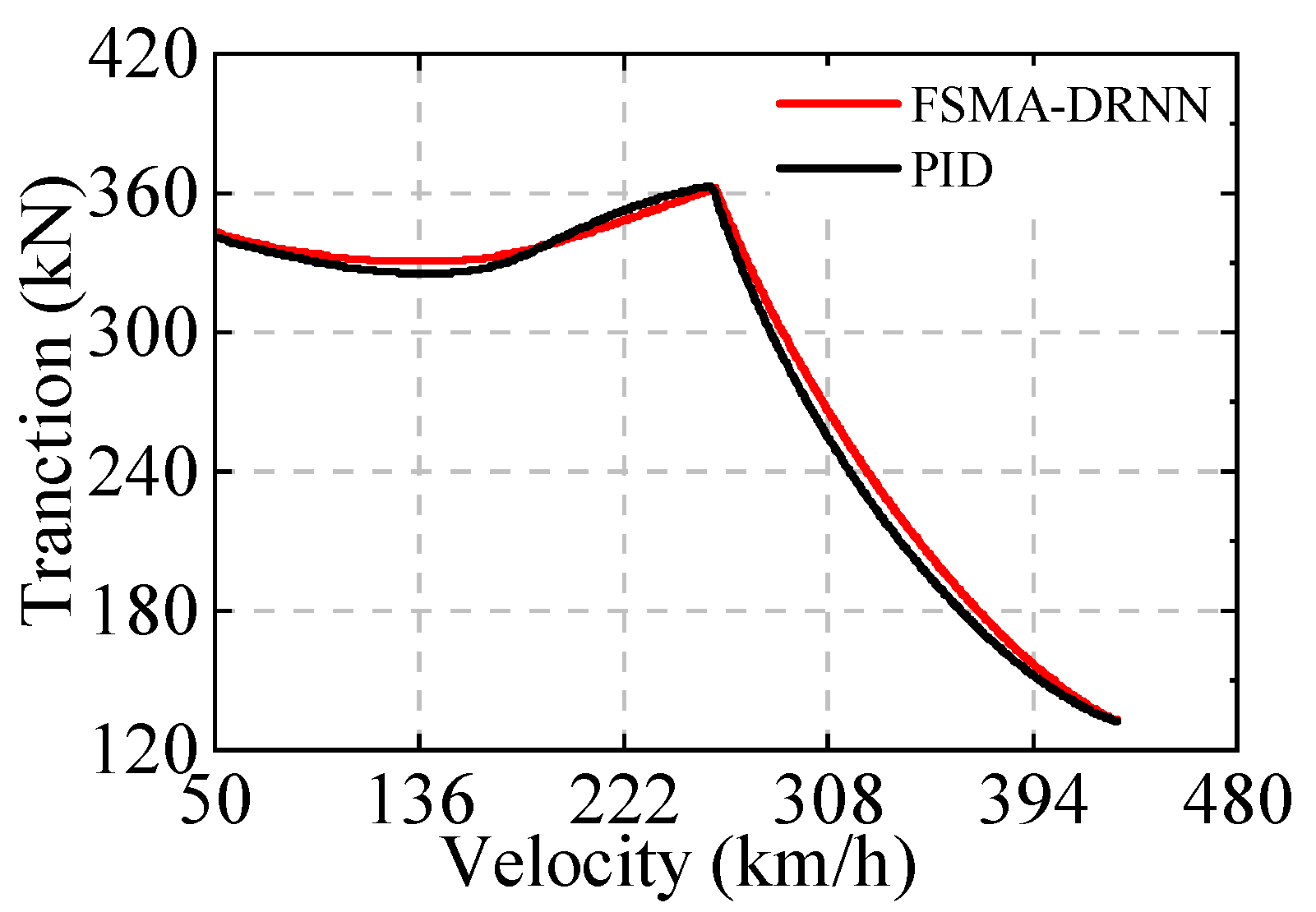
5.4. Comparison of Tractive Force Output Effects

As shown in Figure 9, due to the estimated compensation for operating resistance, the tractive force output of FSMA-DRNN is slightly higher than that of the PID controller at the same speed, but the output of FSMA-DRNN is smoother. When the train is running at 300 km/h, the maximum output is 360 KN; when the train is running at 430 km/h, the minimum output of the train is 135 kN. For the overall range, the tractive force output trends of the two controllers are consistent.

6. Conclusions

This paper studies the optimal speed profile tracking for a high-speed maglev train. The key conclusions and contributions of this work can be summarized as follows:

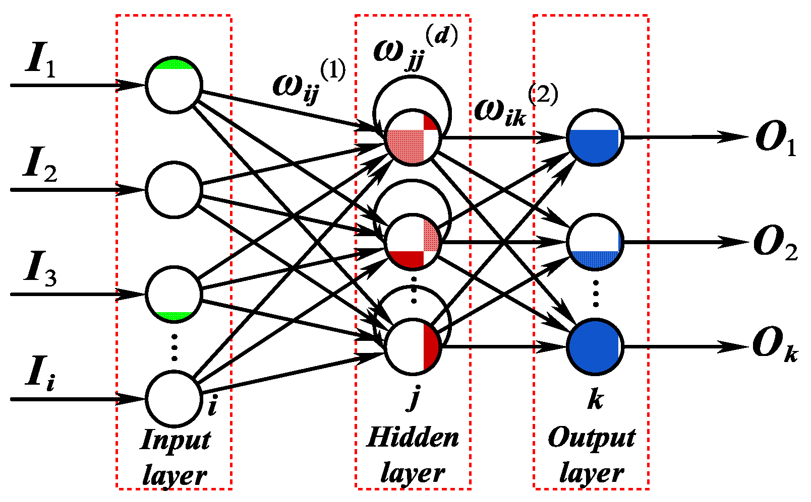
• A kinematics model for neural network recognition is established based on adopting the tractive force, braking force, and running resistance. A novel algorithm called DRNN is presented to predict the resistance for compensating for the output acceleration.
• A new fractional-order sliding mode adaptive control algorithm (FSMA) is proposed to track the optimal speed profile. By using the corresponding traction generated by FSMA, the speed profile can be tracked more effectively and robustly.
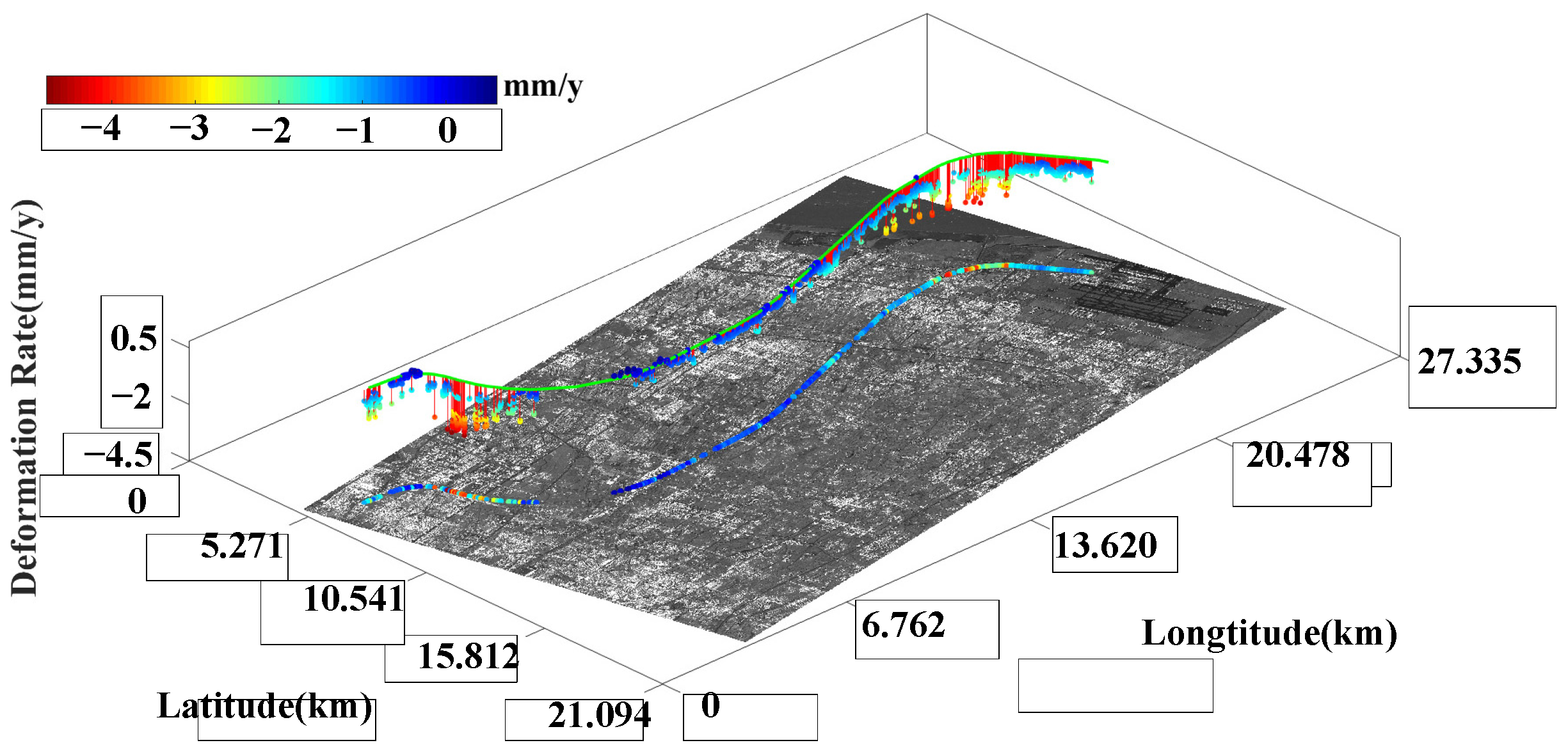
• The real data sets from the Shanghai maglev line are used on a hardware-in-the-loop platform for experimental simulations. Comparative studies for different control strategies validate the effectiveness and superiority of the proposed operation controller.

Note that for those maglev lines with unique scenarios and running characteristics, the tracking controller parameter proposed in the paper should be tuned accordingly. Thus, more extensive tests should be performed to enhance the universality of the proposed controller, which is an issue for future work.

References

1. Ding, S. 600 Km/h High-Speed Maglev Transportation System; Shanghai Scientific & Technical Publishers: Shanghai, China, 2022. [Google Scholar]
2. Wu, X. Maglev Train; Shanghai Scientific & Technical Publishers: Shanghai, China, 2003. [Google Scholar]
3. Gang, L.; Zhi, R.; Cui, L.; Zhang, Z.; Liu, Y. Analysis on the Air-Gap Magnetic Flux Density and Propulsion of the TFLSM Considering Cogging Effect. IEEE Trans. Magn. 2023, 59, 1–7. [Google Scholar]
4. Liao, Z.; Yue, J.; Lin, G. Application Research of HTS Linear Motor Based on Halbach Array in High Speed Maglev System. IEEE Trans. Appl. Supercond. 2021, 31, 1–7. [Google Scholar] [CrossRef]
5. Zhao, Y.; Peng, F.; Ren, L.; Lin, G.; Xu, J. A Levitation Condition Awaeness Architecture for Low-Speed Maglev Train Based on Data-Driven Random Matrix Analysis. IEEE Access 2020, 8, 176575–176587. [Google Scholar] [CrossRef]
6. Chen, C.; Xu, J.; Sun, Y.; Zhao, X. Sliding Mode Bifurcation Control Based on Acceleration Feedback Correction Adaptive Compensation for Maglev Train Suspension System With Time-Varying Disturbance. IEEE Trans. Transp. Electrif. 2022, 8, 2273–2287. [Google Scholar] [CrossRef]
7. Chen, C.; Xu, J.; Rong, L.; Ji, W.; Lin, G.; Sun, Y. Neural-Network-State-Observation-Based Adaptive Inversion Control Method of Maglev Train. IEEE Trans. Veh. Technol. 2022, 71, 3660–3669. [Google Scholar] [CrossRef]
8. Zhang, W.; Xu, Z.; Sun, M. Design of a Novel Claw Pole Transverse Flux Permanent Magnet Motor Based on Hybrid Stator Core. IEEE Trans. Magn. 2021, 57, 1–5. [Google Scholar] [CrossRef]
9. Xu, Y.; Zhao, X.; Yin, S.; Long, Z. Real-Time Performance Optimization of Electromagnetic Levitation Systems and the Experimental Validation. IEEE Trans. Ind. Electron. 2023, 70, 3035–3044. [Google Scholar] [CrossRef]
10. Jiang, S.; Xu, H.; Zhang, T.; Yao, X.; Long, Z. Lazy Prescribed-Time Synchronization Control of Half Bogie for High-Speed Maglev Train Considering Track Irregularities and Input Constraints. IEEE Trans. Veh. Technol. 2022, 71, 6924–6937. [Google Scholar] [CrossRef]
11. Lv, G.; Cui, L.; Zhi, R.; Zhou, T.; Liu, Y. Investigation of the Transverse Flux Linear Synchronous Motor Integrated with Propulsion, Levitation and Guidance for the Maglev Train. IEEE Trans. Transp. Electrif. 2023, 1. [Google Scholar] [CrossRef]
12. Yang, J.; Jia, L.; Lu, S.; Li, Z. Energy-efficient Operation of Electric Freight Trains-Part I: Speed Profile Optimization. J. China Railw. Soc. 2016, 38, 22–31. [Google Scholar]
13. Yang, J.; Jia, L.; Fu, Y.; Luo, Y. Energy-efficient Freight Train Operation-Part II: Combined Control of Speed Tracking. J. China Railw. Soc. 2016, 38, 23–31. [Google Scholar]
14. He, H.; Yang, Z.; Lv, J. Braking Control Algorithm for Accurate Train Stopping Based on Adaptive Fuzzy Sliding Mode. China Railw. Sci. 2019, 40, 122–129. [Google Scholar]
15. Kim, J.; Park, J.; Eun, Y. Precise Stop Control and Experimental Validation for Metro Train Overcoming Delays and Nonlinearities. IEEE Trans. Veh. Technol. 2022, 71, 4776–4787. [Google Scholar] [CrossRef]
16. Cao, Y.; Wang, C.; Liu, F.; Li, P.; Xie, G. Bio-Inspired Speed Curve Optimization and Sliding Mode Tracking Control for Subway Trains. IEEE Trans. Veh. Technol. 2019, 68, 6331–6342. [Google Scholar] [CrossRef]
17. Meng, J.; Xu, R.; Li, D.; Chen, X. Combining the Matter-Element Model With the Associated Function of Performance Indices for Automatic Train Operation Algorithm. IEEE Trans. Intell. Transp. Syst. 2019, 20, 253–263. [Google Scholar] [CrossRef]
18. Pu, Q.; Zhu, X.; Liu, J.; Cai, D.; Fu, G.; Wei, D.; Sun, J.; Zhang, R. Integrated Optimal Design of Speed Profile and Fuzzy PID Controller for Train With Multifactor Consideration. IEEE Access 2020, 8, 152146–152160. [Google Scholar] [CrossRef]
19. Liu, Y.; Fan, K.; Ouyang, Q. Intelligent Traction Control Method Based on Model Predictive Fuzzy PID Control and Online Optimization for Permanent Magnetic Maglev Trains. IEEE Access 2021, 9, 29032–29046. [Google Scholar] [CrossRef]
20. Pu, Q.; Zhu, R.; Zhang, R.; Liu, J.; Cai, D.; Fu, G. Speed Profile Tracking by an Adaptive Controller for Subway Train Based on Neural Network and PID Algorithm. IEEE Trans. Veh. Technol. 2020, 69, 10656–10667. [Google Scholar] [CrossRef]
21. Zheng, J.; Hou, Z. Model Free Adaptive Iterative Learning Control Based Fault-Tolerant Control for Subway Train With Speed Sensor Fault and Over-Speed Protection. IEEE Trans. Autom. Sci. Eng. 2022, 1–13. [Google Scholar] [CrossRef]
22. Cao, Y.; Zhang, Z.; Cheng, F.; Su, S. Trajectory optimization for high-speed trains via a mixed integer linear programming approach. IEEE Trans. Intell. Transp. Syst. 2022, 23, 17666–17676. [Google Scholar] [CrossRef]
23. Wang, X.; Su, S.; Cao, Y.; Wang, X. Robust control for dynamic train regulation in fully automatic operation system under uncertain wireless transmissions. IEEE Trans. Intell. Transp. Syst. 2022, 23, 20721–20734. [Google Scholar] [CrossRef]
24. Liu, G.; Hou, Z. RBFNN-Based Adaptive Iterative Learning Fault-Tolerant Control for Subway Trains With Actuator Faults and Speed Constraint. IEEE Trans. Syst. Man Cybern. Syst. 2021, 51, 5785–5799. [Google Scholar] [CrossRef]
25. Zhang, L.; Zhou, Z.; Li, Z. An Intelligent Train Operation Method Based on Event-Driven Deep Reinforcement Learning. IEEE Trans. Ind. Inform. 2022, 18, 6973–6980. [Google Scholar] [CrossRef]
26. Zhang, L.; Zhou, Z.; Yang, F. Elastic Tracking Operation Method for High-speed Railway using Deep Reinforcement Learning. IEEE Trans. Consum. Electron. 2023, 1. [Google Scholar] [CrossRef]
27. Yin, J.; Chen, D.; Li, L. Intelligent train operation algorithms for subway by expert system and reinforcement learning. IEEE Trans. Intell. Transp. Syst. 2014, 15, 2561–2571. [Google Scholar] [CrossRef]
28. Zhu, Q.; Su, S.; Tang, T.; Liu, W.; Zhang, Z.; Tian, Q. An eco-driving algorithm for trains through distributing energy: A Q-learning approach. ISA Trans. 2021, 122, 24–37. [Google Scholar] [CrossRef] [PubMed]
29. Lin, C.-C.; Deng, D.-J.; Chih, Y.-L.; Chiu, H.-T. Smart manufacturing scheduling with edge computing using multiclass deep Q network. IEEE Trans. Ind. Informat. 2019, 15, 4276–4284. [Google Scholar] [CrossRef]
30. Han, X.; Liu, H.; Sun, F.; Zhang, X. Active object detection with multistep action prediction using deep Q-network. IEEE Trans. Ind. Informat. 2019, 15, 3723–3731. [Google Scholar] [CrossRef]
31. Zhou, K.; Song, S.; Xue, A.; You, K.; Wu, H. Smart Train Operation Algorithms Based on Expert Knowledge and Reinforcement Learning. IEEE Trans. Syst. Man Cybern. Syst. 2022, 52, 716–727. [Google Scholar] [CrossRef]
32. Zhang, W.; Cao, B.; Liu, Y.; Yue, Q.; Xu, H. Operation Control Method for Medium-Speed Maglev Trains Based on Fractional Order Sliding Mode Adaptive Neural Network. China Railw. Sci. 2022, 43, 152–160. [Google Scholar]
33. Cao, B.; Gao, Y.; Li, K.; Zhang, J.; Zhang, Z.; Zhang, W. A Fractional Order Operation Control Method for Medium-speed Maglev Trains. J. China Railw. Soc. 2022, 44, 42–48. [Google Scholar]
34. Zhang, W.; Nan, N.; Cao, B.; Li, M.; Yue, Q.; Xu, H. Operation Control Method for Medium-low-speed Maglev Train Based on Periodic Adaptive Learning. J. China Railw. Soc. 2021, 43, 88–94. [Google Scholar]
35. Tang, L.; He, K.; Liu, Y. Adaptive Output Feedback Fuzzy Event-triggered Control for Fractional-order Nonlinear Switched Systems. IEEE Trans. Fuzzy Syst. 2023, 1–10. [Google Scholar] [CrossRef]
36. Yan, Y.; Zhang, H.; Sun, J.; Wang, Y. Sliding Mode Control Based on Reinforcement Learning for T-S Fuzzy Fractional-Order Multiagent System With Time-Varying Delays. IEEE Trans. Neural Netw. Learn. Syst. 2023, 1–12. [Google Scholar] [CrossRef] [PubMed]
37. Yang, F.; Shen, Y.; Li, D.; Lin, S.; Muyeen, S.; Zhai, H.; Zhao, J. Fractional-Order Sliding Mode Load Frequency Control and Stability Analysis for Interconnected Power Systems With Time-Varying Delay. IEEE Trans. Power Syst. 2023, 1–11. [Google Scholar] [CrossRef]
38. Wang, J.; Wang, S.; Deng, C.; Zeng, Y.; Song, H.; Huang, H. A super high speed HTS maglev vehicle. Int. J. Mod. Phys. B 2005, 19, 399–401. [Google Scholar] [CrossRef]
39. Lu, Y.; Dang, Q.; Liu, M. Levitation Performance Study of Bulk HTSC over Monopole PMG Consider Different Cross-Section Configuration with 3D-Modeling Numerical Method. J. Low Temp. Phys. 2013, 173, 45–53. [Google Scholar] [CrossRef]
40. Davey, K.R.; Dalian, Z. Prediction and use of impedance matrices for eddy-current problems. IEEE Trans. Magn. 1997, 33, 2478–2485. [Google Scholar] [CrossRef]
41. Che, T.; Gou, Y.F.; Deng, Z.G.; Zheng, J.; Zheng, B.T.; Chen, P. A method to enhance the curve negotiation performance of HTS Maglev. Int. J. Mod. Phys. B 2015, 29, 1542037. [Google Scholar] [CrossRef]
42. Qin, W.; Bird, J.Z. Electrodynamic Wheel Magnetic Rolling Resistance. IEEE Trans. Magn. 2017, 53, 1–7. [Google Scholar] [CrossRef] [Green Version]
43. Deng, Z.; Zhang, W.; Wang, L.; Wang, Y.; Zhou, W.; Zhao, J.; Lu, K.; Guo, J.; Zhang, W.; Zhou, X.; et al. High-Speed Running Test Platform for High-Temperature Superconducting Maglev. IEEE Trans. Appl. Supercond. 2022, 32, 1–5. [Google Scholar] [CrossRef]
44. Wu, J.; Hu, F. Monitoring Ground Subsidence Along the Shanghai Maglev Zone Using TerraSAR-X Images. IEEE Geosci. Remote Sens. Lett. 2017, 14, 117–121. [Google Scholar] [CrossRef]
Figure 1. Force and structure analysis of maglev train. (a) Force analysis of maglev train single-particle model. (b) Structure analysis of the guideway and levitation frame [1]. F: the traction force; v: the running velocity; Fl: the levitation force; v: the running velocity; M: the mass of maglev train; g: the gravity acceleration; α: the slope angle; Bc: the conventional braking force; Be: the emergency braking force; W: the running resistance; Wa: the air resistance; We: the guide eddy current resistance; Wa: the resistance generated by the harmonics of the linear generator.
Energies 16 04566 g001
Figure 2. The structure of diagonal recurrent neural network.
Energies 16 04566 g002
Figure 3. FSMA-DRNN operation controller structure and execution block diagram.
Energies 16 04566 g003
Figure 4. Hardware-in-the-loop simulation experimental platform of maglev operation control. OCS: operation control system, simulation, and calculation running; MCU: motor control unit; CCU: converter control unit; SSC: stator switch control; CU: converter unite; SSS: stator switch station; LSM: long stator linear synchronous motor.
Energies 16 04566 g004
Figure 5. Layout and subsidence rates of test maglev line [44].
Energies 16 04566 g005
Figure 6. FSMA-DRNN and PID operation controller position and speed tracking effect. (a) Full-range tracking speed effect. (b) Full-range position tracking effect. (c) Maximum speed tracking effect. (d) Braking speed tracking effect.
Energies 16 04566 g006
Figure 7. Comparison of position and speed tracking errors between FSMA-DRNN and PID. (a) Full-range tracking speed error value. (b) Full-range position tracking effect error value. (c) Mean squared error at different speed internals. (d) Mean squared error at different kilometers.
Energies 16 04566 g007
Figure 8. Comparison between FSMA-DRNN estimated running resistance and actual resistance.
Energies 16 04566 g008
Figure 9. Comparison of tractive force output between FSMA-DRNN and PID.
Energies 16 04566 g009