Abstract
The timing of the data is not taken into account by the majority of risk warnings today. However, identifying temporal fluctuations in data, which is a vital method for detecting risk, is neglected by the majority of intelligent gas kick warning models now in use. To accurately and early detect the gas kick risk, a temporal series gas kick detection method based on sequence-to-sequence depth autoencoder is proposed in this paper. A depth autoencoder model based on bidirectional long short-term memory (BiLSTM-AE) network is established to encode and compress input series, and decode and reconstruct the output series. Firstly, the BiLSTM-AE network is trained on normal drilling data based on unsupervised learning. Then, the model is tested by gas kick data, and the mean square error of reconstruction is calculated. The results show that the BiLSTM-AE model is more robust and generalized, and its accuracy is 95%. Experimental preliminary results show that this approach is capable of extracting bidirectional temporal information from risk sequence data, but long short-term memory (LSTM) and autoencoder models based on multilayer perceptron (MLP-AE) are unable to do so. By taking into account the temporal characteristics of the data, this study offers a strategy to integrate prior knowledge and significantly enhances the accuracy and stability of the model.
1. Introduction
With the decrease of conventional oil and gas resources, the exploration of unconventional resources such as deep/ultra-deep wells and tight oil is increasing. As a high risk of drilling, the gas kick has become one of the bottlenecks for the further development of the drilling industry. At present, most well sites still use manual warning based on drilling parameters, which relies mainly on personal experience and requires great attention and high investment cost [1]. The earlier warning will assist the field staff in controlling the gas kick risks and prevent further deterioration. If the gas kick risks are not promptly identified and addressed, catastrophic mishaps such as blowouts could happen, resulting in deaths and monetary losses. In order to successfully limit the likelihood of downhole accidents and ensure the security and effectiveness of the oil production process, it is crucial to recognize and foresee the gas kick risk early on. The shift from artificial position to intelligent machine early warning, which will increase the accuracy of early warning, decrease risks, and support the safe production and long-term growth of the petroleum industry, is crucial in this respect [2].
Researchers have conducted many studies on traditional gas kick detection techniques; Liu [3] used the ultrasonic level monitor to monitor the change in the liquid level of the mud tank and conducted overflow warnings according to the change in flow rate. Jiang et al. [4] combined Coriolis mass flow with logging technology to compare inlet and outlet flow changes and realize rapid and accurate overflow monitoring and early warning. Hou et al. [5] combined dynamic data trend analysis with fuzzy reasoning to establish an early warning model based on parameter changes of geological and engineering anomalies and proved the reliability and practicability of the model when applied in oil fields. Wang et al. [6] established an early gas invasion monitoring method based on changes in resistivity while drilling fluid, which is highly sensitive and real-time. However, the above traditional monitoring methods have some problems, such as low sensitivity and serious delays in gas kick warning time. Low sensitivity can lead to false or missed alarms. In addition, if the response is not timely, effective control measures cannot be taken, further increasing the risk of accidents.
To solve the problem of low sensitivity and delayed warning time, an intelligent gas kick warning model is a new idea [7], and domestic and foreign scholars have through different models to try. Kamyab et al. [8] proposed a dynamic neural network early kick detection method, which achieved good results and acceptable accuracy. Giulio Gola et al. [9] propose two AI-based approaches to improve the complex monitoring of drilling processes from the perspective of reducing uncertainty and increasing confidence. Yue [10] studied the changes in overflow characteristics and monitoring parameters, divided different drilling conditions, and introduced a drilling expert system and Bayesian discrimination method. Zhang et al. [11] analyzed the sample pretreatment method, reasoned the calculation process of the backpropagation (BP) neural network intelligent early warning model for overflow, and established the BP neural network intelligent early warning model for overflow. Liang H et al. [12] compared the fitting results with the overflow recognition sensitivity through clustering and linear fitting to determine the occurrence of overflow. Yin et al. [13] established gas kick diagnosis models by using long short-term memory model (LSTM) neural networks and sparse autoencoder support vector machines and divided them into five risk levels. Li H et al. [14] established an intelligent judgment method for natural gas hydrate (NGH) drilling risks. This method can quickly and accurately realize the intelligent judgment and alarm of NGH drilling risk. Jiang H et al. [15] defined risk indicators of pressure loss coefficient and flow rate coefficient. Then the drilling risk monitoring model is established to model the response of pressure and flow rate. Elmgerbi A et al. [16] can automatically analyze real-time drilling data and accurately detect and verify the presence of the most common downhole drilling problems after its effective start-up. Wanjun H U et al. [17] established a sample database of various safety risks, designed a two-layer convolutional neural network architecture according to the form of gas drilling monitoring data samples, extracted and learned the change rules and related characteristics of multiple monitoring parameters, and according to the training results of the neural network, Select different kinds of safety risk samples to improve the identification accuracy.
However, it should be noted that most of the current intelligent gas kick warning models are based on deep learning algorithms that directly integrate intelligent algorithms with risk data. As a result, the quality of the training data can have a significant impact on the performance of these models. Unfortunately, there is a limited amount of gas kick risk data available in the field of drilling operations. The data that is available often contain clear time features, and numerous outliers, and can result in unstable predictions. Therefore, there is still a need for improvement in the stability and generalization of the models to make them more reliable for practical applications.
The timing of drilling data is fully taken into account in this study, which increases the accuracy and dependability of our models and projections by allowing us to better comprehend their patterns and trends. Early warning of the gas kick risk was performed using an unsupervised autoencoder model based on training data from normal drilling and risk identification by calculating reconstruction errors in the test set. This approach has several advantages in the drilling industry and can handle unlabeled risk data.
2. Methodology
2.1. Data Processing
2.1.1. Dataset Description
The data are from southwest oilfields and contain multiple drilling parameters. This data contains 22,377 samples in total, including 8229 gas kick samples and 14,118 samples from normal drilling. The measurement depth (MD) is 6000–8000 m. The maximum formation temperature exceeds 180 °C, and the maximum formation pressure equivalent density exceeds 2 g/cm3. Therefore, this well is a typical high-pressure and high-temperature well. At the same time, due to the narrow safety density window and high gas content in the formation, the risk of gas kick often occurs during oilfield operation.
2.1.2. Data Cleaning and Feature Selection
The box plot is used to process the data outliers. The box plot method is a graphical technique for displaying data distribution based on quartiles [18]. The box plot consists of a box with whiskers extending from either end. The box represents the interquartile range (IQR) of the data, with the median (50th percentile) marked by a line within the box. The whiskers extend from the box to the minimum and maximum data points that are within 1.5 times the IQR from the upper and lower quartiles, respectively. Any data points outside this range are marked as individual points and are considered outliers. The box plot method is shown in Figure 1.
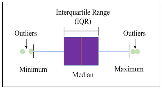
Figure 1.
The box plot method.
Based on the mechanism knowledge and correlation analysis, the characterization parameters with greater influence on gas kick risk were selected, and the smaller or irrelevant characterization parameters were removed, thus reducing the input dimension of the model. Pearson’s correlation coefficient is the ratio of the covariance of and variables to the product of the standard deviations of the two variables. So, the standard deviation of and cannot be zero. It reflects the direction and degree of the changing trend between the two variables. Its value ranges from −1.0 to +1. 0 means that the two variables are not correlated. A positive value means a positive correlation, a negative value means a negative correlation, and the larger the value, the stronger the correlation.
where is the correlation coefficient, is the covariance of and , is the standard deviation of , is the standard deviation of .
When explaining the degree of linear correlation between variables, according to experience, as is shown in Table 1, the degree of correlation can be divided into the following cases according to the size of the correlation coefficient:

Table 1.
Correlation coefficient.
By calculating and screening the highly correlated parameters and combining the mechanism knowledge, eight parameters were finally determined as input parameters: Outlet Rate, Instantaneous Rate of Penetration, Torque, Mud Tanks Volume, StandPipe Pressure, Inlet Density, Outlet Density, and Total Hydrocarbon.
The dimensions of many drilling parameters vary frequently, which will have an impact on the outcomes of data analysis. Data normalization processing is required to resolve the comparability of data features in order to remove dimensional effects between features. Consequently, we must normalize all input parameters before model training. The specific calculation formula is as follows,
where is the data sample, the normalized value of , and are the maximum and minimum values of the variable .
2.1.3. Data Augmentation
The ability of the intelligent model can be validated by using overlap sampling for data augmentation due to the limited quantity of gas kick risk sample data. Data augmentation techniques such as picture rotation, translation, pruning, and scaling in computer vision are not fully applicable to sequential drilling data. In this paper, the overlapping sampling technique was adopted to expand the samples [19]. The overlapping sampling technique is that when training samples are collected from the original signals of each drilling parameter, there is an overlap between each signal and the previous signal. The sampling method is shown in Figure 2. For drilling parameter signals, the offset is set as 1, and the overlap is set as 29; that is, the sampling window length is 30. The 8229 data points in the drilling parameter signals of the gas kick samples utilized in this paper, the sampling window length is 30, and the offset is 8200 gas kick samples can be made. There were only roughly 270 gas kick samples prior to the overlapping sampling approach.
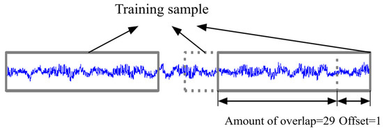
Figure 2.
Schematic diagram of overlap sampling.
2.2. Model Building
2.2.1. Long Short-Term Memory
Long Short-Term Memory (LSTM) is a special Recurrent Neural Network (RNN) proposed by Hochreiter and Schmidhuber in 1997. Optimized in 1999 by Alex Gloves et al. [20], this leads to a systematic and complete LSTM framework suitable for handling contextual dependencies between long sequences of data. It overcomes the disadvantages of disappearing RNN gradients (explosions) and the difficulty of retaining long-term memory. LSTM unit can be forgotten door (𝑓), input (𝑖), and output (𝑜) gating door make information selectively add or reduce, make it have long short-term memory ability. The LSTM structure is shown in Figure 3.
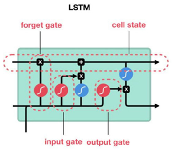
Figure 3.
LSTM network structure.
Each gate of LSTM controls the flow of information into, out of, and retention in the cell, enabling LSTM to effectively handle long sequential data and prevent gradient vanishing. LSTM also includes an internal state for storing and passing long-term memory information. Through the synergy of these gates and states, LSTM can learn long-term dependencies in the data and is widely used in natural language processing, speech recognition, and other fields.
2.2.2. Bidirectional Long Short-Term Memory
In the standard LSTM, the state transmission of each unit is one-way from the front to the back, and the output of the next moment can only be predicted based on the time sequence information of the previous moment. Therefore, the LSTM model can only learn the characteristics of the risk characterization parameters of the past moment but cannot learn the characteristics of the future moment. Bidirectional Long Short-Term Memory (BiLSTM) has two cell state belts that transmit information from the front to the front and from the back [21]. The bidirectional layer is composed of two opposite LSTM layers: the forward LSTM and the backward LSTM. Mining the relationship between the past and future data of temporal series, improving the data utilization rate, and making better use of the temporal characteristics of temporal series, to improve the accuracy of the model prediction.
BiLSTM network structure is shown in Figure 4. BiLSTM network is a bidirectional cyclic structure combining forward and reverse, which can better mine the correlation features of temporal series data.
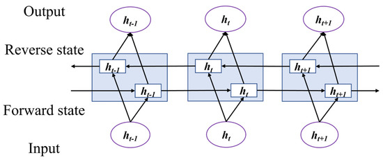
Figure 4.
BiLSTM network structure.
To postulate that for t positive LSTM hidden layer of network state, its computation formula, such as Equation (3), can be regarded as a single LSTM network. By − 1-moment state, calculate t moment state process, for t time input.
where, for t moment forward LSTM network hidden layer state; LSTM is the LSTM unit; for t moment input; as − 1 moment state forward LSTM network hidden layer state.
Similar to t moments reverse LSTM hidden layer of network state, the calculation formula is shown in Equation (4).
where for t moments reverse LSTM network hidden layer state; LSTM is the LSTM unit; for t moment input; for − 1 moment state back LSTM network hidden layer state. BiLSTM network output is two parts hidden layer state and combination together, thus forming the overall network hidden state.
2.2.3. Autoencoder
Autoencoder (AE) is a kind of artificial neural network which can be used for unsupervised learning [22]. It can automatically learn effective features from large amounts of unlabeled data. Autoencoders and their variants have been successfully applied in a wide range of fields, including data classification, anomaly detection, pattern recognition, data generation, product recommendation, etc. The autoencoder is mainly composed of an encoder and a decoder, and its structure is shown in Figure 5. The encoder and decoder of the temporal autoencoder model are both temporal networks. The encoder and decoder of the non-temporal autoencoder model are both non-temporal networks. For example, the encoder and decoder of the BiLSTM-AE model are BiLSTM, the encoder and decoder of the LSTM-AE model are LSTM, and the encoder and decoder of the MLP-AE model are MLP.
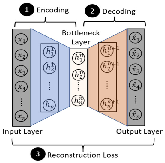
Figure 5.
Autoencoder structure [23].
The encoder and decoder can be defined as the function ϕ: and ψ: . The goal of the autoencoder is to fit an identity function, as shown in Equation (5):
In the encoding phase, the autoencoder maps the input vector to the intermediate vector using the function shown in Equation (6), and m > n.
where is a weight matrix, is a bias vector, and is the activation function of the encoding layer.
In the decoding stage, the autoencoder maps the intermediate vector to the output vector through Equation (7), and m > n. Then, use Equation (8) to calculate the refactoring vector and the input vector of the original the reconstruction error between the two.
where is the weight matrix, is an offset vector, is a coding layer activation function.
On this basis, the goal of the autoencoder is to minimize the reconstruction error. This is equivalent to spread by gradient descent and reverse to learn proper weight matrix and and offset vector and minimize the .
2.2.4. MLP-AE
The multilayer perceptron (MLP) consists of an input layer, multiple hidden layers and an output layer; each layer is connected by multiple neuron nodes [24]. The MLP-AE model has a straightforward structure that makes it simple to comprehend and use. It is made up of a decoder and an encoder. The input drilling data is compressed by the encoder into a low-dimensional code, which is then uncompressed by the decoder to produce reconstructed data. The MLP is initially used to process the raw drill data, and the fully connected layers are then subjected to a series of nonlinear modifications to produce low-dimensional coding. After giving the decoder the code, we obtain the reconstructed data by putting a full connection layer through a sequence of nonlinear operations in reverse. Finally, we use the trained MLP-AE model to analyze and forecast drilling data. By comparing the discrepancies between the predicted and actual drilling data, we further investigate the features and rules of drilling data.
2.2.5. BiLSTM-AE
As seen in Figure 6, the BiLSTM-AE model uses the BiLSTM network for both the encoder and decoder. The model’s input and output are sequences. The BiLSTM-AE model is trained to recognize sequential patterns in normal time series [25,26]. When the temporal series is input into the depth encoder, the model can quickly recognize and preserve the sequence patterns in the majority of normal series, and its reconstruction error is fairly low. On the other hand, for a few risk series for which the model finds it difficult to extract their sequence patterns, the reconstruction error is comparatively substantial. By computing the reconstruction error between the reconstructed sequence and the original series and establishing the threshold value in accordance with the mechanical knowledge and data characteristics, the series with a reconstruction error greater than the threshold value is recognized as the risk series.
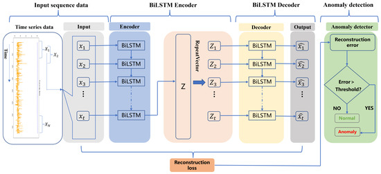
Figure 6.
Structure of the BiLSTM-AE model [23].
2.3. Threshold Setting
If the data reconstruction error exceeds the predetermined threshold, the unsupervised autoencoder model classifies the data as abnormal. The threshold for this paper is set at 1.0 and can be altered depending on the data’s features and the field’s needs. This threshold is decided by an understanding of the mechanism and its properties.
Additionally, the temporal autoencoder’s abnormal sequence is fitted using the least square method to see if it follows the trend of gas kick risk. Finally, to further confirm the gas kick risk, we fixed the time series’ slope at 0.0018 based on the experience of the industry. Once more, this threshold can be changed as necessary.
2.4. Evaluation Metrics
From a certain point of view, anomaly detection can be regarded as a classification problem. Samples can be divided into true positive (TP), true negative (TN), false positive (FP), and false negative (FN), and thus the confusion matrix is shown in Table 2.

Table 2.
Confusion matrix.
Based on the confusion matrix in Table 2, four important evaluation indexes of anomaly detection methods can be calculated, namely , , , and , which can be calculated by the following formula:
: The proportion of all correct predictions in the total sample.
: The proportion of predicted positive samples to the actual positive samples.
: The proportion of true positive samples among all the samples predicted as positive by the model.
: Harmonic mean of and .
- : True Positive, Positive samples are classified as positive samples;
- : False Positive, Negative samples are classified as positive samples;
- : True Negative, Negative samples are classified as negative samples;
- : False Negative, Positive samples are classified as negative samples.
3. Results and Discussion
3.1. Optimal Sequence Length
When utilizing a model of temporal intelligence, the optimization of temporal series length is crucial. The model’s ability to predict outcomes accurately can be increased by selecting the right length of temporal series. A temporal series that is too long or too short can produce incorrect predictions. The risk of overfitting or underfitting can be decreased with the right time series length. The model may overfit the past data if the temporal series is too long, which will result in erroneous predictions for the incoming data. The model might not be able to acquire enough patterns if the temporal series is too long and too short, which would lead to underfitting. The experimental results are shown in Figure 7.
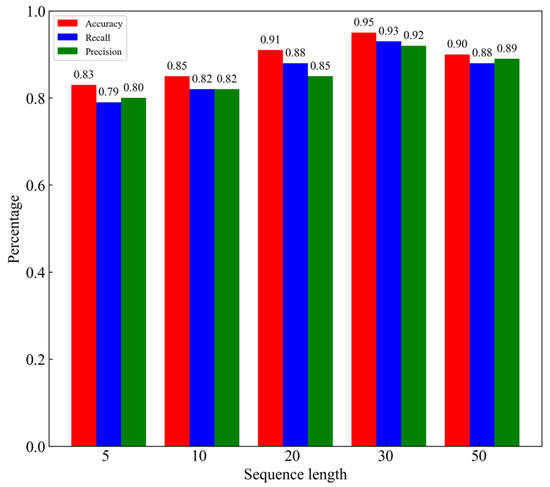
Figure 7.
Experimental results for different sequence lengths.
The greatest accuracy value is 0.95 when the sequence length is 30. This indicates that the model’s overall prediction accuracy is highest for temporal series lengths of 30. When the temporal series length was 30, the maximum values for recall and precision were 0.93 and 0.92, respectively. This indicates that the model operates most effectively with temporal series of length 30.
3.2. Model Parameter
In this study, we use TensorFlow to build the LSTM model, the MLP-AE model, the LSTM-AE model and the BiLSTM-AE model for gas kick risk temporal series detection. The last three models are unsupervised, while only the LSTM model is supervised. All network parameters are set uniformly in order to make the models comparable and maintain a consistent level of model complexity. The input to the MLP-AE model is a one-dimensional vector containing 240 unique variables. The 30 × 8 matrix serving as the input for the LSTM, LSTM-AE, and BiLSTM-AE models has eight characteristics per time step and represents a 30-period window. The structure parameters of each network model are shown in Table 3.

Table 3.
Parameters of LSTM, MLP-AE, LSTM-AE, BiLSTM-AE model.
3.3. Model Comparison
In this section, we compare and analyze the performance of gas kick intelligent warning models, find out the advantages of different models to capture features, and finally select and evaluate the best intelligent prediction model. The experimental evaluation results are shown in Table 4.

Table 4.
Experimental evaluation results.
The sequential model performs better than the non-sequential model, while the MLP-AE model has the worst effect, as can be seen from the model comparison in Table 4. It is possible to recognize and foresee patterns and changes in risk data by taking data timeliness into account. Additionally, the unsupervised sequential autoencoder model performs better than the traditional sequential model.
It can be seen from the results that the accuracy of the LSTM-AE model is increased by 6% compared with the LSTM model, and the recall rate and accuracy rate are increased by 7% and 4%, respectively. Therefore, the biLSTM-AE model has the best effect; its accuracy is increased by 10% compared with LSTM, its accuracy is increased by 4% compared with LSTM-AE, and its recall rate and accuracy rate are increased by 4% and 3% compared with LSTM-AE model. In addition, it can be seen from Figure 8 and Figure 9 that the LSTM-AE model has the gas kick risk underreporting, while BiLSTM-AE does not. This is because BiLSTM may take into account both past and future information at the same time through forward and reverse propagation, which allows for the collection of more thorough contextual data and an increase in model accuracy.
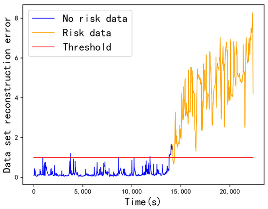
Figure 8.
LSTM-AE model results.
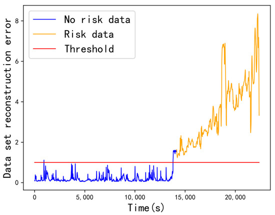
Figure 9.
BiLSTM-AE model results.
Input series encoding and reconstruction using BiLSTM network as autoencoder. BiLSTM can handle long-term dependencies in drilling temporal series data because the gated units in the BiLSTM network structure can adaptively control the flow of information and selectively forget or remember information from it; BiLSTM is robust and can handle series of any length.
The LSTM-AE and BiLSTM-AE models are unsupervised, and drilling site gas kick risk data are not labeled, so the application of unsupervised models is significant. It can be seen from the results that the effect of the unsupervised model is better than that of a supervised model. BiLSTM can take into account both forward and reverse information of the input series and utilize two-way information processing to extract sequence features better. Therefore, BiLSTM has a better risk detection effect than LSTM.
The Mud Tanks Volume sequence is displayed in Figure 10 as an example. As can be seen, the slope of the abnormal sequence is definitely larger than that of the normal sequence data, showing that the Mud Tanks Volume shows an increasing trend and further confirming that the risk is the gas kick.
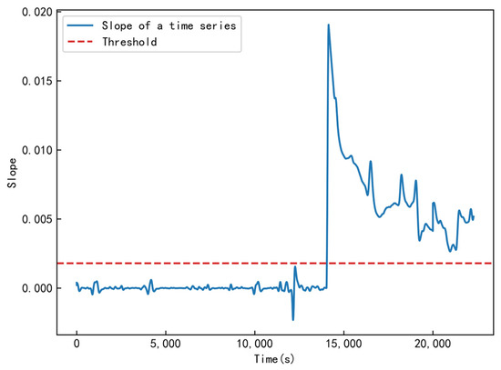
Figure 10.
The slope of the sequence data.
4. Conclusions
A new method for the gas kick risk warning is proposed, which is based on an unsupervised temporal autoencoder model and is of great significance for the future development of the gas kick risk warning. In practical applications, the driller monitors the signal equipment. If the output reconstruction error of the signal input to the model is greater than the set threshold, and the changing trend is consistent with the risk characteristics, the risk of gas kick is determined.
While the temporal model can extract the temporal features of the evolution of drilling risk, the MLP-AE model is unable to extract the contextual features of the temporal series of the data. As a result, the temporal model performs better than the non-temporal MLP-AE model.
In this study, the performance of the unsupervised temporal autoencoder model is better than that of the supervised model. BiLSTM-AE model has the best effect, and its accuracy rate is increased by 10% compared with LSTM, 4% compared with LSTM-AE, recall rate, and accuracy rate are increased by 4% and 3% compared with LSTM-AE model, and there is no risk underreporting. This approach has a prospective application because risk data from drilling sites are not labeled.
The temporal autoencoder for the gas kick risk warning can be further investigated in this research in order to create a more reliable model. Future research will focus on the model’s interpretability in an effort to develop a superior intelligent model for the gas kick risk warning.
Author Contributions
Conceptualization, Z.Z. and X.S.; methodology, Z.Z.; software, D.Z.; validation, Z.Z. and D.Z.; formal analysis, Z.Z.; investigation, Z.Z.; resources, X.S.; data curation, D.Z.; writing—original draft preparation, D.Z.; writing—review and editing, Z.Z., D.Y., M.Z., C.Z. and S.D.; visualization, D.Z. and L.Z.; supervision, Z.Z.; project administration, Z.Z.; funding acquisition, X.S. and M.Z. All authors have read and agreed to the published version of the manuscript.
Funding
This research was funded by National Key Research and Development Project, grant number 2019YFA07083004, National Science Foundation for Distinguished Young Scholars, grant number 52125401, Science Foundation of China University of Petroleum, Beijing (No.2462022QNXZ004), the National Natural Science Foundation of China (Grant No. 52274019), Science Foundation of China University of Petroleum, Beijing, grant number 2462022SZBH002.
Data Availability Statement
The data are not publicly available due to involve the information on Chinese oil fields and need to be kept confidential.
Acknowledgments
The author would like to thank the High-Pressure Water Jet Drilling and Completion Laboratory of China University of Petroleum, Beijing.
Conflicts of Interest
The authors declare no conflict of interest.
References
- Menghan, S. Study on Real-Time Warning Method of Drilling Overflow; Southwest Petroleum University: Chengdu, China, 2016. [Google Scholar]
- Du, Z. Research on Intelligent Identification and Diagnosis of Overflow; China University of Petroleum: Beijing, China, 2020. [Google Scholar]
- Shoujun, L. Development of device for drilling fluid level detection and automatic grout system. China Pet. Mach. 2006, 34, 29–30. [Google Scholar]
- Jiang, Q.; Wang, Y.; Mao, M.; Wang, Y.; Li, Z. Early kick detection system based on Coriolis mass flowmeter. J. Oil Gas Technol. 2013, 35, 158–160. [Google Scholar]
- Hou Yan-Wei, L.X. Application effect and development direction of engineering logging early warning system in drilling site. Pet. Instrum. 2013, 27, 6–9. [Google Scholar]
- Jinbo, W.; Baojiang, S.; Hao, L.I.; Ning, W.; Zhiyuan, W.; Yonghai, G. Early gas kick detection based on the LWD resistivity in deepwater drilling. J. China Univ. Pet. (Ed. Nat. Sci.) 2017, 41, 94–100. [Google Scholar]
- Ying, Z. Research on Data-Driven Early Warning and Treatment Methods for Deepwater Gas Kick; China University of Petroleum: Beijing, China, 2020. [Google Scholar]
- Kamyab, M.; Shadizadeh, S.R.; Jazayeri-rad, H.; Dinarvand, N. In Early kick detection using real time data analysis with dynamic neural network: A case study in iranian oil fields. In Proceedings of the Nigeria Annual International Conference and Exhibition, Calabar, Nigeria, 7 July 2010; OnePetro: Richardson, TX, USA, 2010. [Google Scholar]
- Gola, G.; Nybø, R.; Sui, D.; Roverso, D. In Improving management and control of drilling operations with artificial intelligence. In Proceedings of the SPE Intelligent Energy International, Utrecht, The Netherlands, 27–29 March 2012; OnePetro: Richardson, TX, USA, 2012. [Google Scholar]
- Weijie, Y. Design and Development of on-Line Monitoring and Early Warning System for “Three High” Oil and Gas Well Overflow Aura; China University of Petroleum (East China): Beijing, China, 2014. [Google Scholar]
- Luzhi, Z.; Haibo, L.; Jin, Z.; Ling, M. Application of BP neural network in the intelligent early warning of drilling overflow in development Wells. Inf. Commun. 2014, 2, 3–4. [Google Scholar]
- Liang, H.; Li, G.; Liang, W. Intelligent early warning model of early-stage overflow based on dynamic clustering. Clust. Comput. 2019, 22, 481–492. [Google Scholar] [CrossRef]
- Yin, Q.; Yang, J.; Tyagi, M.; Zhou, X.; Wang, N.; Tong, G.; Xie, R.; Liu, H.; Cao, B. Downhole quantitative evaluation of gas kick during deepwater drilling with deep learning using pilot-scale rig data. J. Petrol. Sci. Eng. 2022, 208, 109136. [Google Scholar] [CrossRef]
- Li, H.; Ge, Z.; Wei, N.; Sun, W.; Zhang, Y.; Xue, J.; Jiang, L.; Pei, J.; Liao, B.; Cao, H. Research on intelligent judgment method of natural gas hydrate drilling risk. Petroleum 2021, 7, 439–450. [Google Scholar] [CrossRef]
- Jiang, H.; Liu, G.; Li, J.; Zhang, T.; Wang, C. A realtime drilling risks monitoring method integrating wellbore hydraulics model and streaming-data-driven model parameter inversion algorithm. J. Nat. Gas Sci. Eng. 2021, 85, 103702. [Google Scholar] [CrossRef]
- Elmgerbi, A.; Thonhauser, G. Holistic autonomous model for early detection of downhole drilling problems in real-time. Process Saf Env. 2022, 164, 418–434. [Google Scholar] [CrossRef]
- Wanjun, H.; Wenhe, X.; Yongjie, L.; JIANG, J.; Gao, L.I.; Yijian, C. An intelligent identification method of safety risk while drilling in gas drilling. Petrol. Explor Dev. 2022, 49, 428–437. [Google Scholar]
- Tukey, J.W. Exploratory Data Analysis; Addison-Wesley: Reading, MA, USA, 1977; Volume 2. [Google Scholar]
- Wei, Z. Study on Bearing Fault Diagnosis Algorithm Based on Convolutional Neural Network. Master’s Thesis, Harbin Institute of Technology, Harbin, China, 2017. [Google Scholar]
- Gers, F.A.; Schmidhuber, J.; Cummins, F. Learning to forget: Continual prediction with LSTM. Neural Comput. 2000, 12, 2451–2471. [Google Scholar] [CrossRef] [PubMed]
- Schuster, M.; Paliwal, K.K. Bidirectional recurrent neural networks. IEEE T Signal Proces. 1997, 45, 2673–2681. [Google Scholar] [CrossRef]
- An, J.; Cho, S. Variational autoencoder based anomaly detection using reconstruction probability. Spec. Lect. IE 2015, 2, 1–18. [Google Scholar]
- Wei, Y.; Jang-Jaccard, J.; Xu, W.; Sabrina, F.; Camtepe, S.; Boulic, M. Lstm-autoencoder based anomaly detection for indoor air quality time series data. IEEE Sens J. 2023, 23, 3787–3800. [Google Scholar] [CrossRef]
- Pinkus, A. Approximation theory of the MLP model in neural networks. Acta Numer. 1999, 8, 143–195. [Google Scholar] [CrossRef]
- Serai, P.; Stiff, A.; Fosler-Lussier, E. In End to end speech recognition error prediction with sequence to sequence learning. In Proceedings of the ICASSP 2020–2020 IEEE International Conference on Acoustics, Speech and Signal Processing (ICASSP), Barcelona, Spain, 4–8 May 2020; IEEE: New York, NY, USA, 2020; pp. 6339–6343. [Google Scholar]
- Meneghello, F.; Rossi, M.; Bui, N. Smartphone identification via passive traffic fingerprinting: A sequence-to-sequence learning approach. IEEE Netw. 2020, 34, 112–120. [Google Scholar] [CrossRef]
Disclaimer/Publisher’s Note: The statements, opinions and data contained in all publications are solely those of the individual author(s) and contributor(s) and not of MDPI and/or the editor(s). MDPI and/or the editor(s) disclaim responsibility for any injury to people or property resulting from any ideas, methods, instructions or products referred to in the content. |
© 2023 by the authors. Licensee MDPI, Basel, Switzerland. This article is an open access article distributed under the terms and conditions of the Creative Commons Attribution (CC BY) license (https://creativecommons.org/licenses/by/4.0/).